Dynamics of charge-displacement channeling in intense laser-plasma interactions
Abstract
The dynamics of transient electric fields generated by the interaction of high intensity laser pulses with underdense plasmas has been studied experimentally with the proton projection imaging technique. The formation of a charged channel, the propagation of its front edge and the late electric field evolution have been characterised with high temporal and spatial resolution. Particle-in-cell simulations and an electrostatic, ponderomotive model reproduce the experimental features and trace them back to the ponderomotive expulsion of electrons and the subsequent ion acceleration.
pacs:
52.27.Ny, 52.38.-r, 52.38.Hb, 52.38.Kd1 Introduction
The study of the propagation of intense laser pulses in underdense plasmas is relevant to several highly advanced applications, including electron [1] and ion acceleration [2, 3], development of X- and -ray sources [4], and fusion neutron production [5]. It is also of fundamental interest, due to the variety of relativistic and nonlinear phenomena which arise in the laser-plasma interaction [6]. Among these, self-focusing and self-channeling of the laser pulse arise in this regime from the intensity dependence of the relativistic index of refraction [7, 8].
Strong space charge electric fields are generated during the early stage of the propagation of a superintense laser pulse through an underdense plasma as the ponderomotive force acts on electrons, pushing them away from the axis. Thus, for a transient stage the pulse may propagate self-guided in a charged channel [9], while the space-charge field in turn drags and accelerates the ions to MeV energies[3]. So far, experiments have provided evidence of channel formation and explosion using optical diagnostics [9, 10, 11, 12, 13, 14]. or by detecting radially accelerated ions [2, 3, 5, 14], while a direct detection of the space-charge fields has not been obtained yet. The development of the the proton projection imaging (PPI) technique [15] has provided a very powerful tool to explore the fast dynamics of plasma phenomena via the detection of the associated transient electric field structures. The technique is based on the use of laser-accelerated multi-MeV protons ([16, 17] and references therein) as a charged probe beam of transient electromagnetic fields in plasmas, a possibility allowed by the low emittance and high laminarity of the proton source [18, 19], as well as by its ultra-short duration and the straightforward synchronization with an interaction laser pulse. The experimental PPI implementation takes advantage from the broad energy spectrum of protons, since in a time-of-flight arrangement protons of different energy will probe the plasma at different times, and thus an energy-resolved monitoring of the proton probe profile allows to obtain single-shot, multi-frame temporal scans of the interaction [15]. PPI and the related ”proton deflectometry” technique permit to gather spatial and temporal maps of the electric fields in the plasma, and therefore have proven to be an unique tool to explore the picosecond dynamics of laser-plasma phenomena [20, 21, 22] via the associated space-charge fields.
In this article, we report on an experiment using the PPI technique to study of the formation and subsequent evolution of a charge-displacement channel in an underdense plasma. These investigations have led to the first direct experimental detection of the transient electric fields in the channel, providing an insight of the fundamental physical processes involved. The comparison of the experimental data with two-dimensional (2D) electromagnetic (EM) particle-in-cell (PIC) simulations and a simple one-dimensional (1D) electrostatic (ES) PIC model allows to characterize in detail the electric field dynamics at different stages of its evolution.
2 Experimental setup
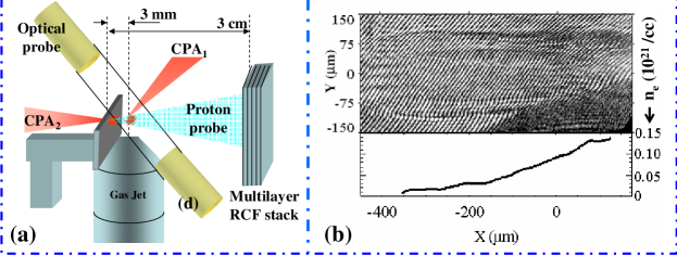
The experiment was carried out at the Rutherford Appleton Laboratory, employing the VULCAN Nd-Glass laser system [23], providing two Chirped Pulse Amplified (CPA) pulses, with wavelength, synchronized with picosecond precision. Each of the beams delivered approximately 30 J on target in 1.3 ps (FWHM) duration. By using off-axis parabolas, the beams were focused to spots of (FWHM) achieving peak intensities up to . The short pulses were preceded by an Amplified Spontaneous Emission (ASE) pedestal of 300 ps duration and contrast ratio of [24]. One of the beams () was directed to propagate through He gas from a supersonic nozzle, having a 2 mm aperture, driven at 50 bar pressure. The interaction was transversely probed by the proton beam produced from the interaction of the second CPA beam () with a flat foil (a thick Au foil was typically used), under the point projection imaging scheme [15]. The schematic of the experimental setup is shown in Fig.1(a). Due to the Bragg peak energy deposition properties of the protons, the use of multilayered stacks of Radiochromic film (RCF) detector permits energy-resolved monitoring of the proton probe profile, as each layer will primarily detect protons within a given energy range. This allows to obtain single-shot, multi-frame temporal scans of the interaction in a time-of-flight arrangement [15]. The spatial and temporal resolution of each frame were of the order of a few ps, and of a few microns, respectively, while the magnification was 11.
The interaction region was also diagnosed by Nomarsky interferometry, employing a frequency doubled CPA pulse of low energy. The reconstructed electron density profile along the propagation axis before the high-intensity interaction [see Fig. 1(b)], broadly consistent with the neutral density profile of the gas jet [25] suggests complete ionisation of the gas by the ASE prepulse.
3 Experimental Results
Fig. 2(a), (b) and (c) show three sequential proton-projection images of the interaction region. The laser pulse propagates from left to right. A ’white’ channel with ’dark’ boundaries is visible at early times [Fig.2 (a) and (b)]. The leading, ’bullet’ shaped edge of the channel, indicated by the label I in Fig.2 (a) and (b), is seen moving along the laser axis. In the trail of the channel the proton flux distribution changes qualitatively [Fig. 2(c) and (d)], showing a dark line along the axis (indicated by the label III), which is observed up to tens of ps after the transit of the peak of the pulse. The ’white’ channel reveals the presence of a positively charged region around the laser axis, where the electric field points outwards.
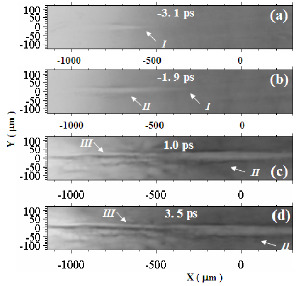
This can be interpreted as the result of the expulsion of electrons from the central region. The central dark line observed at later times in the channel suggests that at this stage the radial electric field must change its sign, i.e. point inwards, at some radial position. As discussed below, this field inversion is related to the effects of ion motion.
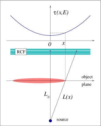
Due to multi-frame capability of the PPI technique with ps temporal resolution, it has been possible to estimate the propagation velocity of the channel front. Critically, one has to take into account that, due to the divergence of the probe beam, the probing time varies along the pulse propagation axis (see Fig. 3) as where is the distance between the plane and the proton source and is the proton time of flight from the source to the center of the object plane (see Fig.3). The reference time is relative to the instant at which the laser pulse peak crosses the focal plane . We divide the displacement of the tip of the channel leading front from frame (a) to (b), by the difference in the corresponding probing times to obtain . Based on the nominal reference time we estimate the peak of the pulse to be approximately behind the tip of the channel front.
4 Data analysis by numerical simulations
In order to unfold the physical mechanisms associated with the dynamics of the charged channel, a 1D ES PIC model in cylindrical geometry was employed, in which the laser action is modeled solely via the ponderomotive force (PF) of a non-evolving laser pulse. A similar approach has been previously used by other authors [12, 14]. The code solves the equation of motion for plasma particles along the radial direction, taking into account the ES field obtained from Poisson’s equation and the PF acting on the electrons - [26]. Here and defines the temporal envelope of the laser pulse. For the latter, a ’’ profile was used (the use of a Gaussian profile did not yield significant differences).

Fig. 4 shows the electric field and the ion density obtained from a simulation with , and initial density . The initial depletion of electrons and the later formation of an ambipolar electric field front are clearly evident. In order to achieve a direct comparison with the experimental data, a 3D particle tracing simulation, employing the PTRACE code [22], was carried out to obtain the proton images for an electric field given by . The experimental proton source characteristics (e.g. spectrum and divergence), the detector configuration and dose response were taken into account. A simulated proton image, reproducing well the main features observed in the experiment, is shown in Fig. 4(c). The tip of the channel front is located ahead of the pulse peak, in fair agreement with the previous estimate based on the data.
An essential description theoretical description of the dynamics observed in the 1D simulations can be given as follows (a detailed description is reported in Ref.[27]). In the first stage, pushes part of the electrons outwards, quickly creating a positively charged channel along the axis and a radial ES field which holds the electrons back, balancing almost exactly the PF, i.e. ; thus, the electrons are in a quasi–equilibrium state, and no significant electron heating occurs. Meanwhile, the force accelerates the ions producing a depression in around the axis [see Fig.4 (b)]; at the end of the pulse () we find [see Fig.4 (a)], indicating that the ions have reached the electrons and restored the local charge neutrality. However, the ions retain the velocity acquired during the acceleration stage. For , where is the position of the PF maximum, the force on the ions, and thus the ion final velocity, decrease with ; as a consequence, the ions starting at a position are ballistically focused towards a narrow region at the edge of the intensity profile, and reach approximately the same position () at the same time (, i.e. after the peak of the laser pulse); here they pile up producing a very sharp peak of . Correspondingly, the ion phase space shows that the fastest ions (with energies , of the order of the time-averaged ponderomotive potential) overturn the slowest ones and hydrodynamical breaking of the ion fluid occurs. Using a simple model [27], the “breaking” time and position can be estimated to be (where is the time at which the pulse has maximum amplitude) and , yielding and for the simulation in Fig.4, in good agreement with the numerical results. As inferred from the ion phase space plot at , a few ions acquire negative velocity after “breaking”; they return toward the axis and lead to the formation of a local density maximum at after .
The electron phase space shows that at breaking the electrons are strongly heated around the ion density peak, generating an “hot” electron population with a “temperature” and a density , corresponding to a local Debye length is . A modeling of the sheath field thus generated around the density spike [27] (whose thickness is less than both and the sheath width ) yields a peak field and a sheath width , consistently with the simulation results. The ambipolar field at the “breaking” location can be thus be interpreted as the sheath field resulting from the local electron heating.
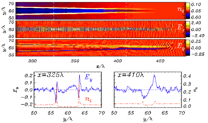
The good agreement of the simulated image with the experimental ones indicates that the 1D ponderomotive, electrostatic model contains the essential physics of self-channeling and related electric field dynamics, despite the exclusion of nonlinear pulse evolution due, e.g., to self-focusing, or of the plasma inhomogeneity. To address these issues we performed electromagnetic particle-in-cell simulations of the laser-plasma interaction. The simulation were two-dimensional (2D) in planar geometry - a fully 3D simulation with spatial and temporal scales close to the experimental ones and adequate numerical resolutions is way beyond present days computational power. The 2D results can be considered to be qualitative since, for instance, the diffraction length of the laser beam or the scaling with distance of the electrostatic field are different in 3D. Despite of these limitations, the main features of the channel observed in the experimental data are qualitatively reproduced in 2D simulations for a range of parameters close to the experiment. In the simulation of Fig. 5, the laser pulse has a Gaussian intensity profile both in space and time, with peak dimensionless amplitude , radius and duration where is the laser wavelength. For the pulse duration and intensity correspond to and , respectively. The charge-to-mass ratio of ions is . The electron density grows linearly along the -axis from zero to the peak value (where is the critical density and for ) over a length of , and then remains uniform for . A numerical grid, a spatial resolution and particles per cell for both electrons and ions were used.
Fig. 5 shows the ion density () and the components and of the electric field at the time . In this simulation the laser pulse is -polarized, i.e. the polarization is along the axis, perpendicular to the simulation plane. Thus, in Fig. 5 is representative of the amplitude of the propagating EM pulse, while is generated by the space-charge displacement. Simulations performed for the case of -polarization showed no substantial differences in the electrostatic field pattern. The simulation clearly shows the formation of an electron-depleted channel, resulting in an outwardly directed radial space-charge electric field whose peak value is (see the lineout at in Fig.5). In the region behind the peak of the pulse, two narrow ambipolar fronts (one on either side of the propagation axis) are observed. The ambipolar fields have peak values of (see the lineout at in Fig.5). As shown above, such a radial electric field profile produces a pattern in the proton images similar to that observed in region (III) of Fig. 2.
5 Conclusion
We have reported the first direct experimental study of the electric field dynamics in a charge-displacement channel produced by the interaction of a high intensity laser pulse with an underdense plasma. The field profiles observed clearly identify different stages of the channel evolution: the electron depletion near the axis due to the ponderomotive force, and the following ion acceleration causing a field inversion along the radius. The features observed are reproduced and interpreted by means of 1D electrostatic and 2D electromagnetic PIC simulations, followed by a reconstruction of the proton images employing a 3D particle tracing code.
Acknowledgements
This work has been supported by an EPSRC grant, Royal Society Joint Project and Short Visit Grants, British-Council-MURST-CRUI, TR18 and GRK1203 networks, and MIUR (Italy) via a PRIN project. Part of the simulations were performed at CINECA (Bologna, Italy) sponsored by the INFM super-computing initiative. We acknowledge useful discussions with F. Cornolti and F. Pegoraro and the support of J. Fuchs and the staffs at the Central Laser Facility, RAL (UK).
References
References
- [1] Malka V. et al., Plasma Phys. Control. Fusion, 47, B481 (2005) and the references therein.
- [2] Krushelnick K. et al., Phys. Rev. Lett., 83, 737 (1999); Wei M. S. et al., ibid. 93, 155003 (2004).
- [3] Willingale L. et al., Phys. Rev. Lett., 96, 245002 (2006).
- [4] Rousse A. et al., Phys. Rev. Lett., 93, 135005 (2004).
- [5] Fritzler S. et al., Phys. Rev. Lett., 89, 165004 (2002).
- [6] Bulanov S. V. et al., Rev. Plasma Phys., 22, 227 (2001).
- [7] Sun G. Z. et al., Phys. Fluids, 30, 526 (1987).
- [8] Mori W. B. et al., Phys. Rev. Lett., 60, 1298 (1988).
- [9] Borisov A. B. et al., Phys. Rev. Lett., 68, 2309 (1992); Borisov A. B. et al., Phys. Rev.A 45, 5830 (1992).
- [10] Monot P. et al., Phys. Rev. Lett., 74, 2953 (1995).
- [11] Borghesi M. et al., Phys. Rev. Lett., 78, 879 (1997).
- [12] Krushelnick K. et al., Phys. Rev. Lett., 78, 4047 (1997).
- [13] Sarkisov G.S. et al., JETP Lett., 66, 828 (1997).
- [14] Sarkisov G. S. et al., Phys. Rev.E, 59, 7042 (1999).
- [15] Borghesi M. et al., Rev. Sci. Instrum., 74, 1688 (2003).
- [16] Fuchs J. et al., Nature Phys., 2, 48-54 (2006).
- [17] Robson L. et. al., Nature Phys., 3, 58 (2006).
- [18] Borghesi M. et al., Phys. Rev. Lett., 92, 055003 (2006).
- [19] Cowan T. et al., Phys. Rev. Lett., 92, 204801 (2006).
- [20] Borghesi M. et al., Phys. Rev. Lett., 88, 135002 (2002).
- [21] Borghesi M. et al., Phys. Rev. Lett., 94, 195003 (2005).
- [22] Romagnani L. et al., Phys. Rev. Lett., 95, 195001 (2005).
- [23] Danson C. et al., J.Mod.Opt., 45, 1653 (1998).
- [24] Gregori G., Central Laser Facility, RAL, UK, private communication.
- [25] Jung R. et al., in: Central Laser Facility Annual Report 2004/2005, RAL Report No. RAL-TR-2005-025, p.23.
- [26] Bauer D., Mulser P. and Steeb W. H., Phys. Rev. Lett., 94, 195003 (2005).
- [27] Macchi A. et al., physics/0701139.