Module identification in bipartite and directed networks

Abstract

Modularity is one of the most prominent properties of real-world complex networks. Here, we address the issue of module identification in two important classes of networks: bipartite networks and directed unipartite networks. Nodes in bipartite networks are divided into two non-overlapping sets, and the links must have one end node from each set. Directed unipartite networks only have one type of nodes, but links have an origin and an end. We show that directed unipartite networks can be conviniently represented as bipartite networks for module identification purposes. We report a novel approach especially suited for module detection in bipartite networks, and define a set of random networks that enable us to validate the new approach.

Units in physical, chemical, biological, technological, and social systems interact with each other defining complex networks that are neither fully regular nor fully random Albert and Barabási (2002); Newman (2003); Amaral and Ottino (2004). Among the most prominent and ubiquitous properties of these networks is their modular structure Girvan and Newman (2002); Newman (2003), that is, the existence of distinct groups of nodes with an excess of connections to each other and fewer connections to other nodes in the network.

The existence of modular structure is important in several regards. First, modules critically affect the dynamic behavior of the system. The modular structure of the air transportation system Guimerà et al. (2005a), for example, is likely to slow down the spread of viruses at an international scale Colizza et al. (2006a) and thus somewhat minimize the effects of high-connectivity nodes that may otherwise function as “super- spreaders” Pastor-Satorras and Vespignani (2001); Liljeros et al. (2003). Second, different modules in a complex modular network can have different structural properties Guimerà et al. (2007). Therefore, characterizing the network using only global average properties may result in the misrepresentation of the structure of many, if not all, of the modules. Finally, the modular structure of networks is likely responsible for at least some of the correlations (e.g. degree-degree correlations Newman (2002); Pastor-Satorras et al. (2001); Maslov and Sneppen (2002); Maslov et al. (2004); Colizza et al. (2006b)), that have attracted the interest of researchers in recent years Guimerà et al. (2007).

For the above reasons, considerable attention has been given to the development of algorithms and theoretical frameworks to identify and quantify the modular structure of networks (see Danon et al. (2005) and references therein). However, current research activity has paid little attention, except for a few studies in sociology Borgatti and Everett (1997); Doreian et al. (2004), to the problem of identifying modules in a special and important class of networks known as bipartite networks (or graphs). Nodes in bipartite networks are divided into two non-overlapping sets, and the links must have one end node from each set. Examples of systems that are more suitably represented as bipartite networks include:

• Protein-protein interaction networks Uetz et al. (2000); Jeong et al. (2001); Maslov and Sneppen (2002); Li et al. (2004) obtained from yeast two hybrid screening: one set of nodes represents the bait proteins and the other set represents the prey or library proteins. Two proteins, a bait and a library protein, are connected if the library protein binds to the bait.

• Plant-animal mutualistic networks Jordano (1987); Bascompte et al. (2003): one set represents animal species and the other set represents plant species. Links indicate mutualistic relationships between animals and plants (for example, a certain bird species feeding on a plant species and dispersing its seeds).

• Scientific publication networks Newman (2001); Börner et al. (2004); Guimerà et al. (2005b): one set represents scientists and the other set represents publications. A link between a scientist and a publication indicates that the scientist is one of the authors of the publication.

• Artistic collaboration networks Gleiser and Danon (2003); Uzzi and Spiro (2005); Guimerà et al. (2005b): one set represents artists and the other teams. A link indicates the participation of an artist in a team.

Another important class of networks for which no sound module identification methods are available are unipartite directed networks. Examples of directed unipartite networks include:

• Food webs Williams and Martinez (2000); Stouffer et al. (2005): nodes represent species and links indicate trophic interactions in an ecosystem.

• Gene regulatory networks Barabási and Oltvai (2004): nodes are genes and links indicate regulatory interactions.

The usual approach to identify modules in directed networks is to disregard the directionality of the connections, which will fail when different modules are defined based on incoming and outgoing links.

Here, we address the issue of module identification in complex bipartite networks. We start by reviewing the approaches that are currently used heuristically and aprioristically to solve this problem. We then suggest a new approach especially suited for module detection in bipartite networks, and define a set of random networks that permit the evaluation of the accuracy of the different approaches. We then discuss how it is possible to use the same formalism to identify modules in directed unipartite networks. Our method enables one to independently identify groups of nodes with similar outgoing connections and groups of nodes with similar incoming connections.

I Background

For simplicity, from now on we denote the two sets of nodes in the bipartite network as the set of actors and the set of teams, respectively. Given a bipartite network, we are interested in identifying groups (modules) of actors that are closely connected to each other through co-participation in many teams. Of course, one is free to select which set of nodes in a given network is the “actor set” and which one is the “team set,” so one can identify modules in either or both set of nodes.

We require any module-identification algorithm to fulfill two quite general conditions: (i) the algorithm needs to be network independent; and (ii) given the list of links in the network, the algorithm must determine not only a good partition of the nodes into modules, but also the number of modules and their sizes.

The first condition is somewhat trivial. We just make it explicit to exclude algorithms that are designed to work with a particular network or family of networks, but that will otherwise fail with broad families of networks (for example, large networks or sparse/dense networks).

The second condition is much more substantial, as it makes clear the difference between the module-identification problem and the graph partitioning problem in computer science, in which both the number of groups and the sizes of the groups are fixed. To use a unipartite network analogy, given a set of 120 people attending a wedding and information about who knows whom, the graph partitioning problem is analogous to optimally setting 12 tables with 10 people in each table. In contrast, the module-identification problem is analogous to identifying “natural” groups of people, for example the different families or distinct groups of friends.

The second condition also excludes algorithms (based, for example, on hierarchical clustering or principal component analysis Everitt et al. (2001)) that project network data into some low-dimensional space without specifying the location of the boundaries separating the groups. For example, given a dendogram generated using hierarchical clustering, one still needs to decide where to “cut it” in order to obtain the relevant modules. To be sure, one can propose a combination of algorithms that first project the data into some low-dimensional space and then set the boundaries, and assess the accuracy of the method. In general, however, one cannot evaluate the performance of hierarchical clustering, given that hierarchical clustering does not provide a single solution to module-identification problem. Neither can one test the infinite combinations of dimensionality reduction algorithms with techniques for the actual selection of modules.

Freeman Freenan (2003) has recently compiled a collection of 21 algorithms that have been used in the social networks literature to identify modules in bipartite networks. To the best of our understanding none of the algorithms described there satisfies the two conditions above. Among the statistical physics community, on the other hand, the common practice is to project the bipartite network onto a unipartite actors’ network, and then identify modules in the projection. In the scientists’ projection of a scientific publication network, for example, two scientists are connected if they have coauthored one or more papers. The caveat of this approach is that, even if the projection is weighted (by for example, the number of papers coauthored by a pair of scientists), some information of the original bipartite network, like the sizes of the teams, is lost in the projection. Here, we suggest an alternative to existing approaches to identify modules in complex bipartite networks.

II Modularity for bipartite networks

A widely used and quite successful method for the identification of modules in unipartite networks is the maximization of a modularity function. Although this method has limitations Fortunato and Barthélemy (2007); Sales-Pardo et al. (2007); Fortunato (2007), it yields the most accurate results reported in the literature for a wide family of random networks with prescribed modular structure Guimerà and Amaral (2005a, b); Danon et al. (2005).

In the same spirit, here we define a modularity function that, upon optimization, yields a partition of the actors in a bipartite network into modules. By doing this, the module identification problem becomes a combinatorial optimization problem that is analogous to the identification of the ground state of a disordered magnetic system Guimerà et al. (2004); Reichardt and Bornholdt (2006).

A ubiquitous modularity function for unipartite networks is the Newman-Girvan modularity Newman and Girvan (2004). The rationale behind this modularity is that, in a modular network, links are not homogeneously distributed. Thus, a partition with high modularity is such that the density of links inside modules is significantly higher than the random expectation for such density. Specifically, the modularity $\mathcal{M(P)}$ of a partition $\mathcal{P}$ of a network into modules is

$$\mathcal{M(P)}=\sum_{s=1}^{N_{M}}\left[\frac{l_{s}}{L}-\left(\frac{d_{s}}{2L}\right)^{2}\right]\,,$$ (1)

where $N_{M}$ is the number of modules, $L$ is the number of links in the network, $l_{s}$ is the number of links between nodes in module $s$, and $d_{s}$ is the sum of the degrees of the nodes in module $s$. Then $l_{s}/L$ is the fraction of links inside module $s$, and $(d_{s}/2L)^{2}$ is an approximation (assuming that self-links and multiple links between nodes are allowed) to the fraction of links one would expect to have inside the module from chance alone.

We define a new modularity $\mathcal{M_{B}(P)}$ that can be applied to identify modules in bipartite networks. We start by considering the expected number of times that actor $i$ belongs to a team comprised of $m_{a}$ actors:

$$m_{a}\frac{t_{i}}{\sum_{k}t_{k}}\;,$$ (2)

where $t_{i}$ is the total number of teams to which actor $i$ belongs. Similarly, the expected number of times that two actors $i$ and $j$ belong to team $a$ is

$$m_{a}(m_{a}-1)\frac{t_{i}t_{j}}{\left(\sum_{k}t_{k}\right)^{2}}\;.$$ (3)

Therefore, the average number of teams in which $i$ and $j$ are expected to be together is

$$\frac{\sum_{a}m_{a}(m_{a}-1)}{\left(\sum_{a}m_{a}\right)^{2}}t_{i}t_{j}\;,$$ (4)

where we have used the identity $\sum_{a}m_{a}=\sum_{k}t_{k}$. Note that $\sum_{a}m_{a}(m_{a}-1)$ and $\left(\sum_{a}m_{a}\right)^{2}$ are global network properties, which do not depend on the pair of actors considered.

Equation (4) enables us to define the bipartite modularity as the cumulative deviation from the random expectation

$$\mathcal{M_{B}(P)}=\sum_{s=1}^{N_{M}}\left[\frac{\sum_{i\neq j\in s}c_{ij}}{\sum_{a}m_{a}(m_{a}-1)}-\frac{\sum_{i\neq j\in s}t_{i}t_{j}}{\left(\sum_{a}m_{a}\right)^{2}}\right]\;,$$ (5)

where $c_{ij}$ is the actual number of teams in which $i$ and $j$ are together. For convenience, we exclude the irrelevant diagonal term $i=j$ from the sums , and normalize the modularity so that $\mathcal{M_{B}}\rightarrow 1$ when: (i) all actors in each team belong to a single module ($\sum_{s}\sum_{i\neq j\in s}c_{ij}=\sum_{a}m_{a}(m_{a}-1)$), and (ii) the random expectation for pairs of nodes being in the same team is small ($\sum_{s}\sum_{i\neq j\in s}t_{i}t_{j}\ll\left(\sum_{a}m_{a}\right)^{2}$).

As in the derivation of Eq. (1), the null model implicit in Eqs. (2) and (3) is such that one could, in principle, have multiple connections between an actor and a team. In most cases this situation would not make sense, so the null model is only appropriate when $m_{a}$ and $t_{i}$ are much smaller than $\sum_{a}m_{a}$, for all $a$ and all $i$.

III Model bipartite networks with modular structure

Ensembles of random networks with prescribed modular structure Girvan and Newman (2002) enable one to assess algorithm’s performance quantitatively, and thus to compare the performance of different algorithms. Here, we introduce an ensemble of random bipartite networks with prescribed modular structure (Fig. 1).

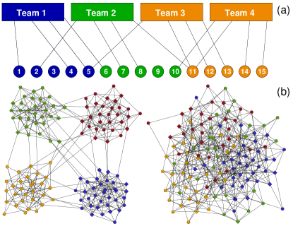
Figure 1: Model random bipartite networks with modular structure. (a) Nodes are divided into two sets, actors (circles) and teams (rectangles). Each color represents a different module in the actors’ set, and teams of a given color are more likely to contain actors of their color (see text). (b) Two sample networks with $N_{M}=4$ modules, with 16 actors (circles) each, and $N_{T}=64$ teams (diamonds), with $m=7$ actors each. The network on the left has a strong modular structure, $p=0.9$, while the modular structure is less well defined on the right, $p=0.5$ (see text for the definition of $p$).

We start by dividing the actors into $N_{M}$ of modules; each module $s$ comprises $S_{s}$ nodes. For clarity, we use different “colors” for different modules. The network is then created assuming that actors that belong to the same module have a higher probability of being together in a team than actors that belong to different modules . Specifically, we proceed by creating $N_{T}$ teams as follows:

• Create team $a$.

• Select the number $m_{a}$ of actors in the team.

• Select the color $c_{a}$ of the team, that is, the module that will contribute, in principle, the most actors to the team.

• For each spot in the team: (i) with probability $p$, select the actor from the pool of actors that have the same color as the team; (ii) otherwise, select an actor at random with equal probability. The parameter $p$, which we call team homogeneity, thus quantifies how homogeneous a team is. In the limiting cases, for $p=1$ all the actors in the team belong to the same module and modules are perfectly segregated, whereas for $p=0$ the color of the teams is irrelevant, actors are perfectly mixed and the network does not have a modular structure.

IV Results

We next investigate the performance of different module identification algorithms in both model networks with predefined modular structure, and in a simple real network that shows some interesting features.

We consider three approaches for the identification of modules in bipartite networks. First, we consider the unweighted projection (UWP) approach. Within this approach, we start by building the projection of the bipartite network into the actors space. Then we consider the projection as a regular unipartite network and use the modularity given in Eq. (1).

Next, we consider the weighted projection (WP) approach. Within this approach, we start by building the weighted projection of the bipartite network. In the weighted projection, actors are connected if they are together in one or more teams, and the weight $w_{ij}$ of the link indicates the number of teams in which the two actors are together (thus, $w_{ij}=c_{ij})$. We then use the simplest generalization to weighted networks of the modularity in Eq. (1)

$$\mathcal{M_{W}(P)}=\sum_{s=1}^{N_{M}}\left[\frac{w^{\rm int}_{s}}{W}-\left(\frac{w^{\rm all}_{s}}{2W}\right)^{2}\right]\,,$$ (6)

where $W=\sum_{i\geq j}w_{ij}$, $w^{\rm int}_{s}$ is the sum of the weights of the links within module $s$, and $w^{\rm all}_{s}=\sum_{i\in s}\sum_{j}w_{ij}$.

Finally, we consider the bipartite (B) approach. Within this approach, we consider the whole bipartite network and use the modularity introduced in Eq. (5).

In all cases, we maximize the modularity using simulated annealing Kirkpatrick et al. (1983). Several alternatives have been suggested to maximize the modularity including greedy search Newman (2004), extremal optimization Duch and Arenas (2005), and spectral methods Newman (2006a, b). In general, there is a trade-off between accuracy and execution time, with simulated annealing being the most accurate method Danon et al. (2005), but at present too slow to deal properly with networks comprising hundreds of thousands or millions of nodes.

IV.1 Model bipartite networks

We consider the performance of the different module identification approaches when applied to the model bipartite networks described above. We assess the performance of an algorithm by comparing the partitions it returns to the predefined group structure. Specifically, we use the mutual information $I_{AB}$ Danon et al. (2005) between partitions $A$ and $B$ to quantify the performance of the algorithms

$$I_{AB}=\frac{-2\sum_{i=1}^{N_{M}^{A}}\sum_{j=1}^{N_{M}^{B}}n_{ij}^{AB}\log\left(\frac{n_{ij}^{AB}S}{n_{i}^{A}n_{j}^{B}}\right)}{\sum_{i=1}^{N_{M}^{A}}n_{i}^{A}\log\left(\frac{n_{i}^{A}}{S}\right)+\sum_{j=1}^{N_{M}^{B}}n_{j}^{B}\log\left(\frac{n_{j}^{B}}{S}\right)}\,.$$ (7)

Here, $S$ is the total number of nodes in the network, $N_{M}^{A}$ is the number of modules in partition $A$, $n_{i}^{A}$ is the number of nodes in module $i$ of partition $A$, and $n_{ij}^{AB}$ is the number of nodes that are in module $i$ of partition $A$ and in module $j$ of partition $B$. The mutual information between partitions A and B is 1 if both partitions are identical, and 0 if they are uncorrelated.

In the simplest version of the model all modules have the same number of nodes, all teams have the same size, and the color of each team is set assuming equal probability for each color. Unless otherwise stated, we build networks with $N_{M}=4$ modules, each of them comprising 32 actors, and $N_{T}=128$ teams of size $m=14$.

IV.1.1 Team homogeneity

We first investigate how team homogeneity $p$ affects algorithm performance. For $p=1$, all the actors in a team belong to the same module, and any reasonable algorithm must perfectly identify the modular structure of the network; thus $I=1$. Conversely, for $p=0$, actors are perfectly mixed in teams, and all algorithms will return random partitions due to small fluctuations Guimerà et al. (2004); thus $I=0$. Any $p>0$ will provide a signal that an algorithm can, in principle, extract.

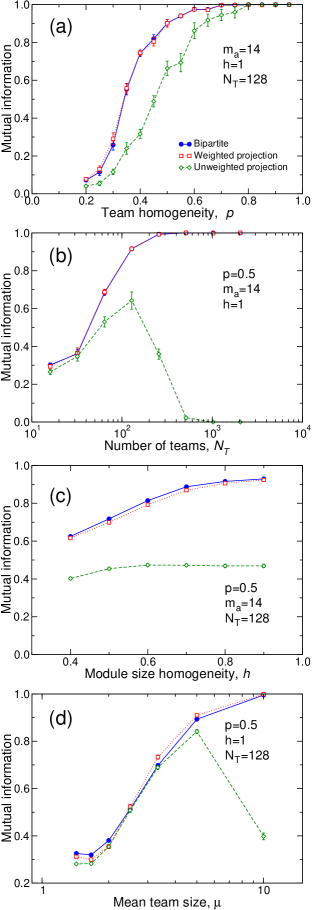
Figure 2: Algorithm performance as a function of: (a) team homogeneity $p$ (simulation parameters: $N_{M}=4$, $S_{s}=32$ for all modules); (b) number of teams $N_{T}$ (simulation parameters: $N_{M}=4$, $S_{s}=32$ for all modules); (c) module size homogeneity $h$ (simulation parameters $N_{M}=6$, $132$ nodes); and (d) mean team size $\mu$ (simulation parameters: $N_{M}=4$, $S_{s}=32$ for all modules). Error bars indicate the standard error.

As shown in Fig. 2(a), the UWP approach performs systematically and significantly worse than the weighted projection and the bipartite algorithms for all values of $p$. For the choice of parameters described above, the last two algorithms start to be able to identify the modular structure of the network for $p\approx 0.35$. For $p\geq 0.5$, one already finds $I>0.9$. The WP and the B approaches yield indistinguishable results.

IV.1.2 Number of teams and average team size

Team homogeneity is not the only parameter affecting algorithm performance. For example, the number of teams $N_{T}$ in the network critically affects the amount of information available to an algorithm. Interestingly, the number of teams affects in different ways the UWP approach on the one hand, and the WP and B approaches on the other; Fig. 2(b). For the WP and B algorithms, the larger $N_{T}$, the larger the amount of information and therefore the easier the problem becomes. Indeed, even for very small values of $p$, the signal to noise ratio can become significantly greater than 1 if $N_{T}$ is large enough. On the contrary, as the number of teams increases the UWP becomes denser and denser and eventually becomes a fully connected graph, from which the algorithm cannot extract any useful information. Once more, the performance of the WP and the B approaches are indistinguishable.

IV.1.3 Module size heterogeneity

In real networks, modules will have (sometimes dramatically) different sizes Danon et al. (2006). Given the sizes of the modules in a network, and assuming that they are ordered so that $S_{1}\geq S_{2}\geq\dots\geq S_{N_{M}}$, we define $h$ as the ratio of sizes between consecutive modules (with integer rounding)

$$h=\frac{S_{i+1}}{S_{i}}\,.$$ (8)

Additionally, we select the color of the teams with probabilities proportional to the size of the corresponding module, so that all actors participate, on average, in the same number of teams.

As we show in Fig. 2(c), we again observe that the WP and the B approach perform similarly, and clearly outperform the UWP approach for all values of $h$.

IV.1.4 Team size distribution

All the results so far suggest that the WP approach and the B approach yield results that are indistinguishable from each other. We know, however, that differences do exist between both. The distribution of team sizes, in particular, is taken into account in the B approach but disregarded in the WP approach, and “teams” with $m=1$ are totally disregarded in projection-based approaches, but not in the B approach.

We thus investigate what is the effect of the team size distribution on the performance of the algorithms. Instead of considering that all teams have the same size $m$, we now consider a distribution $p(m)$ of team sizes. In particular, we consider a (displaced) geometric distribution

$$p(m)=\frac{1}{\mu}\left(1-\frac{1}{\mu}\right)^{m-1}\quad,\quad m\geq 1\,,$$ (9)

which is the discrete counterpart of the exponential distribution. The distribution has mean $\langle m\rangle=\mu$.

As we show in Fig. 2(d), some small differences seem to appear between the WP approach and the B approach, although it is difficult to establish conclusively if these differences are significant or not.

In the light of this, we investigate in more depth the relationship between the bipartite modularity in Eq. (5) and the weighted extension of the unipartite modularity in Eq. (1). As we show in the Appendix, the bipartite modularity actually reduces to the weighted unipartite modularity (up to an irrelevant additive constant) when all teams in the bipartite network have the same size.

This observation explains why the WP and the B approach differ when teams have unequal sizes . Although our results suggest that each approach outperforms the other in certain cases, we believe that Eq. (5) is, in general, preferable because it explicitly takes into account the distribution of team sizes, while the weighted projection does not.

IV.2 Southern women dataset

During the 1930s, ethnographers Allison Davis, Elizabeth Stubbs Davis, J. G. St. Clair Drake, Burleight B. Gardner, and Mary R. Gardner collected data on social stratification in the town of Natchez, Mississippi Davis et al. (1941); Freenan (2003). Part of their field work consisted in collecting data on women’s attendance to social events in the town. The researchers later analyzed the resulting women-event bipartite network in the light of other social and ethnographic variables. Since then, the dataset has become a de facto standard for discussing bipartite networks in the social sciences Freenan (2003).

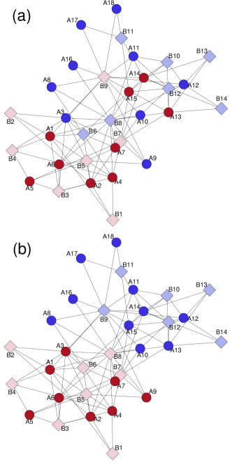
Figure 3: Modular structure of the Southern women dataset Davis et al. (1941); Freenan (2003). Circles represent women and diamonds represent social events. A woman and an event are connected if the woman attended the event. (a) Modular structure as obtained from the unweighted projection (UWP) approach. (b) Modular structure as obtained from the weighted projection (WP) approach and the bipartite (B) approach. The UWP approach fails to capture the real modular structure of the network.

Here we analyze the modules of both women and events. We start by considering the unweighted projection of the network in the women’s space (two women are connected if they co-attended at least one event), and in the events’ space (two events are connected if at least one woman was in both events). As we show in Fig. 3(a), the unweighted projection does not capture the true modular structure of the network. The failure of this approach is due to the fact that the projections are very dense. For example, some central events were attended by most women and thus most pairs of women are connected in the projection.

As we show in Fig. 3(b), the weighted projection approach and the bipartite approach yield the exact same results, which do capture the two-module structure of the network. Except for one woman, the partition coincides with the original subjective partition proposed by the ethnographers who collected the data, and is in perfect agreement with some of the supervised algorithms reviewed in Ref. Freenan (2003).

V Modules in directed networks

Another important class of networks for which no satisfactory module identification algorithm has so far been proposed is directed unipartite networks. In order to tackle this class of networks, we note that directed networks can be conveniently represented as bipartite networks where each node $i$ is represented by two nodes $A_{i}$ and $B_{i}$. A directed link from $i$ to $j$ would be represented in the bipartite network as an edge connecting $A_{i}$ to $B_{j}$.

Consider, for example, a network in which nodes are companies and links represent investments of one company into another. By considering each company as two different objects, one that makes investments and one that receives investments, the directed network can be represented as an undirected bipartite network. Modules in the set of objects that make investments correspond to groups of companies that invest in the same set of companies, that is, groups of companies with a similar investing strategy.

The most widely used approach to identify communities in directed networks is to simply disregard the directionality of the links and identify modules using a method suitable for undirected unipartite networks. This method might work in some situations, but will fail when different modules are defined based on incoming and outgoing links.

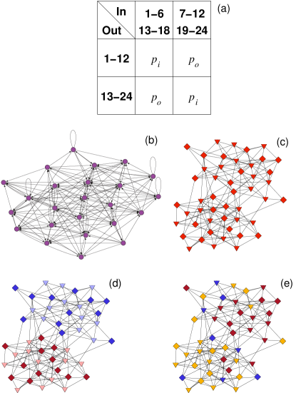
Figure 4: Application of the bipartite approach to the identification of modules in directed networks. (a, b) A directed model network. A link from node $i$ to node $j$ is established according to the probabilities in the matrix in (a). For example, there is a probability $p_{i}$ that there is a link from node 1 to node 13. In particular, we use $p_{i}=0.45>p_{o}=0.05$ to generate the directed network in (b). (c) Bipartite representation of the network in (b). Each node $i$ is in (b) is represented by two nodes here, a circle $A_{i}$ and a square $B_{i}$. All links in the bipartite network run between circles and diamonds, and a link between $A_{i}$ and $B_{j}$ corresponds to a link from $i$ to $j$ in the directed network. (d) Modules identified in the bipartite network. (e) Modules identified from the directed network disregarding link direction. Here, we use the same color for $A_{i}$ and $B_{i}$, since this approach does not make distinctions between incoming and outgoing links.

Consider, for instance, the simple model network depicted in Figs. 4(a, b). According to the outgoing links of the nodes this network has two modules: nodes 1-12 and nodes 13-24. According to the incoming links of the nodes the network has also two modules, but they are different: nodes 1-6 and 13-18 on the one hand, and nodes 7-12 and 19-24 on the other. As we show in Fig. 4(c), a layout of the corresponding bipartite network already makes clear the modular structure of the network, and any of the approaches described above (UWP, WP, and B) is able to identify the in-modules and out-modules correctly; Fig. 4(d). Disregarding the direction of the links, however, results in modules that fail to capture the modular structure of the network; Fig. 4(e).

VI Discussion

In this work, we have focused on approaches that aim at identifying modules in each of the two sets of nodes in the bipartite network independently. There are two main reasons for this choice. First, methodologically our choice enables comparison with projection-based algorithms, which, by definition, cannot identify modules of actors and teams simultaneously. Second, in most situations it is reasonable to assume that two actors belong to the same module if they co-participate in many teams, regardless of whether the teams themselves belong to the same module or not. An alternative approach, however, would be to group nodes in both sets at the same time.

Another interesting observation relates to the optimization algorithm used to maximize the modularity. Although we have chosen to use simulated annealing to obtain the best possible accuracy Guimerà and Amaral (2005a, b); Danon et al. (2005), one can trivially use the new modularity introduced in Eq. (5) with faster algorithms such as greedy search Newman (2004) or extremal optimization Duch and Arenas (2005).

Interestingly, one can also use the spectral methods introduced in Newman (2006a, b). Indeed, just as the unipartite modularity $\mathcal{M}(P)$, the bipartite modularity $\mathcal{M_{B}(P)}$ can be rewritten in matrix form as

$$\mathcal{M_{B}(P)}=\mathbf{g^{T}Bg}\,,$$ (10)

where $g_{is}=1$ if node $i$ belongs to module $s$ and 0 otherwise, and the elements of the modularity matrix $\mathbf{B}$ are defined as

$$B_{ij}=\left\{\begin{array}[]{ll}\frac{c_{ij}}{\sum_{a}m_{a}(m_{a}-1)}-\frac{t_{i}t_{j}}{\left(\sum_{a}m_{a}\right)^{2}}&i\neq j\\ 0&i=j\end{array}\right..$$ (11)

Even more importantly, by sampling all local maxima of the modularity in Eq. (5) one can study, not only the most modular partition of the network, but the hierarchical structure of nested modules and submodules Sales-Pardo et al. (2007) within each set of nodes in the bipartite network. This is particularly relevant taking into account that the most modular partition of a network may, in some cases, not represent the most “relevant” division of its nodes Fortunato and Barthélemy (2007); Sales-Pardo et al. (2007).

Finally, a few words are necessary on the comparison between the different approaches. First, we have shown that the (so far “default”) unweighted projection approach is not reliable and can lead, in most situations, to incorrect results. Therefore, we believe that this approach should not be used. As for the weighted projection approach and the bipartite approach, we have shown that their performance is very similar, and that they are actually equivalent when all teams in the bipartite network have the same size. We have also pointed out, however, that they can and do give noticeably different results when team sizes are not uniform. Given this, we believe that the bipartite approach has a more straightforward interpretation and would be preferable in cases in which the modular structure of the network is unknown.

Appendix A Weighted unipartite modularity and bipartite modularity for bipartite networks with uniform teams

Next, we demonstrate that, when all teams in a bipartite network have the same size $m$, the bipartite modularity is equivalent to the modularity of the weighted projection.

We consider the usual weighted projection, in which each pair of nodes $i\neq j$ is connected by a link whose weight $w_{ij}$ equals the number of times that $i$ and $j$ are together in a team; using our previous notation $w_{ij}=c_{ij}$. No self-links are included in the projection.

In this projection, and when all teams have the same number of actors $m_{a}\equiv m$, the constant team-size factors in Eq. (5) become

$$\sum_{a}m_{a}(m_{a}-1) = N_{T}m(m-1)=2W$$ (12)

$$\left(\sum_{a}m_{a}\right)^{2} = \left(\frac{2W}{m-1}\right)^{2}\,$$ (13)

where, as before, $W=\sum_{i\geq j}w_{ij}$.

Each time an actor is in a team, the total weight of the links in the projected network increases by $(m-1)$. Using this and the identities above, we obtain

$$\frac{\sum_{i\neq j\in s}c_{ij}}{\sum_{a}m_{a}(m_{a}-1)} = \frac{w^{\rm int}_{s}}{W}$$ (14)

$$\frac{\sum_{i\neq j\in s}t_{i}t_{j}}{\left(\sum_{a}m_{a}\right)^{2}} = \sum_{i\in s}\frac{(m-1)t_{i}}{2W}\sum_{j\in s,j\neq i}\frac{(m-1)t_{j}}{2W}$$ (16)

$$= \left(\frac{w_{s}^{\rm all}}{2W}\right)^{2}-$$

$$\sum_{i\in s}\left(\frac{(m-1)t_{i}}{2W}\right)^{2}\,.$$

Once the summation over modules is carried out, the last term is simply a constant independent of the partition, and is therefore irrelevant. Thus, up to an irrelevant constant, when all teams in a bipartite network have the same size, the bipartite modularity in Eq. (5) is equivalent to the weighted modularity in Eq. (6).

References

- Albert and Barabási (2002) R. Albert and A.-L. Barabási, Rev. Mod. Phys. 74, 47 (2002).
- Newman (2003) M. E. J. Newman, SIAM Review 45, 167 (2003).
- Amaral and Ottino (2004) L. A. N. Amaral and J. Ottino, Eur. Phys. J. B 38, 147 (2004).
- Girvan and Newman (2002) M. Girvan and M. E. J. Newman, Proc. Natl. Acad. Sci. USA 99, 7821 (2002).
- Guimerà et al. (2005a) R. Guimerà, S. Mossa, A. Turtschi, and L. A. N. Amaral, Proc. Natl. Acad. Sci. USA 102, 7794 (2005a).
- Colizza et al. (2006a) V. Colizza, A. Barrat, M. Barthélemy, and A. Vespignani, Proc. Natl. Acad. Sci. USA 103, 2015 (2006a).
- Pastor-Satorras and Vespignani (2001) R. Pastor-Satorras and A. Vespignani, Phys. Rev. Lett. 86, 3200 (2001).
- Liljeros et al. (2003) F. Liljeros, C. R. Edling, and L. A. N. Amaral, Microbes Infect. 5, 189 (2003).
- Guimerà et al. (2007) R. Guimerà, M. Sales-Pardo, and L. A. N. Amaral, Nature Phys. 3, 63 (2007).
- Newman (2002) M. E. J. Newman, Phys. Rev. Lett. 89, art. no. 208701 (2002).
- Pastor-Satorras et al. (2001) R. Pastor-Satorras, A. Vázquez, and A. Vespignani, Phys. Rev. Lett. 87, art. no. 258701 (2001).
- Maslov and Sneppen (2002) S. Maslov and K. Sneppen, Science 296, 910 (2002).
- Maslov et al. (2004) S. Maslov, K. Sneppen, and A. Zaliznyak, Physica A 333, 529 (2004).
- Colizza et al. (2006b) V. Colizza, A. Flammini, M. A. Serrano, and A. Vespignani, Nature Phys. 2, 110 (2006b).
- Danon et al. (2005) L. Danon, A. Díaz-Guilera, J. Duch, and A. Arenas, J. Stat. Mech.: Theor. Exp. p. art. no. P09008 (2005).
- Borgatti and Everett (1997) S. P. Borgatti and M. G. Everett, Social Networks 19, 243 (1997).
- Doreian et al. (2004) P. Doreian, V. Batagelj, and A. Ferligoj, Social Networks 26, 29 (2004).
- Uetz et al. (2000) P. Uetz, L. Giot, G. Cagney, T. A. Mansfield, R. S. Judson, J. R. Knight, D. Lockshon, V. Narayan, M. Srinivasan, P. Pochart, et al., Nature 403, 623 (2000).
- Jeong et al. (2001) H. Jeong, S. P. Mason, A.-L. Barabási, and Z. N. Oltvai, Nature 411, 41 (2001).
- Li et al. (2004) S. Li, C. M. Armstrong, N. Bertin, H. Ge, S. Milstein, M. Boxem, P.-O. Vidalain, J.-D. J. Han, A. Chesneau, T. Hao, et al., Science 303, 540 (2004).
- Jordano (1987) P. Jordano, Am. Nat. 129, 657 (1987).
- Bascompte et al. (2003) J. Bascompte, P. Jordano, C. J. Meli n, and J. M. Olesen, Proc. Natl. Acad. Sci. U. S. A. 100, 9383 (2003).
- Newman (2001) M. E. J. Newman, Proc. Natl. Acad. Sci. USA 98, 404 (2001).
- Börner et al. (2004) K. Börner, J. T. Maru, and R. L. Goldstone, Proc. Natl. Acad. Sci. USA 101, 5266 (2004).
- Guimerà et al. (2005b) R. Guimerà, B. Uzzi, J. Spiro, and L. A. N. Amaral, Science 308, 697 (2005b).
- Gleiser and Danon (2003) P. M. Gleiser and L. Danon, Adv. Complex Syst. 6, 565 (2003).
- Uzzi and Spiro (2005) B. Uzzi and J. Spiro, Am. J. Sociol. 111, 447 (2005).
- Stouffer et al. (2005) D. B. Stouffer, J. Camacho, R. Guimerà, C. A. Ng, and L. A. N. Amaral, Ecology 86, 1301 (2005).
- Williams and Martinez (2000) R. J. Williams and N. D. Martinez, Nature 404, 180 (2000).
- Barabási and Oltvai (2004) A.-L. Barabási and Z. N. Oltvai, Nat. Rev. Genet. 5, 101 (2004).
- Everitt et al. (2001) B. S. Everitt, S. Landau, and M. Leese, Cluster Analysis (Arnold Pub., 2001).
- Freenan (2003) L. C. Freenan, in Dynamic Social Network Modeling and Analysis: Workshop Summary and Papers, edited by R. Breiger, C. Carley, and P. Pattison (The National Academies Press, Washington, DC, 2003), pp. 39–97.
- Fortunato and Barthélemy (2007) S. Fortunato and M. Barthélemy, Proc. Natl. Acad. Sci. USA 104, 36 (2007).
- Sales-Pardo et al. (2007) M. Sales-Pardo, R. Guimerà, A. A. Moreira, and L. A. N. Amaral, arXiv:0705.1679 (2007).
- Fortunato (2007) S. Fortunato, arXiv:0705.4445 (2007).
- Guimerà and Amaral (2005a) R. Guimerà and L. A. N. Amaral, Nature 433, 895 (2005a).
- Guimerà and Amaral (2005b) R. Guimerà and L. A. N. Amaral, J. Stat. Mech.: Theor. Exp. p. art. no. P02001 (2005b).
- Guimerà et al. (2004) R. Guimerà, M. Sales-Pardo, and L. A. N. Amaral, Phys. Rev. E 70, art. no. 025101 (2004).
- Reichardt and Bornholdt (2006) J. Reichardt and S. Bornholdt, Phys. Rev. E 74, 016110 (2006).
- Newman and Girvan (2004) M. E. J. Newman and M. Girvan, Phys. Rev. E 69, art. no. 026113 (2004).
- Kirkpatrick et al. (1983) S. Kirkpatrick, C. D. Gelatt, and M. P. Vecchi, Science 220, 671 (1983).
- Newman (2004) M. E. J. Newman, Phys. Rev. E 69, art. no. 066133 (2004).
- Duch and Arenas (2005) J. Duch and A. Arenas, Phys. Rev. E 72, art. no. 027104 (2005).
- Newman (2006a) M. E. J. Newman, Proc. Natl. Acad. Sci. USA 103, 8577 (2006a).
- Newman (2006b) M. E. J. Newman, Phys. Rev. E 74, art. no. 036104 (2006b).
- Danon et al. (2006) L. Danon, A. Díaz-Guilera, and A. Arenas, J. Stat. Mech.: Theor. Exp. p. P11010 (2006).
- Davis et al. (1941) A. Davis, B. B. Gardner, and M. R. Gardner, Deep South (University of Chicago Press, Chicago, 1941).