Fully developed turbulent dynamo at low magnetic Prandtl numbers.

Abstract

We investigate the dynamo problem in the limit of small magnetic Prandtl number ($\mathrm{Pm}$) using a shell model of magnetohydrodynamic turbulence. The model is designed to satisfy conservation laws of total energy, cross helicity and magnetic helicity in the limit of inviscid fluid and null magnetic diffusivity. The forcing is chosen to have a constant injection rate of energy and no injection of kinetic helicity nor cross helicity. We find that the value of the critical magnetic Reynolds number ($\mathrm{Rm}$) saturates in the limit of small $\mathrm{Pm}$. Above the dynamo threshold we study the saturated regime versus $\mathrm{Rm}$ and $\mathrm{Pm}$. In the case of equipartition, we find Kolmogorov spectra for both kinetic and magnetic energy except for wave numbers just below the resistive scale. Finally the ratio of both dissipation scales (viscous to resistive) evolves as $\mathrm{Pm}^{-3/4}$ for $\mathrm{Pm}<1$.

1 Introduction

Most of astrophysical bodies possess or have had in their history their own magnetic fields. In most cases their generation rely on inductive processes produced by the turbulent motion of the electroconducting fluid within the body [1]. An important parameter of the problem is the magnetic Prandtl number defined by $\mathrm{Pm}=\nu/\eta$ where $\nu$ is the viscosity and $\eta$ the magnetic diffusivity of the fluid. In the “magnetic” universe $\mathrm{Pm}$ varies from values as large as $10^{14}$ for the interstellar medium [2] to values as small as $10^{-6}$ for the iron core of planets or stellar plasmas. This large spectrum of possible $\mathrm{Pm}$ values implies strong differences between possible generation mechanisms. In some sense $\mathrm{Pm}$ is a measure of the kinetic energy spectrum available for generating magnetic energy. When $\mathrm{Pm}\geq 1$ the resistive scale is smaller than the viscous scale implying that all velocity scales are available for generating some magnetic field. In the other hand for $\mathrm{Pm}<1$, only the velocity scales larger than the resistive scale are available for the magnetic field generation. In that case, the velocity scales smaller than the resistive scale are enslaved to the larger scales and in essence they stay passive in the generation process. Besides this is why the large eddy simulation technique may be recommended in that case [3]. Therefore, at first sight one can expect that dynamo action is all the more difficult to obtain since $\mathrm{Pm}$ is smaller in reason of a smaller velocity spectrum available for the magnetic generation. This is indeed what comes out from recent numerical simulations [4, 5, 6, 7, 8, 9] (see also [10] and references therein for an alternative approach). Though, we have evidence of magnetic field in planets and stars, and dynamo action has also been reproduced in experiments working with liquid sodium for which $\mathrm{Pm}$ is small ($\sim 10^{-6}$) [11, 12, 13, 14]. These experiments and further devices in preparation [15, 16, 17] are designed in such a way that the dynamo mechanism is produced by the large scale of the flow due to an appropriate large scale forcing. The turbulence naturally developing at smaller scales may play a role though this is still unclear [18, 19, 3, 20, 21]. In these experiments, the choice of the forcing is based on the hypothesis that it is the stationary part of the large scale flow which should be important for the generation mechanism. A number of flow geometries studied in the past turned out to be good candidates for such experiments [22, 23, 24].

In the present paper we are interested in the possibility for a Kolmogorov type turbulent flow to generate dynamo action at low $\mathrm{Pm}$, without need for a large scale motion controlling the generation mechanism. We expect the eddies having the highest shearing rate to be the more active for generating the magnetic field, at least during the kinematic stage of magnetic field growth. As in Kolmogorov turbulence $u_{l}/l\approx l^{-2/3}$, these eddies correspond to the smallest available scale which is the viscous scale for $\mathrm{Pm}\geq 1$ [25] and the resistive scale for $\mathrm{Pm}<1$ [9]. Eventually the magnetic field will then spread out to larger scales due to the nonlinear interactions. This problem is hard to solve by direct numerical simulation for it needs high resolution in order to describe magnetic phenomena adequately [26]. Some results have been obtained using the EDQNM closure applied to the MHD equations [27] near the critical $\mathrm{Rm}$ and for arbitrary low values of $\mathrm{Pm}$. Here we want to investigate arbitrary large values of $\mathrm{Rm}$ and small values of $\mathrm{Pm}$. For that we use a shell model of MHD turbulence introduced by Frick and Sokoloff [28]. This model is the successor of several other shell models for MHD turbulence [29, 30, 31, 32, 33, 34, 35] but it is the only one to conserve all integrals of motions including magnetic helicity (or kinetic helicity for the non magnetic case). It is based on the so-called GOY hydrodynamic shell model [36, 37, 38, 39]. In [28], Frick and Sokoloff have derived a model which represents either 2D or 3D MHD turbulence, depending on the choice of two parameters. As in real MHD turbulence the 2D model leads to the impossibility of dynamo action [40]. This shows that in spite that such a shell model is a drastic simplification of the real MHD turbulence, ignoring for example the geometrical structures of the motion and magnetic field, it contains enough features to make the difference between the 2D and 3D problems (see also [41]). It also reproduces quite well the structure functions at different orders of real MHD turbulence. Here we consider only the 3D model herein after referred to as FS98. This model has also been used by Lozhkin et al. [42] to show that small scale dynamo is possible at low $\mathrm{Pm}$, contrary to the hypothesis put forward by Batchelor [43].

Giulani and Carbone [41] have shown that long runs with the FS98 model lead inevitably towards a “dynamical alignement” stopping the nonlinear transfer towards the smaller scales. Giulani and Carbone [41] suggested that this problem might be overcome with an other choice of the external driving force. This is what we have done here, adopting a forcing in such a way that it acts on several scales and depends on time with a random phase at each forcing scale (see section 2.2). Finally, we took care to have long runs well beyond any transient state, in order to have good statistics and reliable results.

2 Shell model for MHD turbulence

2.1 Model equations

The shell model is built up by truncation of the Navier-Stokes and induction equations. We define logarithmic shells, each shell being characterized by one real wave number $k_{n}=k_{0}\lambda^{n}$ and dynamical complex quantities $U_{n}$ and $B_{n}$ representative of the velocity and magnetic fluctuations for wave vectors of norm ranging between $k_{n}$ and $k_{n+1}$. The parameter $\lambda$ is taken equal to the gold number $(1+\sqrt{5})/2$ for it optimizes the resolution [44]. The model is described by the following set of equations ($0\leq n\leq N$)

$$d_{t}U_{n} = ik_{n}(Q_{n}(U,U,a)-Q_{n}(B,B,a))$$ (1)

$$- \nu k_{n}^{2}U_{n}+F_{n},$$

$$d_{t}B_{n} = ik_{n}(Q_{n}(U,B,b)-Q_{n}(B,U,b))$$ (2)

$$- \eta k_{n}^{2}B_{n},$$

where

$$Q_{n}(X,Y,c) = c_{1}X_{n+1}^{*}Y_{n+2}^{*}+c_{2}X_{n-1}^{*}Y_{n+1}^{*}$$ (3)

$$+ c_{3}X_{n-2}^{*}Y_{n-1}^{*}.$$

represents the nonlinear transfer rates with the four neighbouring shells $n-2$, $n-1$, $n+1$ and $n+2$. In addition we have to take $U_{-2}=U_{-1}=U_{N+1}=U_{N+2}=0$ and $B_{-2}=B_{-1}=B_{N+1}=B_{N+2}=0$. The parameter $F_{n}$ is the forcing at shell $n$. The time unit is defined by the turnover time of the largest scale $\tau=(|U_{0}|k_{0})^{-1}$. To determine the complex coefficients $a_{j}$ and $b_{j}$, $j=1,2,3$ we apply the property that the total energy $E_{tot}$, cross-helicity ${\cal H}_{C}$ and magnetic helicity ${\cal H}_{B}$ must be conserved in the limit of non-viscous and non-resistive limit $\nu=\eta=0$. In our shell model, these quadratic quantities write in the following form

$$E_{tot} = \frac{1}{2}\sum_{n=0}^{N}(|U_{n}|^{2}+|B_{n}|^{2}),$$ (4)

$${\cal H}_{C} = \frac{1}{2}\sum_{n=0}^{N}(U_{n}B_{n}^{*}+B_{n}U_{n}^{*}),$$ (5)

$${\cal H}_{B} = \frac{1}{2}\sum_{n=0}^{N}(-1)^{n}|B_{n}|^{2}/k_{n},$$ (6)

leading to $a_{1}=1$, $a_{2}=(1-\lambda)\lambda^{-2}$, $a_{3}=-\lambda^{-3}$, $b_{1}=b_{2}=b_{3}=(\lambda(1+\lambda))^{-1}$. In the pure hydrodynamic case ($B_{n}=0$) the original GOY model is recovered satisfying, in addition to (4), the conservation of the kinetic helicity [45]

$${\cal H}_{U}=\frac{1}{2}\sum_{n=0}^{N}(-1)^{n}|U_{n}|^{2}k_{n}.$$ (7)

2.2 Forcing and initial conditions

The forcing is chosen in order to control the injection rate of kinetic energy, cross and kinetic helicities. For that we spread the forcing on three neighbouring shells $n_{f},n_{f}+1$ and $n_{f}+2$ with $F_{n_{f}+j}=f_{j}e^{i\phi_{j}}$, $j=0,1,2$ where the $f_{j}$ are positive real quantities and where the $\phi_{j}\in\left[0,2\pi\right]$ are random phases. In that case the forcing is $\delta$-correlated. Alternatively we also used a forcing for which the phases $\phi_{j}$ are constant during a certain time $\tau_{c}$, which can be interpreted as a finite correlation time. In fact this does not make much difference either on the autocorrelation functions of $U_{n}$ nor on the subsequent results. Therefore it is sufficient to use random phases. As we are interested to inject neither kinetic helicity nor cross-helicity, the forcing functions must satisfy

$$\frac{1}{2}\sum_{n=n_{f}}^{n_{f}+2}U_{n}^{*}F_{n}+U_{n}F_{n}^{*}=\varepsilon,$$ (8)

$$\sum_{n=n_{f}}^{n_{f}+2}(-1)^{n}k_{n}(U_{n}^{*}F_{n}+U_{n}F_{n}^{*})=0,$$ (9)

$$\sum_{n=n_{f}}^{n_{f}+2}B_{n}^{*}F_{n}+B_{n}F_{n}^{*}=0.$$ (10)

where $\varepsilon$ is the rate of kinetic energy supplied to the system. Therefore for a given set of random $\phi_{j}$ ($j=0,1,2$), the $f_{j}$ depend on the $U_{j}$ and $B_{j}$ ($j=0,1,2$) which expressions are given in Appendix. For some arbitrary initial conditions on $U_{j}$ ($j=0,1$) of small intensity ($\sim 10^{-6}$) we let the hydrodynamic evolve until it reaches some statistically stationary state. Then introducing at a given time some arbitrary non zero values of $B_{j}$ ($j=0,1$) of small intensity ($\sim 10^{-6}$) we solve the full problem until a statistically stationary MHD state is reached. The time of integration needed to obtain good statistics depends on $\nu$ and $\eta$ but typically it is equal to several hundreds of the large scale turn-over time.

2.3 Input and output

The input parameters of the problem are $\nu$, $\eta$, the forcing shell $n_{f}$, the rate of injected kinetic energy $\varepsilon$ and the number of shells $N$. In the rest of the paper we take $\varepsilon=1$.

As output we define the kinetic and magnetic energy for the shell $n$ by

$$E^{U}(n)=\frac{1}{2}|U_{n}|^{2}\quad\mbox{and}\quad E^{B}(n)=\frac{1}{2}|B_{n}|^{2},$$ (11)

the total kinetic and total magnetic energy by

$$E_{U}=\sum_{n=0}^{N}E^{U}(n)\quad\mbox{and}\quad E_{B}=\sum_{n=0}^{N}E^{B}(n)$$ (12)

and the total energy by

$$E_{tot}=E_{U}+E_{B}.$$ (13)

Following [46] we define the spectral energy fluxes from the inside of the $U$(or $B$)-sphere (shells with $k<k_{n}$) to the outside of the $U$(or $B$)-sphere (shells with $k\geq k_{n}$). We note for example $\Pi_{U>}^{B<}(n)$ the energy flux from the inside of the $B$-sphere to the outside of the $U$-sphere. Then we have

$$\Pi_{U>}^{U<}(n) = \sum^{n-1}_{j=0}\Im\{k_{j}U_{j}^{*}Q_{j}(U,U,a)\}$$ (14)

$$\Pi_{U>}^{B<}(n) = \sum^{n-1}_{j=0}\Im\{-k_{j}U_{j}^{*}Q_{j}(B,B,a)\}$$ (15)

$$\Pi_{B>}^{U<}(n) = \sum^{n-1}_{j=0}\Im\{-k_{j}B_{j}^{*}Q_{j}(B,U,b)\}$$ (16)

$$\Pi_{B>}^{B<}(n) = \sum^{n-1}_{j=0}\Im\{k_{j}B_{j}^{*}Q_{j}(U,B,b)\}.$$ (17)

In FS98 the time average of $\Pi_{U>}^{U<}(n)$ is denoted $\Pi_{n}$. We also define the energy fluxes from the inside of the $U$-and-$B$-spheres to the outside of the $U$-sphere or $B$-sphere by

$$\Pi_{U}(n) = \Pi_{U>}^{U<}(n)+\Pi_{U>}^{B<}(n)$$ (18)

$$\Pi_{B}(n) = \Pi_{B>}^{U<}(n)+\Pi_{B>}^{B<}(n)$$ (19)

and the total energy flux by

$$\Pi_{tot}(n) = \Pi_{U}(n)+\Pi_{B}(n).$$ (20)

We define the viscous and resistive dissipation rates $D^{U}(n)$ and $D^{B}(n)$ in shell $n$, by

$$D^{U}(n) = \nu k_{n}^{2}|U_{n}|^{2}$$ (21)

$$D^{B}(n) = \eta k_{n}^{2}|B_{n}|^{2}$$ (22)

and the total dissipation rate by

$$D_{tot}=\sum_{n=0}^{N}(D^{U}(n)+D^{B}(n)).$$ (23)

With these definitions we obtain the following shell-by-shell energy budget equations:

$$d_{t}\sum_{j=0}^{n}E^{U}(j)+\Pi_{U}(n) = -\sum_{j=0}^{n}D^{U}(j)+\epsilon$$ (24)

$$d_{t}\sum_{j=0}^{n}E^{B}(j)+\Pi_{B}(n) = -\sum_{j=0}^{n}D^{B}(j).$$ (25)

For a statistical stationary solution ($d_{t}\langle E^{U}(j)\rangle=d_{t}\langle E^{B}(j)\rangle=0$) we have then

$$\langle\Pi_{tot}(n)\rangle = -\sum_{j=0}^{n}\langle D^{U}(j)\rangle-\sum_{j=0}^{n}\langle D^{B}(j)\rangle+\epsilon.$$ (26)

where here and after $\langle\quad\rangle$ denotes time averaged quantities.

We define the kinetic and magnetic Reynolds numbers as

$$\mathrm{Re} = \langle E_{tot}\rangle^{2}/(\nu\langle D_{tot}\rangle)$$ (27)

$$\mathrm{Rm} = \langle E_{tot}\rangle^{2}/(\eta\langle D_{tot}\rangle).$$ (28)

Finally, following [47], we define the viscous (resp. resistive) scale $k_{\nu}^{-1}$ (resp. $k_{\eta}^{-1}$) as the one at which the viscous (resp. Ohmic) decay time $\tau_{\nu}=(\nu k_{n}^{2})^{-1}$ (resp. $\tau_{\eta}=(\eta k_{n}^{2})^{-1}$) becomes comparable to the typical turn-over time $\tau_{U}=(k_{n}\langle|U_{n}|^{2}\rangle^{1/2})^{-1}$.

3 Hydrodynamics

Choosing the appropriate forcing corresponding to $B_{n}=0$ we present in Fig.1 some results concerning the pure hydrodynamic case for $\nu=10^{-8}$ and $n_{f}=8$.

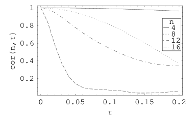
(a)	(b)
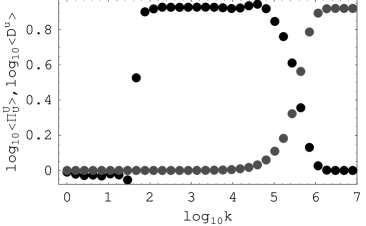
(c)	(d)

Figure 1: Hydrodynamic case for $\nu=10^{-8}$ and a forcing scale (arrow) corresponding to $n_{f}=8$. The output Reynolds number is $\mathrm{Re}=8\;10^{7}$. In (a), the autocorrelation function $cor(n,\tau)$ for a $\delta$-correlated forcing is plotted versus $\tau$ and for several shells $n$. In (c), the turn-over (black dots) and dissipation (straight line) characteristic times are plotted versus $\log_{10}k$. In (b), the energy spectrum is plotted versus $\log_{10}k$ and the $k^{-2/3}$ slope (full line) is plotted for comparison. In (d), the energy flux (black dots) and the dissipation $\sum_{j=0}^{n}D^{U}(j)$ (gray dots) are plotted versus $\log_{10}k$.

In this case the forcing is $\delta$-correlated. Though the autocorrelation function, defined by

$$cor(n,\tau)=\frac{\int U_{n}^{*}(t)U_{n}(t+\tau)+U_{n}(t)U_{n}^{*}(t+\tau)dt}{2\sqrt{\int U_{n}^{*}(t)U_{n}(t)dt\int U_{n}(t+\tau)U_{n}^{*}(t+\tau)dt}}$$ (29)

and plotted in Fig.1a, is far from being the one of a $\delta$-correlated velocity contrary to the Kasantzev model [9]. We also made comparisons with a finite correlation time forcing without finding any significant differences. Therefore the $\delta$-correlated forcing does not seem to be an issue in our problem.

The kinetic energy spectrum (Fig.1b, black dots) of the stationary statistical state is found to be in $k^{-2/3}$ (which corresponds to a Fourier energy spectrum of $k^{-5/3}$ as expected in Kolmogorov turbulence). In Fig.1c, the spectral flux $\Pi_{U}(n)$ (black dots) and the dissipation $\sum_{j=0}^{n}D^{U}(j)$ (gray dots) are found to satisfy the kinetic energy budget (24) with $\epsilon=1$. In addition, in the inertial range we find that $\Pi_{U}(n)\sim\epsilon$ and $\sum_{j=0}^{n}D^{U}(j)\sim 0$ as predicted by a Kolmogorov turbulence. After the viscous scale, $\Pi_{U}(n)\sim 0$ and $\sum_{j=0}^{n}D^{U}(j)\sim\epsilon$.

As previously defined, the viscous scale is the one at which the viscous decay time $\tau_{\nu}=(\nu k_{n}^{2})^{-1}$ (full curve of Fig.1c) becomes comparable to the typical turn-over time $\tau_{U}=(k_{n}U_{n})^{-1}$ (black dots of Fig.1c). This leads to $k_{\nu}\sim 10^{6}$ and compares indeed very well with the Kolmogorov dissipation scale $k_{\nu}^{-1}\sim(\nu^{3}/\epsilon)^{1/4}$. Finally the little bump of $\Pi_{U}(n)$ (black dots Fig.1d) just before the viscous scale looks like a bottle-neck effect [48].

4 Dynamo action

4.1 Time evolution of quadratic quantities

(a)	(b)	(c)
(d)	(e)	(f)

Figure 2: Quadratic quantities (a) $E_{tot}$, (b) $E_{U}$, (c) $E_{B}$, (d) ${\cal H}_{U}$, (e) ${\cal H}_{B}$ and (f) ${\cal H}_{C}/\sqrt{E_{U}E_{B}}$ versus time, for $\nu=10^{-9}$ and $\eta=10^{-6}$.

Here we start with a typical example of magnetic generation for $\nu=10^{-9}$ and $\eta=10^{-6}$ ($\mathrm{Pm}=10^{-3}$). In Fig. 2 the different quadratic quantities defined in (4), (5), (6), (7) and (12) are plotted versus time. A coarse time sampling has been chosen here for a better representation of the results and is not relevant of the actual time step used for the numerical calculations. The kinetic, magnetic and total energies have reached a statistical stationary steady state after a few hundred time steps. The fluctuations of these quantities are quite important due to the small values of $\nu$ and $\eta$. The kinetic helicity though its average is close to zero, shows strong fluctuations. In the other hand the magnetic helicity stays very small. Finally the relative cross helicity defined by ${\cal H}_{C}/\sqrt{E_{U}E_{B}}$ oscillates around zero. The fact that this latter quantity does not reach an asymptotic limit of $\pm 1$ shows that there is no “dynamical alignement”. Therefore we are confident that our choice of forcing overcomes the problem raised by Giulani and Carbone [41].

4.2 Spectrum analysis

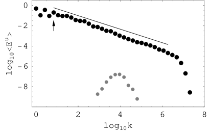
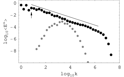
(a)	(b)
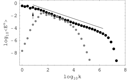
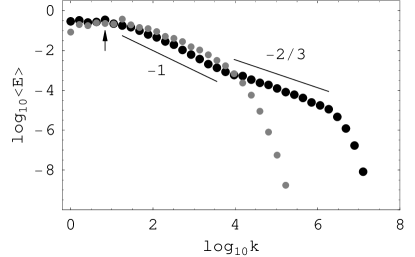
(c)	(d)

Figure 3: Kinetic (black dots) and magnetic (gray dots) spectra at four successive times (from (a) to (d)) for $n_{f}=4$, $\nu=10^{-9}$ and $\eta=10^{-6}$. See also the movie energy1.mpg in which $\log_{10}E^{U}(n)$ and $\log_{10}E^{B}(n)$ are plotted versus $\log_{10}k$ with respectively red and blue dots.

In Fig. 3 we show the kinetic and magnetic spectrum at four successive times for again $\nu=10^{-9}$ and $\eta=10^{-6}$ ($\mathrm{Pm}=10^{-3}$). Each snapshot corresponds to an average over a not so large amount of time which explains why at early time the kinetic spectrum is not very smooth at large scales. In the early time, when the magnetic field is still not significant, the kinetic energy spectrum has a slope in $k^{-2/3}$ (corresponding to a Fourier spectrum in $k^{-5/3}$). Then, as $\mathrm{Rm}$ is much larger than the critical value of the dynamo instability, the magnetic energy starts to grow (Fig. 3a). We expect magnetic energy to be initially amplified by the eddies having the highest sharing rate, i.e. the smallest scale eddies. As $\mathrm{Pm}<1$, the smallest eddies available for dynamo action correspond to eddies at resistive scale. This is indeed what we find, as here, the resistive scale (defined as in section 2.3) corresponds to $\log_{10}k_{\eta}\sim 4.1$. We note that the Kolmogorov resistive scale given by $k_{\eta}\sim(\epsilon/\eta^{3})^{1/4}$ (see section 4.3) with $\eta=10^{-6}$, leads to a slightly higher value $\log_{10}k_{\eta}\sim 4.5$.

As $\mathrm{Rm}$ is sufficiently large, at subsequent times the magnetic energy reaches the level of kinetic energy (Fig. 3c). At that time the kinetic spectrum is not influenced yet by the nonlinear feedback of the magnetic field and is still in $k^{-2/3}$. Then the dynamical equilibrium between the magnetic and velocity fields settles down (Fig. 3d). A striking feature of this equilibrium is the change of slope (from -2/3 to $\sim$ -1) of the kinetic energy spectrum for $k\leq k_{\eta}$ while the magnetic spectrum is slightly above the kinetic spectrum. We also note that the viscous dissipation scale has increased (the right part of the kinetic spectrum drifting to the left). This probably comes from the fact that there is less energy to dissipate by viscosity than at earlier time because of the additional Joule dissipation.

When changing the value of $\mathrm{Pm}$ while keeping the same value of $\nu$ and calculating again the final statistically stationary state, we observe again (Fig. 4) a deviation of the kinetic energy slope from -2/3 to $\sim$ -1 whatever the value of $\mathrm{Pm}$.

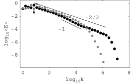
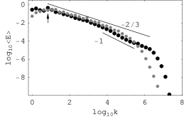
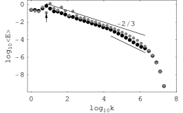
(a)	(b)	(c)

Figure 4: Kinetic (black dots) and magnetic (gray dots) spectra for $\nu=10^{-9}$ and for $\mathrm{Pm}=$ (a)$\;10^{-2}$, (b)$\;10^{-1}$, (c)$\;10^{0}$ and $\mathrm{Re}=$ (a)$\;6.5\;10^{9}$, (b)$\;4.4\;10^{9}$, (c)$\;4.4\;10^{9}$ . The forcing scale corresponds to $n_{f}=4$.

To understand better these spectra, we plotted several fluxes in Fig. 5, for $\nu=10^{-9}$ and $\mathrm{Pm}=10^{-3}$.

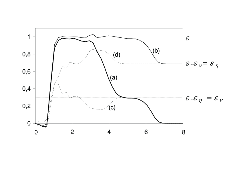
Figure 5: Spectral energy fluxes (a) $\Pi_{tot}(n)$,  (b) $\Pi_{U}(n)$,  (c) $\Pi_{U>}^{U<}(n)$,  (d) $\Pi_{U>}^{B<}(n)$ versus $\log_{10}k$ for $\nu=10^{-9}$ and $\mathrm{Pm}=10^{-3}$.

Looking at curve (a) which represents the total flux $\Pi_{tot}(n)$ versus $\log_{10}k$, one can distinguish three plateaus: the first one corresponds to scales larger than the resistive scale ($1\leq\log_{10}k\leq 3$), the second one for scales smaller than the resistive scale but larger than the viscous scale ($\log_{10}k\sim 5$), and the third one for scales smaller than the viscous scale ($\log_{10}k\geq 7$). The drop from the first to the second plateau corresponds to the ohmic dissipation rate $\epsilon_{\eta}=\sum_{j=0}^{N}D^{B}(j)$. The drop from the second to the third plateau corresponds to the viscous dissipation rate $\epsilon_{\nu}=\sum_{j=0}^{N}D^{U}(j)$. We clearly have $\epsilon=\epsilon_{\nu}+\epsilon_{\eta}$ as expected from (26) for $n=N$.

The curve (b) corresponds to $\Pi_{U}(n)$ versus $\log_{10}k$ with two plateaus, depending if the scale is larger or smaller than the viscous scale. The first plateau ($k\leq 6$) corresponds to $\Pi_{U}(n)\sim\epsilon$ and the second one ($k\geq 7$) to $\Pi_{U}(n)\sim\epsilon-\epsilon_{\nu}=\epsilon_{\eta}$. In particular, there is no clear change of $\Pi_{U}(n)$ just before the resistive scale that could explain the change of slope of the kinetic energy spectrum as previously pointed out.

Now let us have a look at curve (c). The transfer rate $\Pi_{U>}^{U<}(n)$ is responsible for the direct cascade of kinetic energy and would be constant leading to a Kolmogorov spectrum if the magnetic field was null (see Fig. 1). This would remain true for a non zero magnetic field only if the curve (c) was staying flat with $\Pi_{U>}^{U<}(n)=\epsilon_{\nu}$ for $2<\log_{10}k<5.5$. In that case the curve (d) would be flat as well with $\Pi_{U>}^{B<}(n)=\epsilon_{\eta}$ for $k>2$. Instead, there is a drop of $\Pi_{U>}^{U<}(n)$ compensated by a symmetric bump of $\Pi_{U>}^{B<}(n)$ for $2<\log_{10}k<4.5$. This drop of $\Pi_{U>}^{U<}(n)$ is consistent with a spectrum steeper than $k^{-2/3}$. Indeed, the bump of $\Pi_{U>}^{B<}(n)$ corresponds to some extra energy taken from $\epsilon$ and dissipated by Joule effect. Then there is less energy to be transferred through the kinetic energy cascade. The physical reason why this scenario happens for scales just larger than the resistive scale, however is still unclear.

For the parameters of Fig. 5 the Kolmogorov dissipation scales are given by $k_{\eta}=(\epsilon/\eta^{3})^{1/4}=10^{4.5}$ and $k_{\eta}=(\epsilon/\nu^{3})^{1/4}=10^{6.75}$ which correspond quantitatively well with the beginning of the second and third plateau of $\Pi_{tot}(n)$. This shows that the arguments leading to the Kolmogorov dissipation scales (see next section) are not affected by the change of spectra slopes observed in Fig. 4.

Finally for completeness, we produced three movies showing the time evolution of the spectra of the other quadratic quantities. In u-helicity.mpg, b-helicity.mpg and cross-helicity.mpg, $\log_{10}{\cal H}_{U}(n)$, $\log_{10}{\cal H}_{B}(n)$ and $\log_{10}{\cal H}_{C}(n)$ are plotted versus $\log_{10}k$ where the blue and red dots denote positive and negative signs.

4.3 Dissipation scales ratio

At the end of section 2.3 we have already explained how we identify the viscous and resistive scales $k_{\nu}$ and $k_{\eta}$, by comparing the turn over time to the respective dissipative times. In Fig. 6 we plot the ratio $k_{\nu}/k_{\eta}$ versus $\mathrm{Pm}\leq 1$ for different values of $\mathrm{Re}$. We find that $k_{\nu}/k_{\eta}\sim\mathrm{Pm}^{-3/4}$. To understand why, it is sufficient to say that between $k_{\eta}$ and $k_{\nu}$ the kinetic energy obeys a Kolmogorov spectrum $U(k)=\epsilon^{1/3}k^{-1/3}$ (see Fig. 4), leading to $\tau_{U}^{-1}=kU(k)=\epsilon^{1/3}k^{2/3}$. Comparing $\tau_{U}^{-1}$ with respectively $\tau_{\nu}^{-1}=\nu k^{2}$ and $\tau_{\eta}^{-1}=\eta k^{2}$ leads [47] to the dissipation scales $k_{\nu}\sim(\nu^{3}/\epsilon)^{-1/4}$ and $k_{\eta}\sim(\eta^{3}/\epsilon)^{-1/4}$. This in turn leads to a dissipation scales ratio in $\mathrm{Pm}^{-3/4}$.

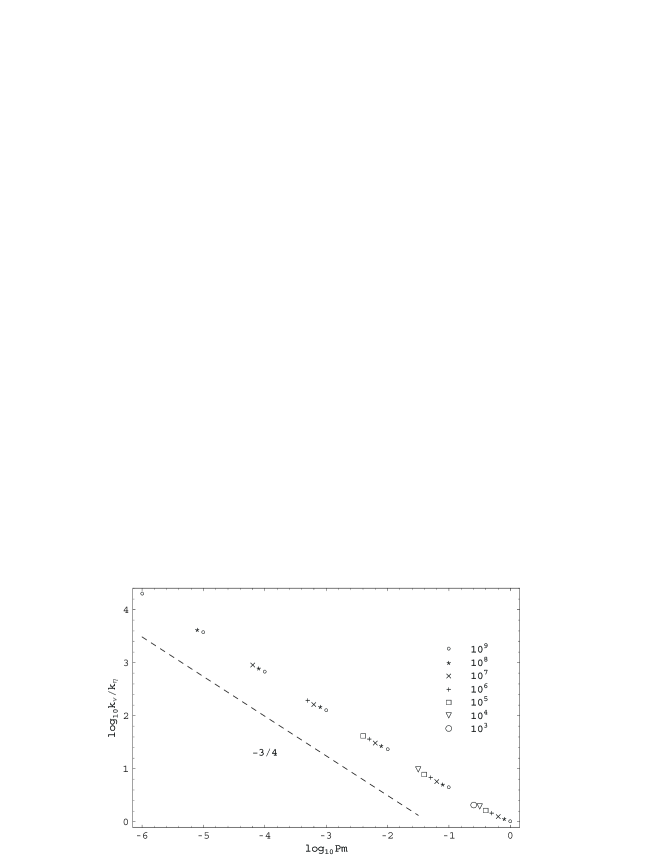
Figure 6: Ratio $k_{\nu}/k_{\eta}$ versus $\mathrm{Pm}$ for different values of $\nu^{-1}$ indicated in the legend. The straight line $k^{-3/4}$ is plotted (dashed line) for comparison.

4.4 Route to saturation

In this section we study the influence of $\mathrm{Pm}$ on the way the dynamo saturates. For that we calculate the ratio of magnetic to kinetic energy $E_{B}/E_{U}$, $E_{B}$ and $E_{U}$ being defined as in (12). In Fig. 7, $E_{B}/E_{U}$ is plotted versus $\mathrm{Rm}$ for three values of $\mathrm{Pm}$. We note that for $\mathrm{Rm}$ much larger than the critical value, the level of saturation $E_{B}/E_{U}$ may go beyond 1 for $\mathrm{Rm}\sim 10^{5}$. Such a super saturation state could be expected from the spectra of Fig. 4. At the threshold, the slope of $E_{B}/E_{U}$ versus $\mathrm{Rm}$ follows a turbulent scaling of the form $E_{B}/E_{U}\sim(\mathrm{Rm}-\mathrm{Rm}_{c})/\mathrm{Rm}_{c}^{2}$ as expected by Pétrélis and Fauve [49]. Indeed as in this case the threshold $\mathrm{Rm}_{c}$ does not vary very much with $\mathrm{Pm}$, the slopes at $\mathrm{Rm}=\mathrm{Rm}_{c}$ are similar. This is to contrast with the laminar scaling $E_{B}/E_{U}\sim\mathrm{Pm}(\mathrm{Rm}-\mathrm{Rm}_{c})/\mathrm{Rm}_{c}^{2}$ [49] which would lead to a quasi-horizontal slope for $\mathrm{Pm}=10^{-4}$.

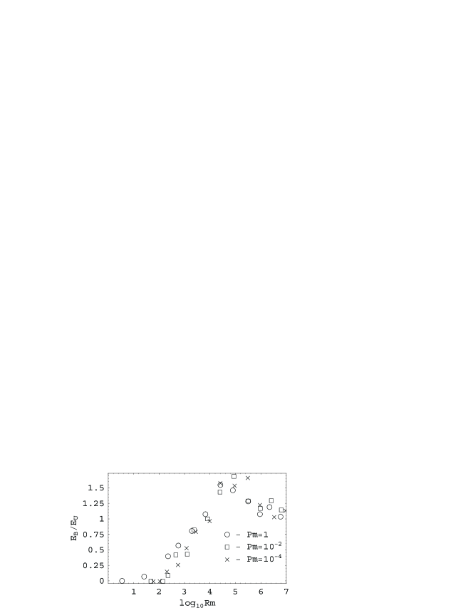
Figure 7: The energy ratio $E_{B}/E_{U}$ versus $\mathrm{Rm}$ for $n_{f}=4$ and three values of $\mathrm{Pm}$.

4.5 Dynamo threshold

In Fig. 8 the dynamo threshold $\mathrm{Rm}_{c}$ is plotted versus $\mathrm{Pm}^{-1}$ for $n_{f}=4$. For increasing values of $\mathrm{Pm}^{-1}$ up to $10^{3}$ the threshold first increases in accordance with previous direct numerical simulations [4, 5, 6, 7, 8, 9]. However, for values of $\mathrm{Pm}^{-1}$ larger than $10^{3}$ the threshold $\mathrm{Rm}_{c}$ is found to reach a plateau.

For each value of $\mathrm{Pm}$, the vertical bar around $\mathrm{Rm}_{c}$ corresponds to values of $\mathrm{Rm}$ for which the magnetic solution is erratic. In other words, below the bars there is no dynamo action and above the bars there is a well define statistically stationary magnetic solution. In between though we do not observe intermittency as in [50, 51], the dynamo is irregular, the mean magnetic energy increasing and decreasing versus time.

Figure 8: Dynamo threshold $\mathrm{Rm}_{c}$ versus $\mathrm{Pm}^{-1}$ for $n_{f}=4$.

4.6 Influence of a forcing scale smaller than the resistive dissipation scale

In Fig. 9, the kinetic and magnetic spectra are plotted for a forcing scale smaller than the resistive scale $k_{\eta}$. In that case the inertial range does not play a role in the magnetic generation and a kinetic spectra in $k^{-2/3}$ is recovered.

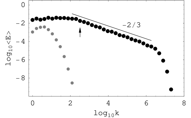
Figure 9: Kinetic (black dots) and magnetic (gray dots) stationary spectra for $\nu=10^{-9}$, $\mathrm{Pm}=10^{-7}$ and a forcing scale corresponding to $n_{f}=12$. See also the movie energy2.mpg in which $\log_{10}E^{U}(n)$ and $\log_{10}E^{B}(n)$ are plotted versus $\log_{10}k$ with respectively red and blue dots.

5 Discussion

In this paper we investigated the fully developed MHD turbulence at magnetic Prandtl number lower than unity, using a shell model of MHD turbulence with an appropriate forcing. The main results are:
1. For strong MHD turbulent dynamo states (large $\mathrm{Rm}$) we find kinetic and magnetic energy spectra close to the Kolmogorov spectrum $k^{-2/3}$ except at scales just larger than the resistive dissipation scale for which there is a weaker (stronger) slope of the kinetic (magnetic) spectrum. This corresponds to the work of the Lorentz forces which increases with $k$ up to $k=k_{\eta}$.
2. The evaluation of the viscous and resistive dissipation scales are consistent with Kolmogorov estimates leading to $k_{\nu}/k_{\eta}\sim\mathrm{Pm}^{-3/4}$.
3. At the dynamo threshold $\mathrm{Rm}_{c}$, the ratio of magnetic to kinetic energy scales like $E_{B}/E_{U}\sim(\mathrm{Rm}-\mathrm{Rm}_{c})/\mathrm{Rm}_{c}^{2}$, as predicted by a turbulent scaling [49].
4. At very low values of $\mathrm{Pm}$, the dynamo threshold $\mathrm{Rm}_{c}$ reaches a plateau.

Of course all these results rely on the assumption that the interactions between the different scales of motion and magnetic field are local interactions, each shell interacting with a few shells above and below. We believe that this should not make much difference as long as $\mathrm{Pm}$ is small, the Kolmogorov turbulence being governed by local interaction. In the other hand our results can not being tested against the Iroshnikov-Kraichnan $k^{-3/2}$ Fourier spectrum prediction [52] resulting from non local interactions between the flow and some large scale magnetic field which could result for example from dynamo action. By the way we believe that the $k^{-3/2}$ slope in FS98 is due to a lack of statistics as can be seen from the energy fluxes which are not flat and from the corresponding small range of scales. Adding some non local interaction with a large scale magnetic field in a local shell model, Biskamp [34] found a $k^{-3/2}$ slope, though taking only one such a non local interaction is somewhat artificial. Recently Verma [53] revisited the Iroshnikov-Kraichnan theory in which he shows that the large scale magnetic field becomes renormalized due to the nonlinear term, leading back to the Kolmogorov spectrum. This emphasizes the need for a complete nonlocal shell model in which any shell could interact with the others. This could be a good test against one theory or the other. Such a model would be also welcome for simulations at large $\mathrm{Pm}$. Indeed at large $\mathrm{Pm}$ we expect the more energetic scales of the flow, corresponding to scales close to the viscous scales, to interact directly with the smaller scales of the magnetic field. Our local shell model can not catch such features and this is why we did not show results at large $\mathrm{Pm}$ for they surely lack physical ground. A further issue that could be addressed by a nonlocal shell model could be to distinguish between a large scale field generated by a small scale velocity field resulting from non local interactions (developed in the mean field formalism) and a large scale field generated by an ”inverse cascade” as for example in Fig. 3 or in [54], resulting from local interactions.
Concerning our local model, we believe that the results presented in Fig. 8 showing that the dynamo threshold does not depend on $\mathrm{Pm}$ at low values of $\mathrm{Pm}$ would stay qualitatively the same if additional nonlocal interactions were included in the model. Indeed the dynamo threshold corresponds to the growth start of the magnetic field which is then still not significant. Therefore any non local interactions (e.g. Alfven sweeping effect) might not change the threshold.

6 Acknowledgments

Most of this work was done during a stay of R. S. at the LEGI, with a grant from the Université Joseph Fourier, Grenoble, France and completed during the visit of F.P. at the ICMM, Perm, Russia, supported by the ECO-NET program 10257QL. R.S. is also thankful for support from the BRHE program.

7 Appendix

For the pure hydrodynamic case ($B_{n}=0$), only the two first conditions (8) and (9) are necessary to derive the forcing equations. In that case the forcing set writes

$$f_{0} = \frac{\lambda\varepsilon}{(\lambda+1)u_{0}\cos(\phi_{0}-\omega_{0})}$$ (30)

$$f_{1} = \frac{\varepsilon}{(\lambda+1)u_{1}\cos(\phi_{1}-\omega_{1})}$$ (31)

$$f_{2} = 0,$$ (32)

while for the full MHD case the forcing set is derived from the three conditions (8), (9) and (10)

$$\frac{A}{\varepsilon}(1+\lambda)f_{0} = \lambda b_{2}u_{1}\cos(\theta_{2}-\phi_{2})\,\cos(\phi_{1}-\omega_{1})$$ (33)

$$+ \lambda^{2}b_{1}u_{2}\cos(\theta_{1}-\phi_{1})\,\cos(\phi_{2}-\omega_{2})$$

$$\frac{A}{\varepsilon}(1+\lambda)f_{1} = b_{2}u_{0}\cos(\theta_{2}-\phi_{2})\cos(\phi_{0}-\omega_{0})$$ (34)

$$- \lambda^{2}b_{0}u_{2}\cos(\theta_{0}-\phi_{0})\cos(\phi_{2}-\omega_{2})$$

$$\frac{A}{\varepsilon}(1+\lambda)f_{2} = -b_{1}u_{0}\cos(\theta_{1}-\phi_{1})\cos(\phi_{0}-\omega_{0})$$ (35)

$$- \lambda b_{0}u_{1}\cos(\theta_{0}-\phi_{0})\cos(\phi_{1}-\omega_{1})$$

where

$$A =b_{2}u_{0}u_{1}\cos(\theta_{2}-\phi_{2})\cos(\phi_{0}-\omega_{0})\cos(\phi_{1}-\omega_{1})$$ (36)

$$+ (\lambda-1)b_{1}u_{0}u_{2}\cos(\theta_{1}-\phi_{1})\cos(\phi_{0}-\omega_{0})\cos(\phi_{2}-\omega_{2})$$

$$- \lambda b_{0}u_{1}u_{2}\cos(\theta_{0}-\phi_{0})\cos(\phi_{1}-\omega_{1})\cos(\phi_{2}-\omega_{2})$$

and where $u_{j}$ and $\omega_{j}$ (resp. $b_{j}$ and $\theta_{j}$) are the complex modulus and argument of $U_{n_{f}+j}$ (resp. $B_{n_{f}+j}$).

References

- [1] G. Rüdiger and R. Hollerbach, 2004, The magnetic Universe, Wiley-VCH.
- [2] A.A. Schekochihin, S.C. Cowley and S.F. Taylor 2004, Simulations of the small-scale turbulent dynamo, ApJ 612 276.
- [3] Y. Ponty, P.D. Mininni, A. Pouquet, H. Politano, D.C. Montgomery and J.-F. Pinton, 2005, Numerical study of dynamo action at low magnetic Prandtl numbers, Phys. Rev. Lett. 94 164502.
- [4] A. Nordlund, A. Brandenburg, R.L. Jennings, M. Rieutord, J. Ruokolainen, R. Stein and I. Tuominen, 1992, Dynamo action in stratified convection with overshoot, Astrophys. J., 392 647.
- [5] A. Brandenburg, R.L. Jennings, A. Nordlund, M. Rieutord, R. Stein and I. Tuominen, Magnetic structures in a dynamo simulation, 1996, J. Fluid Mech., 306 325.
- [6] C. Nore, M.E. Brachet, H. Politano and A. Pouquet, 1997, Dynamo action in the Taylor–Green vortex near threshold, Phys. Plasmas, 4 1.
- [7] U. Christensen, P. Olson and G.A. Glatzmaier, 1999, Numerical modeling of the geodynamo: a systematic parameter study, Geophys. J. Int., 138 393.
- [8] T.A. Yousef, A. Brandenburg and G. Rüdiger, 2003, Turbulent magnetic Prandtl number and magnetic diffusivity quenching from simulations, Astron. Astrophys., 411 321.
- [9] A.A. Schekochihin, S.C. Cowley, J.L. Maron and J.C. McWilliams, 2004, Critical magnetic Prandtl number for small-scale dynamo Phys. Rev. Lett., 92 54502.
- [10] I. Rogachevskii and N. Kleeorin, 2004, Nonlinear theory of a “shear-current” effect and mean-field magnetic dynamos Phys. Rev. E, 70 046310.
- [11] A. Gailitis, O. Lielausis, S. Dementiev, E. Platacis, A. Cifersons, G. Gerbeth, Th. Gundrum, F. Stefani, M. Christen, H. Hänel and G. Will, 2000, Detection of a Flow Induced Magnetic Field Eigenmode in the Riga Dynamo Facility, Phys. Rev. Lett., 84 4365.
- [12] A. Gailitis, O. Lielausis, E. Platacis, S. Dementiev, A. Cifersons, G. Gerbeth, Th. Gundrum, F. Stefani, M. Christen and G. Will, 2001, Magnetic Field Saturation in the Riga Dynamo Experiment, Phys. Rev. Lett., 86 3024.
- [13] R. Stieglitz and U. Müller, 2001, Experimental demonstration of a homogeneous two-scale dynamo, Phys. Fluids, 13 561.
- [14] U. Müller, R. Stieglitz and S. Horanyi, 2004, A two-scale hydromagnetic dynamo experiment, J. Fluid Mech., 498 31-71.
- [15] M. Bourgoin, L. Marié, F. Pétrélis, C. Gasquet, A. Guigon, J.-B. Luciani, M. Moulin, F. Namer, J. Burgete, A. Chiffaudel, F. Daviaud, S. Fauve, P. Odier and J.-F. Pinton, 2002, Magnetohydrodynamics measurements in the von Karman sodium experiment, Phys. Fluids, 14 3046-3058.
- [16] F. Ravelet, A. Chiffaudel, F. Daviaud and J. Léorat, 2005, Towards an experimental von Karman dynamo: numerical studies for an optimized design, Phys. Fluids, submitted.
- [17] P. Frick, V. Noskov, S. Denisov, S. Khripchenko, D. Sokoloff, R. Stepanov, A. Sukhanovsky, 2002, Non-stationary screw flow in a toroidal channel: way to a laboratory dynamo experiment, Magnetohydrodynamics, 38, 143-162
- [18] C. Normand, 2003, Ponomarenko dynamo with time-periodic flow, Phys. Fluids, 15 1606-1611.
- [19] N. Leprovost, 2004, Influence des petites chelles sur la dynamique grande chelle en turbulence hydro et magn tohydrodynamique, PhD thesis, Paris 6.
- [20] R. Stepanov and K.-H. Rädler, 2004, The dynamo in a turbulent screw flow, Advances in Turbulence X (Proceedings of the Tenth European Turbulence Conference, 789-792
- [21] J.-P. Laval, P. Blaineau N. Leprovost, B. Dubrulle and F. Daviaud 2006, Influence of turbulence on the dynamo threshold, submitted.
- [22] G.O. Roberts, 1972, Spatially periodic dynamos, Phil. Trans. R. Soc. Lond. A, 271 411.
- [23] Y. B. Ponomarenko, 1973, Theory of the hydromagnetic generator, J. Appl. Mech. Tech. Phys., 14 775-778.
- [24] M.L. Dudley and R.W. James, 1989, Time-dependent kinematic dynamos with stationary flows, Proc. R. Soc. Lond. A, 425 407-429.
- [25] R.M. Kulsrud and S.W. Anderson, 1992, Time-dependent kinematic dynamos with stationary flows, Astrophys. J., 396 606.
- [26] S. Boldyrev and F. Cattaneo, 2004, Magnetic-field generation in Kolmogorov turbulence, Phys. Rev. Lett., 92 144501.
- [27] J. Léorat, A. Pouquet and U. Frisch, 1981, Fully developed MHD turbulence near critical magnetic Reynolds number, J. Fluid Mech., 104 419-443.
- [28] P. Frick and D. Sokoloff, 1998, Cascade and dynamo action in a shell model of magnetohydrodynamic turbulence, Phys. Rev. E, 57 4155.
- [29] P. G. Frick, 1983, Two-dimensional MHD turbulence. Hierarchical Model, Magn. Gidrodin., 1 60 [Magnetohydrodynamics 20, 262 (1984)].
- [30] C. Gloaguen, J. Léorat, A. Pouquet and R. Grappin, 1985, A scalar model for MHD turbulence, Physica D, 51 154.
- [31] R. Grappin, J. Léorat and A. Pouquet, 1986, J. Phys. (France), 47 1127.
- [32] V. Carbone and P. Veltri, 1990, Geophys. Astrophys. Fluid Dynam., 52 153.
- [33] V. Carbone, 1994, Scale similarity of the velocity structure functions in fully developed magnetohydrodynamic turbulence, Phys. Rev. E, 50 671 [Eurphys. Lett. 27, 581 (1994)].
- [34] D. Biskamp, 1994, Cascade models for magnetohydrodynamic turbulence, Phys. Rev. E, 50 2702.
- [35] A. Brandenburg and K. Enquist and P. Olesen, 1996, Large-scale magnetic field from hydromagnetic turbulence in the very early universe, Phys. Rev. D, 54 1291.
- [36] E.B. Gledzer, 1973, System of hydrodynamic type admitting two quadratic integrals of motion, Dokl. Akad. Nauk. SSSR, 209 1046 [Sov. Phys. Dokl. 18, 216 (1973)].
- [37] M. Yamada and K. Ohkitani, 1987, Lyapunov spectrum of a chaotic model of three-dimensional turbulence, J. Phys. Soc. Jpn., 56 4210.
- [38] U. Frisch, 1995, Turbulence, the legacy of A.N. Kolmogorov, (Cambridge University Press, Cambridge).
- [39] L. Biferale, 2003, Shell model of energy cascade in turbulence, Annu. Rev. Fluid Mech., 35 441-468.
- [40] Ya. B. Zeldovich, 1956, The magnetic field in the two-dimensional motion of a conducting turbulent fluid, Zh. Eksp. Teor. Fiz., 31 154 [Sov. Phys. JETP 4, 460 (1957)].
- [41] P. Giulani and V. Carbone, 1998, A note on shell models for MHD turbulence, Europhys. Lett., 43 527-532.
- [42] S.A. Lozhkin, D.D. Sokolov and P.G. Frik, 1999, Magnetic Prandtl number and the small-scale MHD dynamo, Astron. Rep., 43 753-758.
- [43] G.K. Batchelor, 1950, On the spontaneous magnetic field in a conducting liquid in turbulent motion, Proc. R. Soc. London A, 201 405.
- [44] V. L’vov, E. Podivilov, A. Pomyalov, I. Procaccia and D. Vandembroucq, 1998, Improved shell model of turbulence, Phys. Rev. E, 58 1811.
- [45] L. Kadanoff, D. Lohse, J. Wang and R. Benzi, 1995, Scaling and dissipation in the GOY shell model, Phys. Fluids, 7 617-29.
- [46] M. K. Verma, 2004, Statistical theory of magnetohydrodynamic turbulence: recent results, Phys. Reports, 401 229-380.
- [47] R.H. Kraichnan and S. Nagarajan, 1967, Growth of turbulent magnetic field Phys. Fluids, 10 859.
- [48] W. Dobler, N. Haugen, T. Yousef and A. Brandenburg 2004, Bottleneck effect in three-dimensional turbulence simulations, Phys. Rev. E, 68 026304.
- [49] F. Pétrélis and S. Fauve, 2001, Saturation of the magnetic field above the dynamo threshold, Eur. Phys. J. B, 22 273-276.
- [50] N. Leprovost and B. Dubrulle, 2005, The turbulent dynamo as an instability in a noisy medium, Eur. Phys. J. B, 44 395-400.
- [51] N. Leprovost, B. Dubrulle and F. Plunian 2006, Instability in presence of noise: the example of homopolar dynamo, submitted to Magnetohydrodynamics.
- [52] D. Biskamp 2003, Magnetohydrodynamic Turbulence, (Cambridge University Press, Cambridge)).
- [53] M. K. Verma, 1999, Mean magnetic field renormalization and Kolmogorov’s energy spectrum in magnetohydrodynamic turbulence, Phys. Plasmas, 6 1455-1460.
- [54] A. Pouquet, U. Frisch and J. Léorat, 1976, Strong MHD helical turbulence and the non linear dynamo effect, J. Fluid Mech., 77 321-354.