Accurate numerical solutions of the time-dependent Schrödinger equation

Abstract

We present a generalization of the often-used Crank-Nicolson (CN) method of obtaining numerical solutions of the time-dependent Schrödinger equation. The generalization yields numerical solutions accurate to order $(\Delta x)^{2r-1}$ in space and $(\Delta t)^{2M}$ in time for any positive integers $r$ and $M$, while CN employ $r=M=1$. We note dramatic improvement in the attainable precision (circa 10 or greater orders of magnitude) along with several orders of magnitude reduction of computational time. The improved method is shown to lead to feasible studies of coherent-state oscillations with additional short-range interactions, wavepacket scattering, and long-time studies of decaying systems.

I Introduction

Whereas there are a number of examples of exact analytic solutions of time-independent problems in quantum mechanics, such solutions of time-dependent problems are few. The analytic solutions of both types that do exist tend to provide approximate models to actual physical systems. No doubt such solutions are instructive for gaining insight into the behavior of the physical systems that they describe. Nevertheless because the models themselves are often approximations and because one wishes to describe real systems as precisely as possible, one also relies on accurate numerical methods.

The time-dependence of nonrelativistic quantum systems, which is the focus of this paper, has become important in diverse areas of atomic and subatomic physics. Examples of these include the study of nuclear processes such as the decay of unstable nuclei and associated phenomena like atomic ionization van Dijk et al. (1999); Kataoka et al. (2000) and bremsstrahlung Bertulani et al. (1999); van Dijk and Nogami (2003a); Ş. Mişicu et al. (2001), the study of fundamental processes necessary for quantum computing Cheon et al. (2004), the study of mesoscopic physics or nanophysics devices Veenstra et al. (2006), and the motion of atoms in a trap. A reliable and accurate numerical determination of the time-dependent wave function such as we discuss in this paper will no doubt be necessary and/or helpful in making advances in the understanding of a variety of quantum processes.

In this paper we consider the numerical solution of the time-dependent nonrelativistic Schrödinger equation. Much has been learned about basic scattering processes from the numerically generated solutions of traveling wavepackets as they pass through a potential region Goldberg et al. (1967), as well as the time-evolution of unstable quantum processes Winter (1961). However, the methods used in the past, and still employed currently, are limited in that the solutions often degrade after a certain time interval, so that they reduce to noise. Furthermore for processes in which the wave function spreads or travels away from the source one often requires such a large number of space steps that the computation becomes prohibitive.

The goal of this study is to improve the existing standard approach by allowing for relatively large step sizes both in time and in space and thus to reduce the number of basic arithmetical calculations while obtaining more accurate solutions. We have been able to make significant improvement to one conventional approach, viz., the Crank-Nicolson (CN) implicit integration scheme for the time-dependent Schrödinger equation. Many years ago the CN approach was shown to be successful in the study of wavepacket scattering in one dimension by Goldberg et al. Goldberg et al. (1967). In recent years the CN method continues to be employed for its space- and/or time-development algorithm to study various time-dependent problems. See, for example, Refs. Press et al. (1992); Patriarca (1994); Qian et al. (2006); Vyas et al. (2006). The attractive aspect of this method is that the solution is constrained to be unitary at every time step. It is this constraint that makes the solution stable regardless of time- or space-step size. Although the evolution of the solution is unitary, the wave function is not correct if the step sizes are too large. The error is of ${\cal O}({(\Delta x)^{2},(\Delta t)^{3}})$, where $\Delta x$ and $\Delta t$ are the spatial and temporal step size, respectively.

The method was successfully generalized to two dimensional scattering by Galbraith et al. Galbraith et al. (1984) and, more recently, to multichannel scattering van Dijk et al. (2003). Furthermore alternative methods which are fast computationally were introduced by Kosloff and Kosloff Kosloff and Kosloff (1983). These involve the fast Fourier transform of the kinetic energy operator of the Schrödinger equation. Variants of this method were discussed in Ref. Leforestier et al. (1991). Although this approach is fast and is able to handle large time intervals in one pass, it is not unitary and does require a large number of space intervals.

Improved CN algorithms have been discussed by a few authors. Mişucu et al. Ş. Mişicu et al. (2001) introduced a seven-point formula for the second-order spatial derivative with error of ${\cal O}((\Delta x)^{6})$ and an improved time-integration scheme with an error of ${\cal O}((\Delta t)^{5})$. They claim to obtain two orders of magnitude improvement in the time advance. Moyer Moyer (2004) uses a Numerov scheme for the spatial integration method with error of ${\cal O}((\Delta x)^{6})$ but has a one-stage time evolution giving the CN precision in time, i.e., with an error of ${\cal O}((\Delta t)^{3})$. Moyer also introduces transparent boundary conditions for unconfined systems. We have found these very useful for making long-time or large-space problems tractable Veenstra et al. (2006), but we will not discuss such boundary conditions further in this paper. Puzynin et al. Puzynin et al. (1999, 2000) indicate how to generalize the time development to higher order, but do not discuss spatial integration.

In this paper we present a generalization of the often-used CN method of obtaining numerical solutions of the time-dependent Schrödinger equation. The generalization yields numerical solutions accurate to order $(\Delta x)^{2r-1}$ in space and $(\Delta t)^{2M}$ in time for any positive integers $r$ and $M$, while CN employ $r=M=1$. By appropriate choice of $r$ and $M$ the improvement can be of such a nature that hitherto computationally unfeasible problems become doable, and solutions with low to modest precision can now be obtained extremely accurately.

In the following we consider the generalization of spatial integration in Sec. II and the generalization of the time integration in Sec. III. In Sec. IV we discuss errors and a way of dealing with a particular type of boundary condition. We study specific examples to illustrate the improvement of the generalizations over the standard CN procedure in Sec. V. Some general observations and conclusions are made in Sec. VI.

II Spatial integration

We describe a general procedure for solving the one-dimensional time-dependent Schrödinger equation

$$\left(i\hbar\frac{\partial~{}}{\partial t}-H\right)\psi(x,t)=0,\hskip 14.45377pt\psi(x,t_{0})=\phi(x),$$ (2.1)

where

$$H=-\frac{\hbar^{2}}{2m}\frac{\partial^{2}~{}}{\partial x^{2}}+V(x),$$ (2.2)

and $\phi(x)$ is a given wave function at initial time $t_{0}$. In this section we use the standard time-advance procedure of the CN method, but generalize the spatial integration. In Sec. III we generalize the time-evolution procedure.

The time evolution of the system can be expressed in terms of an operator acting on the wave function at time $t$ which gives the wave function at a later time $t+\Delta t$ according to the equation

$$\psi(x,t+\Delta t)=e^{\textstyle-iH\Delta t/\hbar}\psi(x,t).$$ (2.3)

The time-evolution operator $e^{\textstyle-iH\Delta t/\hbar}$ can be expanded to give a unitary approximation of the operator by setting

$$e^{\textstyle-iH\Delta t/\hbar}=\frac{1-{1\over 2}{iH\Delta t/\hbar}}{1+{1\over 2}{iH\Delta t/\hbar}}+{\cal O}((\Delta t)^{3}).$$ (2.4)

Inserting the approximate form of the operator into Eq. (2.3), we obtain the equation

$$\left(1+{1\over 2}iH\Delta t/\hbar\right)\psi(x,t+\Delta t)=\left(1-{1\over 2}iH\Delta t/\hbar\right)\psi(x,t),$$ (2.5)

with an error of ${\cal O}((\Delta t)^{3})$. Here we focus on the second-order spatial derivative in $H$ of Eq. (2.2) and leave improvements with respect to the time derivative to Sec. III. We generalize the usual three-point formula and the seven-point formula of Mişicu et al. Ş. Mişicu et al. (2001), for the second-order derivative to a $(2r+1)$-point formula. Such a formula has the form

$$y^{\prime\prime}(x)\equiv y^{(2)}=\frac{1}{h^{2}}\sum_{k=-r}^{k=r}c_{k}^{(r)}\,y(x+kh)+{\cal O}(h^{2r}),$$ (2.6)

where $c_{k}^{(r)}$ are real constants. To obtain the coefficients $c_{k}^{(r)}$ we make expansions

$$y(x+kh) = y(x)+(kh)y^{(1)}(x)+\frac{1}{2!}(kh)^{2}y^{(2)}(x)+\cdots+\frac{1}{(2r+1)!}(kh)^{2r+1}y^{(2r+1)}(x)+{\cal O}(h^{2r+2})$$

$$y(x-kh) = y(x)-(kh)y^{(1)}(x)+\frac{1}{2!}(kh)^{2}y^{(2)}(x)-\cdots+\frac{(-1)^{2r+1}}{(2r+1)!}(kh)^{2r+1}y^{(2r+1)}(x)+{\cal O}(h^{2r+2}),$$

for $k=1,2,\dots,r$; $y^{(i)}$ denotes the $i$th derivative with respect to $x$. When we add the two equations, the terms with odd-order derivatives cancel, resulting in the equation

$$2\frac{(kh)^{2}}{2!}y^{(2)}(x)+2\frac{(kh)^{4}}{4!}y^{(4)}(x)+\cdots+2\frac{(kh)^{2r}}{(2r)!}y^{(2r)}(x)=y(x+kh)+y(x-kh)-2y(x)+{\cal O}(h^{2r+2}).$$ (2.7)

Thus we obtain the system of $r$ equations in $r$ unknowns, i.e., $y^{(2k)}(x)$ for $k=1,\dots,r$,

$$2\frac{(h)^{2}}{2!}y^{(2)}(x)+2\frac{(h)^{4}}{4!}y^{(4)}(x)+\cdots+2\frac{(h)^{2r}}{(2r)!}y^{(2r)}(x) = y(x+h)+y(x-h)-2y(x)$$

$$2\frac{(2h)^{2}}{2!}y^{(2)}(x)+2\frac{(2h)^{4}}{4!}y^{(4)}(x)+\cdots+2\frac{(2h)^{2r}}{(2r)!}y^{(2r)}(x) = y(x+2h)+y(x-2h)-2y(x)$$

$$\vdots\hskip 144.54pt$$

$$2\frac{(rh)^{2}}{2!}y^{(2)}(x)+2\frac{(rh)^{4}}{4!}y^{(4)}(x)+\cdots+2\frac{(rh)^{2r}}{(2r)!}y^{(2r)}(x) = y(x+rh)+y(x-rh)-2y(x).$$ (2.8)

We solve these equations to obtain $y^{(2)}(x)$. It is evident from the terms on the right side of Eqs. (2.8) that $y^{(2)}(x)$ has the form of Eq. (2.6) and the coefficients $c_{k}^{(r)}$ can be identified. Because the equations (2.8) are invariant under the change of $h$ to $-h$, the coefficients satisfy the relation $c_{-k}^{(r)}=c_{k}^{(r)}$ for $k=1,2,\dots,r$. For example, the first seven sets of coefficients (up to the fifteen-point formula) are given in Table 1.

$r$	$k=0$	$1$	$2$	$3$	$4$	$5$	$6$	$7$
1	$-2$	1
2	$-\frac{5}{2}$	$\frac{4}{3}$	$-\frac{1}{12}$
3	$-\frac{49}{18}$	$\frac{3}{2}$	$-\frac{3}{20}$	$\frac{1}{90}$
4	$-\frac{205}{72}$	$\frac{8}{5}$	$-\frac{1}{5}$	$\frac{8}{315}$	$-\frac{1}{560}$
5	$-\frac{5269}{1800}$	$\frac{5}{3}$	$-\frac{5}{21}$	$\frac{5}{126}$	$-\frac{5}{1008}$	$\frac{1}{3150}$
6	$-\frac{5369}{1800}$	$\frac{12}{7}$	$-\frac{15}{56}$	$\frac{10}{189}$	$-\frac{1}{112}$	$\frac{2}{1925}$	$-\frac{1}{16632}$
7	$-\frac{266681}{88200}$	$\frac{7}{4}$	$-\frac{7}{24}$	$\frac{7}{108}$	$-\frac{7}{528}$	$\frac{7}{3300}$	$-\frac{7}{30888}$	$\frac{1}{84084}$

Table 1: The coefficients $c_{k}^{(r)}$ up to $r=7$.

Let us partition the range of $x$ and $t$ values so that $x_{j}=x_{0}+j\Delta x$, $j=0,1,\dots,J$ and $t_{n}=t_{0}+n\Delta t$, $n=0,1,\dots,N$. The numerical approximation of the wave function at a mesh point in space and time is denoted as $\psi_{j,n}\approx\psi(x_{j},t_{n})$ and we set $V_{j}=V(x_{j})$. Using expression (2.6) in Eq. (2.5), we obtain

$${\displaystyle\psi_{j,n+1}-\frac{i\hbar\Delta t}{4m(\Delta x)^{2}}\left[\sum_{k=-r}^{k=r}c_{k}^{(r)}\psi_{j+k,n+1}\right]+\frac{i\Delta t}{2\hbar}V_{j}\psi_{j,n+1}}$$

$$\mbox{~{}}{\displaystyle=\psi_{j,n}+\frac{i\hbar\Delta t}{4m(\Delta x)^{2}}\left[\sum_{k=-r}^{k=r}c_{k}^{(r)}\psi_{j+k,n}\right]-\frac{i\Delta t}{2\hbar}V_{j}\psi_{j,n}},$$ (2.9)

for $j=0$ to $J$. The indices in the sums may go out of range, so we set $\psi_{j,n}=0$ when $j<0$ and $j>J$. Define

$$b\equiv\frac{i\hbar\Delta t}{2m(\Delta x)^{2}},\ \ z_{1}^{(1)}\equiv-2\ \mbox{\rm~{}and~{}}\ a_{k}^{(r)}\equiv\frac{b}{z_{1}^{(1)}}c_{k}^{(r)},$$ (2.10)

and subsequently

$$d_{j}\equiv 1+a_{0}^{(r)}-\frac{i\Delta t/\hbar}{z_{1}^{(1)}}V_{j},\ \ j=0,1,\dots,J.$$ (2.11)

The notation includes $z_{1}^{(1)}$ which is consistent with that used in the generalization of the time dependence of the wave function discussed in the next section.

The solution $\psi_{j,n+1}$ is obtained by solving the system of linear equations

$$A\Psi_{n+1}=A^{*}\Psi_{n},$$ (2.12)

where the matrix $A$ is the $(2r+1)$-diagonal matrix

$$A=\left(\begin{array}[]{cccccccccc}d_{0}&a_{1}&a_{2}&\cdots&a_{r}&0\\ a_{1}&d_{1}&a_{1}&\cdots&a_{r-1}&a_{r}\\ a_{2}&a_{1}&d_{2}&\cdots&a_{r-2}&a_{r-1}\\ \vdots&\vdots&\vdots&&\vdots&\vdots\\ a_{r}&a_{r-1}&a_{r-2}&\cdots&d_{r}&a_{1}\\ 0&a_{r}&a_{r-1}&\cdots&a_{1}&d_{r+1}\\ &&&&&&\ddots\\ &&&&&&&&d_{J-1}&a_{1}\\ &&&&&&&&a_{1}&d_{J}\end{array}\right),$$ (2.13)

where the superscript $\mbox{}^{(r)}$ of the $a_{k}$ is assumed. The matrix $A^{*}$ is the complex conjugate of matrix $A$. The wave function at $t_{n+1}$, i.e., $\Psi_{n+1}$, is a column vector consisting of the $\psi_{j,n+1}$ as components, and can be determined if $\Psi_{n}$ is known. The matrix equation (2.12) can be solved using standard techniques.

III Time advance

In this section we extend the work of Puzynin et al. Puzynin et al. (1999, 2000). The basic idea is to replace the exponential operator $\exp(-iH\Delta t)$ by the diagonal Padé approximant. The $[M/M]$ Padé approximant of the exponential function may be written as

$$f(z)=e^{\textstyle z}=\frac{a_{0}+a_{1}z+\cdots+a_{M}z^{M}}{b_{0}+b_{1}z+\cdots+b_{M}z^{M}}=\frac{\displaystyle\sum_{m=0}^{M}a_{m}z^{m}}{\displaystyle\sum_{m^{\prime}=0}^{M}b_{m^{\prime}}z^{m^{\prime}}},$$ (3.1)

where the $a_{m}$ and the $b_{m^{\prime}}$ are complex constants. It is evident that when $z=0$, $a_{0}/b_{0}=1$, which makes one of the coefficients arbitrary. By convention we take $b_{0}=1$ which immediately fixes $a_{0}=1$. There are $2M$ constants remaining, which can be found from the known coefficients of the series expansion of the exponential function, giving an error term in Eq. (3.1) ${\cal O}(z^{2M+1})$. The property of Padé approximants that can be used to advantage is that, if $f(z)$ is unitary, so is its diagonal Padé approximant Baker, Jr. and Graves-Morris (1981).

In general we solve for the coefficients $a_{m}$ and $b_{m^{\prime}}$ by multiplying Eq. (3.1) by the denominator so that

$$\left(\sum_{m^{\prime}=0}^{M}b_{m^{\prime}}z^{m^{\prime}}\right)\left(\sum_{i=0}^{\infty}c_{i}z^{i}\right)=\left(\sum_{m=0}^{M}a_{m}z^{m}\right),$$ (3.2)

where the $c_{i}$ are known since $e^{\displaystyle z}=\sum_{i=0}^{\infty}z^{i}/i!$. Multiplying out the sums on the left side of Eq. (3.2), and equating the coefficients of $z$ through $z^{2M}$ on both sides, we obtain $2M$ equations in $2M$ unknowns. The last $M$ of these equations contain no $a_{m}$ and hence can be solved for the $b_{m^{\prime}}$, which in turn can be inserted in the first $M$ equations to obtain the $a_{m}$. The numerator and the denominator of the diagonal Padé approximant of the exponential function have been studied extensively Baker, Jr. and Graves-Morris (1981). When each is factored it is found that the roots of the denominator are the negative complex conjugates of the roots of the numerator. Thus the $[M/M]$ Padé approximant of the exponential function leads to

$$e^{\textstyle z}=\prod_{s=1}^{M}\left(\frac{1-z/z_{s}^{(M)}}{1+z/\bar{z}_{s}^{(M)}}\right)+{\cal O}(z^{2M+1}),$$ (3.3)

where $z_{s}^{(M)},\ s=1,\dots,M$, are the roots of the numerator, and $\bar{z}^{(M)}_{s}$ is the complex conjugate of $z^{(M)}_{s}$. These roots can be found to a desired precision for virtually any value of $M$. We have found them to 17 digit precision for $M$ up to 20, a sample of which for $M=1$ to 5, each rounded to five decimal places, is given in Table 2.

$M$	$s=1$	$2$	$3$	$4$	$5$
1	$-2.00000+i0.00000$
2	$-3.00000+i1.73205$	$-3.00000-i1.73205$
3	$-4.64437+i0.00000$	$-3.67781-i3.50876$	$-3.67781+i3.50876$
4	$-4.20758+i5.31484$	$-5.79242+i1.73447$	$-5.79242-i1.73446$	$-4.20758-i5.31483$
5	$-4.64935+i7.14205$	$-6.70391+i3.48532$	$-7.29348+i0.00000$	$-6.70391-i3.48532$	$-4.64935-i7.14205$

Table 2: The roots $z_{s}^{(M)}$ of the numerator of the Padé approximant of the exponential function for $M$ from 1 to 5.

We use the Padé approximant to express the time evolution operator. Define the operator

$$K_{s}^{(M)}\equiv\frac{1-\frac{\textstyle iH\Delta t/\hbar}{\textstyle z_{s}^{(M)}}}{1+\frac{\textstyle iH\Delta t/\hbar}{\textstyle\bar{z}_{s}^{(M)}}},$$ (3.4)

so that

$$e^{\textstyle-iH\Delta t/\hbar}=\prod_{s=1}^{M}K_{s}^{(M)}+{\cal O}((\Delta t)^{2M+1}).$$ (3.5)

Since $\Psi_{n+1}=e^{\textstyle-iH\Delta t/\hbar}\Psi_{n}$, we write the relation

$$\Psi_{n+1}=\prod_{s=1}^{M}K_{s}^{(M)}\Psi_{n}.$$ (3.6)

Defining $\Psi_{n+s/M}\equiv K_{s}^{(M)}\Psi_{n+(s-1)/M}$, we can solve for $\Psi_{n+1}$ recursively, starting with

$$\Psi_{n+1/M}=K_{1}^{(M)}\Psi_{n}.$$ (3.7)

Assuming that $\Psi_{n}$ is known, we determine $\Psi_{n+1/M}$ from Eq. (3.7) which has a form similar to that of Eq. (2.5). We use therefore the same method of Sec. II to obtain $\Psi_{n+1/M}$. This is repeated to obtain in succession $\Psi_{n+2/M},\Psi_{n+3/M},\dots,\Psi_{n+(M-1)/M},\Psi_{n+1}$. Since the operators $K_{s}^{(M)}$ commute, they can be applied in any order.

IV Discussion of errors and boundary conditions

IV.1 Errors

In this section we discuss the errors as a function of the orders of the method, i.e., $r$ and $M$. Let us separate the truncation errors due to the integration over space and those due to integration over time. At a given time $t$ the spatial integration with the $r$th-order expansion yields a truncation error

$$e^{(r)}=C^{(r)}(\Delta x)^{2r},$$ (4.1)

where $C^{(r)}$ is assumed to be slowly varying with $r$. Actually $C^{(r)}=|\psi^{(2r)}(x^{*},t)|/(2r!)$ for some $x^{*}$ in the range of spatial integration, and thus is model dependent. If we specify an acceptable error, the step size $\Delta x$ can be adjusted to obtain that error. Since $\Delta x=(x_{0}-x_{J})/J$, an adjustment of $\Delta x$ is equivalent to a change in $J$. Recalling that $x_{0}-x_{J}$ is fixed, we obtain

$$\Delta x=\frac{x_{0}-x_{J}}{J}=\left(\frac{e^{(r)}}{C^{(r)}}\right)^{1/2r},$$ (4.2)

and

$$e^{(r)}\approx\frac{\rm constant}{J^{2r}}.$$ (4.3)

We have assumed that $C^{(r)}$ is approximately constant. The CPU time for the calculation is proportional to the number of basic computer operations in solving the matrix equation (2.12). This involves elementary row operations on $r-1$ rows in $J-1$ columns to bring the matrix to upper triangular form, plus $J$ back substitutions to obtain the solution. Hence

$$\mathrm{CPU~{}time}\propto\mathrm{\#~{}operations}\propto Jr\propto\frac{r}{(e^{(r)})^{1/2r}}.$$ (4.4)

This form gives a minimum (optimum) CPU time which occurs when

$$r\approx-\frac{\ln e^{(r)}}{2}.$$ (4.5)

For the time integration we assume a truncation error independent of $r$. For a given $r$ the error due to finite $\Delta t$ has a first term in the expansion

$$e^{(M)}=C^{(M)}(\Delta t)^{2M+1},$$ (4.6)

where again $C^{(M)}$ is assumed to be a slowly varying function of $M$. We note that the factor $1\over 2$ in the numerator and denominator of Eq. (2.4) is replaced by $1/z_{s}^{(M)}$ in each of the $M$ factors (3.4) of Eq. (3.5). As $M$ increases the average over different values of $s$ of $|z_{s}^{(M)}|$, which we denote as $z^{(M)}_{\mathrm{avge}}$, also increases. In fact $z^{(M)}_{\mathrm{avge}}$ is a linear function of $M$ as is seen in Fig. 1.

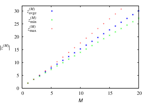
Figure 1: The average, the minimum and the maximum values of $\{|z_{s}^{(M)}|,s=1\dots M\}$, as a function of $M$.

The effective expansion parameter can be approximated by $2\Delta t/z^{(M)}_{\mathrm{avge}}$ rather than $\Delta t$ and hence is proportional to $\Delta t/M$. Thus we can replace the relation of Eq. (4.6) by

$$e^{(M)}\approx C^{(M)}(\Delta t/M)^{2M+1},$$ (4.7)

where the constant $C^{(M)}$ is appropriately adjusted. If we take the total time $t_{\mathrm{max}}=N\Delta t$ to be fixed, then

$$\mathrm{CPU~{}time}\propto\left(e^{(M)}\right)^{-\frac{\textstyle 1}{\textstyle 2M+1}}.$$ (4.8)

In Fig. 2 the curves of the (scaled) CPU times are plotted. Both curves clearly show the sharp decline when $r,M$ increases from 1 through 5 or larger. For increasing $M$ the CPU time continues to decline although the decrements become smaller at larger $M$. For increasing $r$ there is a minimum depending on the specified error and beyond the minimum the curve shows a slow increase with increasing $r$. Superimposed on the curves are the CPU times (as dots) of a model calculation (see Sec. V.1), in which the numerical and exact solutions can be compared. Clearly the theoretical trends, including the minimum as a function of $r$, occur in the computed example.

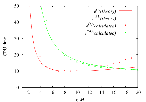
Figure 2: The normalized theoretical variation of the CPU time for a given error of $1.0\times 10^{-8}$. The calculated CPU times for the example of Sec. V.1 are shown as dots.

It should be noted that it “pays” to increase $M$ indefinitely, whereas there is an optimum value of $r$ which depends on the magnitude of $e^{(r)}$.

IV.2 Boundary conditions

Below Eq. (2.9) we indicate that we set $\psi_{j,n}=0$ when $j<0$ or $j>J$, or when $j$ goes out of range. These are appropriate boundary conditions when the wave function and its first $r+1$ derivatives are zero at the boundaries, since it was assumed in the derivation of the method that all these derivatives exist. If however that is not the case, for instance, at the boundary of an (in)finite square well or barrier where the second-order derivative does not exist, one must devise ways of incorporating the proper boundary conditions.

One case of importance, which we discuss in the third example (see Sec. V.3) of the paper, is the case of radial behavior of a partial wave when angular momentum decomposition has been done. In the $S$-wave case the wave function, defined only for nonnegative values of the radial coordinate, is zero at the origin but the first derivative is finite. Muller Muller (1999) discusses a related, but not identical, situation. He considers three-point formulas for the Coulomb potential which lead to a radial wave function which is zero when the radial variable $\rho=0$, but has first and second derivatives which are nonzero at $\rho=0$. His approach can be adapted to the $(2r+1)$-point formula of this work.

We treat this case by making the ansatz that the wave function behaves like an odd function about the origin and continues in the unphysical region of the negative radial variable. With this assumption we do not affect the behavior of the system at positive values of the radial variable, but all the required derivatives exist. Furthermore, the wave function at negative $j$ values can be combined with the ones with corresponding positive $j$ values, so that the space need not be enlarged but instead the first few matrix elements of the matrix $A$ can be changed to account for the boundary condition. This is achieved by replacing $A$ by $A^{\prime}=A-B$ in Eq. (2.13) where

$$B=\left(\begin{array}[]{cccccccccc}0&a_{1}&a_{2}&a_{3}&\cdots&a_{r-2}&a_{r-1}&a_{r}&0&\cdots\\ 0&a_{2}&a_{3}&a_{4}&\cdots&a_{r-1}&a_{r}&0&0&\cdots\\ 0&a_{3}&a_{4}&a_{5}&\cdots&a_{r}&0&0&0&\cdots\\ \vdots&\vdots&\vdots&\vdots&&\vdots&\vdots&\vdots&\vdots&\\ 0&a_{r-1}&a_{r}&0&\cdots&0&0&0&0&\cdots\\ 0&a_{r}&0&0&\cdots&0&0&0&0&\cdots\\ 0&0&0&0&\cdots&0&0&0&0&\cdots\\ \vdots&\vdots&\vdots&\vdots&&\vdots&\vdots&\vdots&\vdots&\\ \end{array}\right).$$ (4.9)

A hard-core type potential could be dealt with in the same way. Different forms of boundary conditions are more complicated to implement, but Ref. Muller (1999) suggests an approach to including such boundary conditions. For the purpose of the radial wave function of a nonsingular potential, the above approach is sufficient.

V Examples

We consider three systems to which this numerical method may be applied. The first two allow us to make a comparison with the exact solution and to test the precision of the numerical procedure. The third involves the time evolution of a quasi-stable quantum process.

V.1 Oscillation of a coherent wavepacket

The oscillation of a coherent state in the harmonic oscillator well is described in Ref. Schiff (1968). The time evolution of such states has been discussed recently in connection with the quantum abacus. (See Ref. Cheon et al. (2004).) In that case there is a point interaction at the center of the oscillator well. It is of interest to consider narrow but finite-range interactions to simulate more realistic physical systems. In order to test the robustness of the quantum gates one needs a very stable numerical procedure. We test the precision of the numerical procedure by investigating the case without the central interaction, so that the numerical results can be compared with the exact ones.

The time-dependent Schrödinger equation is

$$i\hbar\frac{\partial~{}}{\partial t}\psi(x,t)=\left(-\frac{\hbar^{2}}{2m}\frac{\partial^{2}~{}}{\partial x^{2}}+\frac{1}{2}Kx^{2}\right)\psi(x,t).$$ (5.1)

We consider the time evolution of the initially displaced ground-state wave function

$$\psi(x,0)=\frac{\alpha^{1/2}}{\pi^{1/4}}e^{-{1\over 2}\alpha^{2}(x-a)^{2}},$$ (5.2)

where $\alpha^{4}=mK/\hbar^{2}$, $\omega=\sqrt{K/m}$, and $a$ is the initial displacement. The closed expression for the time evolved wave function is

$$\psi_{\mathrm{exact}} = \frac{\alpha^{1/2}}{\pi^{1/4}}\exp\left[-\frac{1}{2}(\xi-\xi_{0}\cos{\omega t})^{2}\right.$$ (5.3)

$$\left.-i(\frac{1}{2}+\xi\xi_{0}\sin{\omega t}-\frac{1}{4}\xi_{0}^{2}\sin{2\omega t})\right],$$

where $\xi=\alpha x$ and $\xi_{0}=\alpha a$. We set $\hbar=m=1$, $\omega=0.2$, and $a=10$. We choose our space such that $x\in[x_{0},x_{J}]=[-40,40]$. The period of oscillation is then $T=10\pi$. We allow the coherent state to oscillate for eleven periods before comparing the numerical solution to the exact one. The error is calculated as $e_{2}$ using the formula Puzynin et al. (1999)

$$(e_{2})^{2}=\int_{x_{0}}^{x_{J}}\ dx\ |\psi(x,t_{1})-\psi_{\mathrm{exact}}(x,t_{1})|^{2},$$ (5.4)

where $t_{1}=11T$ for our example. The results including the relative CPU time  are displayed in Table 3.

$M$	$r$	$\Delta t$	$\Delta x$	$J$	$e_{2}$	CPU time
20	20	$\pi$	0.44444	180	$6.717\times 10^{-9}$	18.38
20	15	$\pi$	0.38095	210	$7.044\times 10^{-9}$	14.23
20	10	$\pi$	0.27586	290	$7.506\times 10^{-9}$	10.84
20	7	$\pi$	0.18182	440	$9.353\times 10^{-9}$	10.12
20	5	$\pi$	0.09877	810	$9.330\times 10^{-9}$	12.83
20	4	$\pi$	0.05755	1390	$9.871\times 10^{-9}$	18.61
20	3	$\pi$	0.03810	2100	$2.102\times 10^{-7}$	23.67
20	2	$\pi$	0.03810	2100	$1.624\times 10^{-4}$	18.42
20	1	$\pi$	0.03810	2100	$1.749\times 10^{-1}$	13.75
20	10	$\pi$	0.26667	300	$5.106\times 10^{-9}$	10.77
15	10	$\pi/1.5$	0.26667	300	$5.153\times 10^{-9}$	12.13
10	10	$\pi/3$	0.26667	300	$4.995\times 10^{-9}$	16.16
5	10	$\pi/15$	0.26667	300	$8.787\times 10^{-9}$	40.42
3	10	$\pi/150$	0.26667	300	$1.840\times 10^{-9}$	242.9
1	10	$\pi/3000$	0.26667	300	$5.046\times 10^{-4}$	1627

Table 3: Summary of computational time and errors incurred by using the numerical integration procedure when the initial wave function is the displaced ground state. The last column indicates a relative CPU run time. The upper half of the table gives the effects of changing the number of spatial steps; the lower half the effects of changing the number of time steps.

In the above tests we have tried to obtain a precision better than $10^{-8}$. While varying the number of steps for the spatial integration, we kept the number of time factors per time step constant at 20. Given that the total space is fixed and spans 80 units, we adjusted the number of spatial steps $J$ to give the required precision. We limited (arbitrarily) the maximum number of spatial steps to 2100. With $M=20$ the 15-point formula ($r=7$) is most efficient. When $r<4$ (less than 9-point formula), we were unable to reach the precision criterion because of the imposed limit on $J$. It is clear from the trend however that the efficiency is significantly less for the lower $r$ values. The 9-point formula is roughly half as efficient as the 15-point formula.

The effect of different order time formulas as seen in the lower part of Table 3 is even more dramatic. For the spatial integration we used the 21-point formula ($r=10$), and varied the time-order formula, i.e., $M$, from 20 to 1. We see at least two orders of magnitude improvement in computational speed as $M$ is increased over this range.

A comparison with the standard CN approach ($r=M=1$) is instructive. We considered the same system with $x_{0}=-25$ and $x_{J}=25$, $\Delta x=0.005$ and $\Delta t=0.5(\Delta x)^{2}$. The standard CN method yielded an error of $e_{2}=7.1\times 10^{-5}$ when $t=T/4$ which increased exponentially to $e_{2}=2.7\times 10^{-3}$ at $t=10T$. Whereas the CPU time in Table 3 is given in seconds, the CPU time required to complete this last calculation exceeded 24 hours.

The computed CPU times shown in Fig. 2 exceeded the “theoretic” values by increasing amounts as $r$ increased beyond 10. This can be attributed to the approximate nature of the error analysis in which the model dependence of $C^{(r)}$ (and $C^{(M)}$) was neglected. In this example a more elaborate analysis could be done since the wave function is known analytically. In practical situations where a numerical method is used the analytic wave function is usually not known and an estimate such as we have given here would be all that is available. The main point is that dramatic improvements result both theoretically and computationally when larger values of $r$ and $M$ are employed.

V.2 Propagation of a wavepacket

For this example we return to the work of Ref. Goldberg et al. (1967) and consider the main features of that analysis with a view of determining the improvement brought about by the generalizations of this paper. This problem was revisited by Moyer Moyer (2004) to illustrate the efficacy of the Numerov method and the use of transparent boundary conditions for the propagation of free-particle wavepackets. The authors of Ref. Goldberg et al. (1967) consider wavepackets impinging on a square barrier and study their behavior in time. We consider first free wavepacket propagation (without potential), and second the reflection and transmission of a wavepacket by a smooth potential.

Thus we first assume $V(x)=0$ and take as initial wave function

$$\psi(x,0)=(2\pi\sigma_{0}^{2})^{-1/4}e^{\textstyle ik_{0}(x-x_{0})}e^{\textstyle-(x-x_{0})^{2}/(2\sigma_{0})^{2}}.$$ (5.5)

(Note that our $\sigma_{0}$ is that of Ref. Goldberg et al. (1967) divided by $\sqrt{2}$.) The wave function at later time is given by

$$\mbox{~{}}\psi(x,t)=(2\pi\sigma_{0}^{2})^{-1/4}[1+i\hbar t/(2m\sigma_{0}^{2})]^{-1/2}\times$$

$$\exp{\left\{\frac{\textstyle-(x-x_{0})^{2}/(2\sigma_{0})^{2}+ik_{0}(x-x_{0})-i\hbar k_{0}^{2}t/(2m)}{\textstyle 1+i\hbar t/(2m\sigma_{0}^{2})}\right\}}.$$ (5.6)

We use parameters comparable to those of Ref. Goldberg et al. (1967). We set $\hbar=1$ and $m={1\over 2}$. The coordinate range we take is from $-0.5$ to 1.5 rather than from 0 to 1 since over the smaller space the normalization of the packet is not as precise as we require because the tails of the Gaussian are nonzero outside the (0,1) interval. We choose $\sigma_{0}=1/20$, $k_{0}=50\pi$, $\Delta t=2(\Delta x)^{2}$, and allow as much time as it takes the packet to travel from $x_{0}=0.25$ to around 0.75. For the final position the numerically calculated wave function is compared to the analytic one and $e_{2}$ is determined. In Table 4

$M$	$r$	$J$	$e_{2}$	CPU time
1	1	2000	$9.418\times 10^{-2}$	2.20
		4000	$2.189\times 10^{-2}$	18.04
		8000	$5.368\times 10^{-3}$	151.92
		16000	$1.336\times 10^{-3}$	1287.8
2	2	2000	$3.018\times 10^{-4}$	5.99
3	3	2000	$1.321\times 10^{-6}$	12.57
4	4	2000	$6.577\times 10^{-9}$	22.64
5	5	2000	$3.648\times 10^{-11}$	37.13
6	6	2000	$8.437\times 10^{-13}$	56.05
10	10	440	$3.606\times 10^{-9}$	2.12
20	20	260	$4.542\times 10^{-9}$	2.51

Table 4: Summary of computational parameters used to calculate the propagating free packet and compare it to the analytic wavepacket.

we list some of the computed results. We observe that the traditional CN method ($M=1$ and $r=1$) has a low precision and that using greater $J$ (smaller $\Delta x$) results in modest gain in precision. By using higher-order time formula one can make significant gain in precision (seven orders of magnitude) with no increase in computational time compared with that of Ref. Goldberg et al. (1967). (Compare the first row to the last two rows of Table 4.) Rows 5 through 9 of Table 4 illustrate the transition from less precise to more precise solutions. It is consistent with the finding of the authors of Ref. Ş. Mişicu et al. (2001) who use an $M=2$, $r=3$ method and obtain two orders of magnitude improvement of the results of Refs. Bertulani et al. (1999); van Dijk et al. (1999). The results are sensitive to surprisingly high orders of $\Delta x$ and $\Delta t$.

Another test using wavepacket scattering to show the efficacy of the higher-order approach is scattering from a potential. Rather than using the square barrier of Ref. Goldberg et al. (1967), we consider the repulsive Pöschl-Teller type potential Flügge (1974); Landau and Lifshitz (1977) of the form

$$V(x)=\frac{\hbar^{2}}{2m}\frac{\beta^{2}\lambda(\lambda-1)}{\cosh^{2}\beta x}.$$ (5.7)

Since this potential does not have discontinuities the improved CN method works well with it. The transmission and reflection coefficients are known analytically. We can also compute them by considering the wavepacket Eq. (5.5) incident on the potential. Over a sufficiently long time the wavepacket will have interacted with the potential and transmitted and reflected packets emerge and travel away from the potential region. At that point we can calculate the probabilities of the particle represented by the packet on the left and on the right of the potential; these probabilities correspond to the transmission and reflection coefficients provided the packet is sufficiently narrow in momentum space. This means that one needs an initial packet which is wide in coordinate space. In our calculation we choose $\beta=1$, $\lambda=2.5$, $m=1$, and $\sigma_{0}=10$. This gives a spread in the incident momentum-space wave packet of $\sigma_{k}=0.05$. The width in momentum space of the reflected and transmitted wavepackets also has this value. The domain of the $x$ coordinates is from $-300$ to $+300$ and the initial position of the packet is at $x_{0}=-150$ to ensure that there is no overlap of the initial packet and the potential. We find good agreement between the transmission and reflections probabilities determined by plane-wave scattering approach and the time-dependent calculation as shown in Fig. 3.

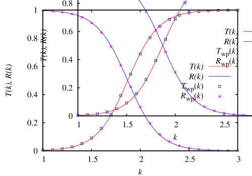
Figure 3: The transmission and reflection coefficients as a function of $k$ when $\beta=1$, $\lambda=2.5$, $m=1$, and $\sigma_{0}=10$. The subscript “wp” indicates that the coefficients are obtained from the emerging wavepackets. The quantities without subscripts are calculated using the time-independent method.

V.3 Long-time behavior of decay of quasi-stable system

There are few analytically solvable models of the time evolution of unstable quantum systems van Dijk and Nogami (2002, 2003b). Realistic systems need to be solved numerically. Long-time calculations are required for systems which require both nuclear and atomic time-scales such as ionization and bremsstrahlung due to radioactive decay of the nucleus of an atom Kataoka et al. (2000); Bertulani et al. (1999); Ş. Mişicu et al. (2001). To study the short-time anomalous power law behavior of the decay and the long-time inverse-power law behavior the method of this paper is appropriate. This is especially relevant because of the recently observed violation of the exponential-decay law at long times Rothe et al. (2006).

To illustrate the numerical method discussed in this paper as applied to decaying systems let us consider a variant of the model with a $\delta$-shell potential Winter (1961), but with the $\delta$ function replaced by a gaussian. Thus in the $S$ partial wave of a spherical system the potential is

$$V(\rho)=\frac{\lambda}{w\sqrt{\pi}}\exp{[-(\rho-a)^{2}/w^{2}]},$$ (5.8)

where $\rho$ is the radial coordinate. This potential reduces to the $\delta$-shell potential, $V_{\delta}(\rho)=\lambda\delta(\rho-a)$ when $w\rightarrow 0$. For small but finite values of $w$ this potential leads to scattering results which are good approximations of those of the $\delta$-shell interaction . Initially the quantum system is in the state

$$\psi(\rho,0)=\sqrt{2/a}\sin{(\pi\rho/a)}.$$ (5.9)

In our example we take $\hbar=1$, $\lambda=3$, $m={1\over 2}$, $a=1$ and $w=0.10$. Using the numerical method of this paper, including the modification of matrix $A$ as described in Sec. IV.2 to take care of the boundary conditions at $\rho=0$, we determine the wave function at later times, i.e., $\psi(\rho,t)$. From that we obtain the nonescape probability, as a function of $t$, $P(t)=\int_{0}^{a}|\psi(\rho,t)|^{2}\ d\rho$, which is shown in Fig. 4.

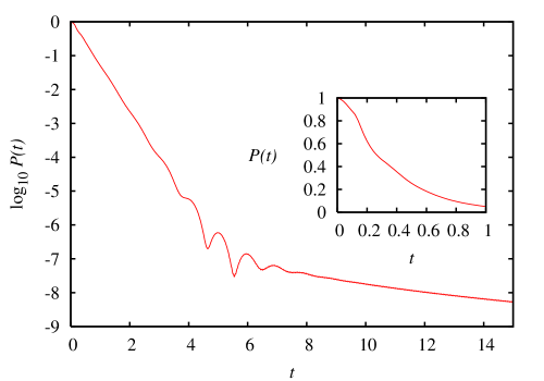
Figure 4: The nonescape probability as a function of time for the interaction with $\lambda=3$, $a=1$, and $w=0.10$. We also take $\hbar=1$ and $m={1\over 2}$.

It clearly shows the exponential decay-region in time, the inverse power-law behavior for long times, the deviation from exponential decay at short times, and the transition regions Winter (1961).

The quadratic short-time behavior is seen in Fig. 4 as is the inverse power law behavior at long times Khaflin (1958). Remarkably the decaying system can be studied in this manner for a time exceeding thirty half-lives. In Fig. 5 we plot the square of the absolute value of the wave function at times $t=5,10,15$.

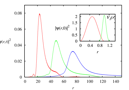
Figure 5: The square of the absolute value of the wave function as a function of $\rho$ at times $t=5,10,15$ for the same parameters apply as in Fig. 4. The insert gives the $t=0$ graph as well as the scaled potential, $V_{1}(\rho)=V(\rho)/8$.

Notice that the wave function (packet) has three distinct regions: a precursor due to energy components of the initial wave function larger than that associated with the exponential decay, the main packet which corresponds to the exponential decay at the resonance energy, and the follower, which is a small blip that stretches in time (travels more slowly) and is due to energy components in the initial wave function which have lower energy that the resonance energy. If the maximum spatial coordinate, which is set at 800 for this calculation, were set at a smaller value, say 400, then one observes a fuzziness in the precursor of the right-most wave function. This can be attributed to the finite space in which the wavepacket travels so that the fast precursor has been partially reflected from the right boundary and interferes with the wave front of the main wavepacket. The numerical parameters for this calculation are $\Delta\rho=0.1$, $\Delta t=0.02$, $r=20$ and $M=20$.

VI Remarks

The generalized CN method that we have presented in this paper gives many orders of magnitude improvement in the precision of the results and several orders of magnitude in the computational time required to obtain the results. Clearly, since this method enhances the efficiency of the numerical calculations, it can be a significant tool for studying time-dependent processes. It goes beyond the improvement of Ref. Ş. Mişicu et al. (2001) in a systematic way. It also is an advance over the method of Ref. Moyer (2004), since the Numerov method has an error ${\cal O}((\Delta x)^{6})$, and it is difficult to see how it can be generalized systematically to higher order spatial errors. The generalized time evolution algorithm can be applied to Moyer’s Moyer (2004) method.

We have applied the method for $r$ and $M$ up to and including 20 for both. Having achieved significant improvements with these values of $r$ and $M$ we did not consider larger values although there does not seem to be a practical reason that this cannot be done. Although the approach seems to saturate at $r$ around 10 (see Table 3), there is no visible saturation in the time-evolution part of the problem. One would expect higher orders of spatial errors to be significant when the wave function and/or the potential has large spatial fluctuations. Even so, at $r=7$ we are using a 15-point formula for the second-order spatial derivative, and it is surprising that a smaller number of points in the formula is not sufficient for optimal results in this case. It should be noted that the higher order method as discussed in this paper are suitable only for well-behaved, sufficiently differentiable solutions; these occur when the potential function is well behaved. As the authors of Ref. Press et al. (1992) point out for singular functions higher-order methods do not necessarily lead to greater accuracy.

It should be noted that in this paper we consider primarily one-dimensional systems, but the method applies equally well to partial-wave equations of two- or three-dimensional systems. The study of the decaying quasi-stable state is an example of the latter.

An interesting avenue to investigate further is the impact that this approach may have on two- or three-dimensional systems, where the number of variables involved is equal to the dimension. The Peaceman-Rachford-type approach Peaceman and H. H. Rachford (1955), also known as the alternating-direction implicit method, of factoring the approximation of the time evolution operator may apply as it did in Refs. Galbraith et al. (1984); Kulander et al. (1982) or more recently in, for example, Refs. Shon et al. (2000); Ishikawa (2004). Using the Crank-Nicolson method the authors of Refs. Galbraith et al. (1984); Kulander et al. (1982) show that in two dimension the kinetic energy parts of the evolution operator factorizes. Whether such factorization can be generalized in the spirit of the method of this paper is under investigation.

Calculations on one-dimensional multichannel systems indicate that this approach also leads to substantially greater efficiencies.

Preliminary studies with the Numerov spatial integration scheme Moyer (2004) and the generalized time evolution as described in this work indicate that significant improvements occur if one incorporates appropriate changes in the spatial step size for different regions of space. This is important in the case of discontinuous potentials and potentials that have great variation in some region and little or no variation in other regions. Furthermore it is well known that the wavepacket has large fluctuation in a (short-range) potential region and little variation in the asymptotic regions. A great savings in computational time can be achieved by using different space-step sizes in the different regions. One needs to investigate whether such variable step size can be incorporated in the generalized spatial integration scheme of this paper. The approach that dealt with the discontinuous first- or second-order derivative in this paper and Ref. Muller (1999) is worth exploring. We intend to study this in the future.