Classes of complex networks defined
by role-to-role connectivity profiles
Interactions between units in phyical, biological, technological, and social systems usually give rise to intrincate networks with non-trivial structure, which critically affects the dynamics and properties of the system. The focus of most current research on complex networks is on global network properties. A caveat of this approach is that the relevance of global properties hinges on the premise that networks are homogeneous, whereas most real-world networks have a markedly modular structure. Here, we report that networks with different functions, including the Internet, metabolic, air transportation, and protein interaction networks, have distinct patterns of connections among nodes with different roles, and that, as a consequence, complex networks can be classified into two distinct functional classes based on their link type frequency. Importantly, we demonstrate that the above structural features cannot be captured by means of often studied global properties.
The structure of complex networks 1, 2 is typically characterized in terms of global properties, such as the average shortest path length between nodes 3, the clustering coefficient 3, the assortativity 4 and other measures of degree-degree correlations 5, 6, and, especially, the degree distribution 7, 8. However, these global quantities are truly informative only when one of two strict conditions is fulfilled: (i) the network lacks a modular structure 9, 10, 11, 12, 13, 14, or (ii) the network has a modular structure but (ii.a) all modules were formed according to the same mechanisms, and therefore have similar properties, and (ii.b) the interface between modules is statistically similar to the bulk of the modules, except for the density of links. If neither of these two conditions is fulfilled, then any theory proposed to explain, for example, a scale-free degree distribution needs to take into account the modular structure of the network.
To our knowledge, no real-world network has been shown to fulfill either of the two conditions above; this implies that global properties may sometimes fail to provide insight into the mechanisms responsible for the formation or growth of these networks. Alternative approaches that take into consideration the modular structure of real-world complex networks are therefore necessary. One such approach is to group nodes into a small number of roles, according to their pattern of intra- and inter-module connections 11, 12, 13. Recently, we demonstrated that the role of a node conveys significant information about the importance of the node, and about the evolutionary pressures acting on it 11, 13. Here, we demonstrate that modular networks can be classified into distinct functional classes according to the patterns of role-to-role connections, and that the definition of link types can help us understand the function and properties of a particular class of networks.
Modularity of complex networks
We analyze four different types of real-world networks—metabolic networks 11, 15, 16, protein interactomes 17, 18, 19, 20, global and regional air transportation networks 13, 21, 22, and the Internet at the autonomous system (AS) level 5, 23 (Table 1 and Supplementary discussion). To determine and quantify the modular structure of these networks, we use simulated annealing 24 to find the optimal partition of the network into modules 11, 12, 25 (Methods). We then assess the significance of the modular structure of each network by comparing it to a randomization of the same network 25. We find that all networks studied have a significant modular structure (Table 1). Modules correspond to functional units in biological networks 11, 20 and to geo-political units in air transportation networks 13 and, probably, in the Internet 26.
To assess whether global average properties are appropriate to describe the structure of these networks, we compare global average properties of the networks to the corresponding module-specific averages; specifically, we focus on the degree, the clustering coefficient, and the normalized clustering coefficient. We find that the average degree of the network is not representative of individual-module average degrees for air transportation networks (Table 2). Most importantly, the global clustering coefficient is not representative of individual-module clustering coefficients for any network (except, maybe, for one out of 18 metabolic networks).
Role-based description of complex networks
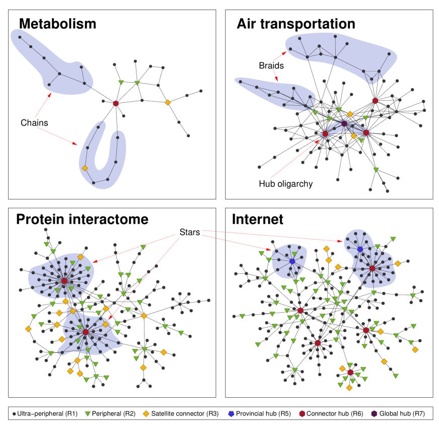
As an alternative to the average description approach, we determine the role of each node according to two properties 11, 12 (Methods): the relative within-module degree , which quantifies how well connected a node is to other nodes in their module, and the participation coefficient , which quantifies to what extent the node connects to different modules. We classify as non-hubs those nodes that have low within-module degree (). Depending on the fraction of connections they have to other modules, non-hubs are further subdivided into 11, 12: (R1) ultra-peripheral nodes, that is, nodes with all their links within their own module; (R2) peripheral nodes, that is, nodes with most links within their module; (R3) satellite connectors, that is, nodes with a high fraction of their links to other modules; and (R4) kinless nodes, that is, nodes with links homogeneously distributed among all modules. We classify as hubs those nodes that have high within-module degree (). Similar to non-hubs, hubs are divided according to their participation coefficient into: (R5) provincial hubs, that is, hubs with the vast majority of links within their module; (R6) connector hubs, that is, hubs with many links to most of the other modules; and (R7) global hubs, that is, hubs with links homogeneously distributed among all modules.
Although the full rationale for this particular definition of the roles has been given elsewhere 12, it is important to highlight a few properties of our classification scheme. Nodes in real and model networks, especially non-hubs, do not fill uniformly the -plane; our role classification scheme arises from the fact that nodes tend to congregate into a small number of densely populated regions of this space, with boundaries between these regions having low density of nodes. Additionally, especially for hubs, boundaries coincide with well defined connectivity patterns; for example, nodes at the boundary between connector hubs (R6) and global hubs (R7) would have approximately half of their links in one module, and the other half perfectly spread in other modules. Importantly, other definitions of the roles do not alter the results we report below (see Supplementary Information).
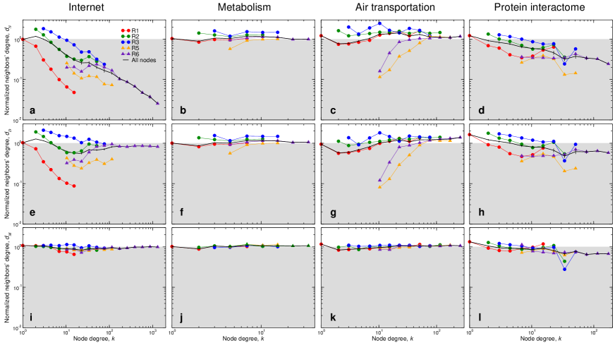
We investigate how our definition of roles relates to global network properties, and to what extent global network properties are representative of nodes with different roles. Since some simple properties like the degree and the clustering coefficient trivially depend on a node’s role, we focus on degree-degree correlations 4, 5, 19, 27, 28, 6. Specifically, we address two questions: (i) whether nodes with the same degree but different roles have the same or different correlations; and (ii) to what extent the observed degree-degree correlations are a byproduct of the modular structure of the network.
To answer these questions, we start by considering the Internet at the AS level (Fig. 1). Nodes with degree can be either ultra-peripheral (R1, if they have all connections in the same module), peripheral (R2, if they have two connections in one module and one in another), or satellite connectors (R3, if the three connections are to different modules). A separate analysis for each role reveals that the average degree of the neighbors of a node 5 with degree strongly depends on the role of the node. For an instance of the 1998 Internet, for example, for ultra-peripheral nodes, for peripheral nodes, and for satellite connectors. We observe a dependence of on the nodes’ role for all the networks studied here (Fig. 1a-d).
Regarding the second question, initial research showed 5 that for the Internet at the AS level . It was later pointed out 28, 27 that any network with the same degree distribution as the Internet should display a similar scaling. In other words, the degree distribution of the network is responsible for most of the observed correlations. However, the degree distribution alone does not account for all the observed correlations 28 (Fig. 1e). In contrast, the modular structure of the network does account for most of the remaining degree-degree correlations observed in the topology of the Internet (Fig. 1i). Similarly, the modular structure accounts for the degree-degree correlations in metabolic networks and the air transportation network, and for most of the correlations in protein interaction networks (Fig. 1i-l).
Role-to-role connectivity profiles
The findings we reported so far suggest that, once the degree distribution and the modular structure are fixed, real networks have no additional internal structure. This, however, contradicts our intuition that networks with different growth mechanisms and functional needs should have distinct connection patterns between nodes playing different roles. To investigate this possibility, we systematically analyze how nodes connect to one another depending on their roles.
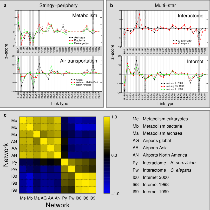
For each network, we calculate the number of links between nodes belonging to roles and , and compare this number to the number of such links in a properly randomized network (Methods). As in previous work 19, 29, 28, 30, we use the -score to obtain a profile of over- and under-representation of link types (Fig. 2), which enables us to compare different networks. We quantify the overall similarity between two profiles and by the scalar product between these profiles (Methods). In Fig. 2, we show that networks of the same type have highly correlated profiles, while networks of different types have weaker correlations and, at times, even strong anti-correlations (Fig. 2c).
The networks considered fall into two main classes, one comprising metabolic and air transportation networks, and another comprising protein interactomes and the Internet. The main difference between the two groups is the pattern of links between: (i) ultra-peripheral nodes (links of type R1-R1), and (ii) connector hubs and other hubs (links of types R5-R6 and R6-R6). These link types are over-represented for networks in the first class (except links of type R6-R6 in metabolic networks), and under-represented for networks in the second class.
We denote the first class as the stringy-periphery class (Fig. 3a, b). In networks of this class, ultra-peripheral nodes are more connected to one another than one would expect from chance, which results in long “chains” of ultra-peripheral nodes. In metabolic networks, these chains correspond to loop-less pathways that, for example, degrade a complex metabolite into simpler molecules. In the air transportation network, due to the higher overall connectivity of the network, chains contain short loops and resemble “braids.” Stringy-periphery networks also have a core of hubs, which we call the hub oligarchy, that are directly reachable from one another (links of type R5-R6 in metabolic and air transportation networks, and R6-R6 in air transportation networks). Moreover, connector hubs are less connected to ultra-peripheral nodes (R1) than expected by chance alone.
We denote the second class as the multi-star class (Fig. 3c, d). The multi-star class comprises the protein interactomes and the Internet, and has the opposite signature to the stringy-periphery class. Links of type R1-R1 (between ultra-peripheral nodes) are under-represented, whereas links of type R1-R5 (between ultra-peripheral nodes and provincial hubs) are, over-represented, giving rise to modules with indirectly-connected “star-like” structures. Similarly, connector hubs are less connected to one another than one would expect, which means that these networks depend on satellite connectors to bridge connector hubs and modules.
Our findings confirm and clarify previous results in the literature. For example, the under-representation of R6-R6 links in protein interactomes is consistent with previous results suggesting a tendency for hubs to “repel” each other in these networks 19, 6. Similarly, the role-to-role connectivity profile of the Internet is consistent with the existence of a hierarchy of types of nodes 28. This hierarchy comprises end users, regional providers, and global providers, which we hypothesize correspond correspond to roles R1-R2, R5, and R6 respectively. The role-to-role connectivity profiles are consistent with a scenario in which end users connect mostly to regional providers, and in which global providers connect with each other indirectly through satellite connectors (R3), with few connections but probably large bandwidth.
By considering the modular structure of the networks and the extra dimension introduced by the participation coefficient, however, our approach provides novel insights into the relationship between structure and function in complex networks. For example, by considering the absolute degree alone nodes with roles R5 and R6 in protein interactomes are indistinguishable from each other: in S. cerevisiae, and , whereas the average degree for the whole network is . Still, links R5-R5 between provincial hubs, unlike R6-R6 links, are not under-represented. In general, the different connection patterns of R5 and R6 (or R1 and R2) proteins enables us to hypothesize that they play distinct biological roles, with R6 proteins likely being much more important 31.
A closer look at the air transportation network also helps to show that important structural properties may be left unexplained by focusing on degree alone, as well as to stress the importance of the relative within-module degree as opposed to the degree. Johannesburg, in South Africa, has degree 84, which is 23% smaller than the degree of Cincinnati in the U.S., 109. Still, one can fly from most capitals in the world to Johannesburg but not to Cincinnati. There are two main reasons for this. First, while Johannesburg is the most connected city in its region (sub-Saharan Africa), Cincinnati (North America) is not; this effect is captured by the within-module relative degree, which is 9.3 for Johannesburg and 4.3 for Cincinnati. Second, Johannesburg has many connections to other regions, whereas Cincinnati does not; this effect is captured by the participation coefficient, which is 0.52 for Johannesburg and 0.05 for Cincinnati. As a result, Johannesburg is a global hub (R6) in our classification, whereas Cincinnati is a provincial hub (R5). One can thus understand why R6-R6 connections are over-represented in air transportation networks (most global hubs are connected to one another), whereas R5-R5 are not (most provincial hubs are poorly connected to provincial hubs in other regions). In general, our approach shows why the behavior of R5 and R6 nodes is so different in air transportation networks, which cannot be understood from the degree of the nodes alone.
Conclusion
We have shown that global properties that do not take into account the modular organization of the network may sometimes fail to capture potentially important structural features; although all networks (except, maybe, the protein interactomes) show no degree-degree correlations when compared to the appropriate ensemble of random networks, they all have clearly distinctive properties in terms of how nodes with certain roles are connected to each other. Our results thus call attention to the need to develop new approaches that will enable us to better understand the structure and evolution of real-world complex networks.
Additionally, our findings demonstrate that networks with the same functional needs and growth mechanisms have similar patterns of connections between nodes with different roles. Attempts to divide complex networks into “classes” or “families” have been made before, for example in terms of the degree distribution 8 and in terms of the relative abundance of certain subgraphs or motifs 29, 30. Our work here complements those attempts, and is the first one to build on the crucial fact that most real-world networks display a markedly modular structure.
Although we cannot put forward a theory for the division of the networks into two classes, we hypothesize that it might be related to the fact that networks in the stringy-periphery class are transportation networks, in which strict conservation laws must be fulfilled. Indeed, for transportation systems it has been shown that, under quite general conditions, a hub oligarchy is the the most efficient organization 32. Conversely, both protein interactomes and the Internet can be seen as signaling networks, which do not obey conservation laws.
Methods
Module identification
The modularity of a partition of a network into modules is 10
| (1) |
where is the number of non-empty modules (smaller than or equal to the number of nodes in the network), is the number of links in the network, is the number of links between nodes in module , and is the sum of the degrees of the nodes in module . The objective of a module identification algorithm is to find the partition that yields the largest modularity . Note that is only constrained to be , but is otherwise selected by the optimization algorithm so that is maximum. The problem of identifying the optimal partition is analogous to finding the ground state of a disordered system with Hamiltonian . 25
Role definition
We determine the role of each node according to two properties 11, 12: the relative within-module degree and the participation coefficient . The within-module degree -score measures how “well-connected” node is to other nodes in the module compared to those other nodes, and is defined as
| (2) |
where is the number of links of node to nodes in module , is the module to which node belongs, and the averages are taken over all nodes in module .
The participation coefficient quantifies to what extent a node connects to different modules We define the participation coefficient of node as
| (3) |
where is the number of links of node to nodes in module , and is the total degree of node . The participation coefficient of a node is therefore close to one if its links are uniformly distributed among all the modules and zero if all its links are within its own module.
We classify as non-hubs those nodes that have low within-module degree (). Depending on the amount of connections they have to other modules, non-hubs are further subdivided into 11, 12: (R1) ultra-peripheral nodes, that is, nodes with all their links within their own module (); (R2) peripheral nodes, that is, nodes with most links within their module (); (R3) satellite connectors, that is, nodes with a high fraction of their links to other modules (); and (R4) kinless nodes, that is, nodes with links homogeneously distributed among all modules (). We classify as hubs those nodes that have high within-module degree (). Similar to non-hubs, hubs are divided according to their participation coefficient into: (R5) provincial hubs, that is, hubs with the vast majority of links within their module (); (R6) connector hubs, that is, hubs with many links to most of the other modules (); and (R7) global hubs, that is, hubs with links homogeneously distributed among all modules ().
Network randomization and statistical ensembles
We use two different ensembles of random networks 19, 28. In the first ensemble, which we denote by , we only preserve the degree sequence of the original network; in the second ensemble, denoted , we preserve both the degree sequence and the modular structure of the network. Averages over the first and second ensembles are denoted and , respectively.
To generate random networks in ensemble , we randomize all the links in the network while preserving the degree of each node. To uniformly sample all possible networks, we use the Markov-chain Monte Carlo switching algorithm 19, 33. In this algorithm, one repeatedly selects random pairs of links, for example and , and swaps one of the ends of each link, so that the links become and .
To generate random networks in ensemble , we restrict the Markov-chain Monte Carlo switching algorithm 28 to pairs of links that connect nodes in the same pair of modules, that is, we apply the Markov-chain Monte Carlo switching algorithm independently to links whose ends are in modules 1 and 1, 1 and 2, and so forth for all pairs of modules. This method guarantees that, with the same partition as the original network, the modularity of the randomized network is the same as that of the original network (since the number of links between each pair of modules is unchanged) and that the role of each node is also preserved.
To investigate whether global properties are representative of module-specific properties, we focus on degree , clustering coefficient , and normalized clustering coefficient . For each module in the network, comprising nodes, we compute the average of each property in the module (for example, ). Additionally, we compute the distribution of such averages for random modules, which we obtain by randomly selecting groups of nodes. If the empirical module average falls outside of the 95% probability of the distribution for the random modules, we consider that the global average is not representative of the module average. We finally compute the fraction of modules that are not properly described by the global average.
To study degree-degree correlations, we consider the average degree of the nearest neighbors of each node . We define the normalized nearest neighbors’ degree as the ratio of and: (i) the average value of in the network
| (4) |
where is the number of nodes in the network; (ii) the expected value of in the ensemble of networks with fixed degree sequence
| (5) |
and (iii) the expected value of in the ensemble of networks with fixed degree sequence and modular structure
| (6) |
Note that, in spite of the similar notation, the meaning of is somewhat different from the other two because the normalization involves an average over nodes, while in and the normalization involves averages over an ensemble of randomized networks.
To obtain the role-to-role connectivity profiles, we calculate the -score 19, 29, 28, 30 of the number of links between nodes with roles and as
| (7) |
where is the number of links between nodes with roles and . To obtain better statistics and an estimation of the error in the -score, we carry out this process for several partitions of each network.
To evaluate the similarity between two -score profiles and , we use the scalar product
| (8) |
where is the standard deviation of the elements in .
References
- Newman 2003 Newman, M. E. J. The structure and function of complex networks. SIAM Review 45, 167–256 (2003).
- Amaral & Ottino 2004 Amaral, L. A. N. & Ottino, J. Complex networks: Augmenting the framework for the study of complex systems. Eur. Phys. J. B 38, 147–162 (2004).
- Watts & Strogatz 1998 Watts, D. J. & Strogatz, S. H. Collective dynamics of ‘small-world’ networks. Nature 393, 440–442 (1998).
- Newman 2002 Newman, M. E. J. Assortative mixing in networks. Phys. Rev. Lett. 89, art. no. 208701 (2002).
- Pastor-Satorras et al. 2001 Pastor-Satorras, R., Vázquez, A. & Vespignani, A. Dynamical and correlation properties of the Internet. Phys. Rev. Lett. 87, art. no. 258701 (2001).
- Colizza et al. 2006 Colizza, V., Flammini, A., Serrano, M. A. & Vespignani, A. Detecting rich-club ordering in complex networks. Nature Phys. 2, 110–115 (2006).
- Barabási & Albert 1999 Barabási, A.-L. & Albert, R. Emergenge of scaling in random networks. Science 286, 509–512 (1999).
- Amaral et al. 2000 Amaral, L. A. N., Scala, A., Barthélémy, M. & Stanley, H. E. Classes of small-world networks. Proc. Natl. Acad. Sci. USA 97, 11149–11152 (2000).
- Girvan & Newman 2002 Girvan, M. & Newman, M. E. J. Community structure in social and biological networks. Proc. Natl. Acad. Sci. USA 99, 7821–7826 (2002).
- Newman & Girvan 2004 Newman, M. E. J. & Girvan, M. Finding and evaluating community structure in networks. Phys. Rev. E 69, art. no. 026113 (2004).
- Guimerà & Amaral 2005a Guimerà, R. & Amaral, L. A. N. Functional cartography of complex metabolic networks. Nature 433, 895–900 (2005a).
- Guimerà & Amaral 2005b Guimerà, R. & Amaral, L. A. N. Cartography of complex networks: modules and universal roles. J. Stat. Mech.: Theor. Exp. P02001 (2005b).
- Guimerà et al. 2005 Guimerà, R., Mossa, S., Turtschi, A. & Amaral, L. A. N. The worldwide air transportation network: Anomalous centrality, community structure, and cities’ global roles. Proc. Natl. Acad. Sci. USA 102, 7794–7799 (2005).
- Danon et al. 2005 Danon, L., Díaz-Guilera, A., Duch, J. & Arenas, A. Comparing community structure identification. J. Stat. Mech.: Theor. Exp. P09008 (2005).
- Jeong et al. 2000 Jeong, H., Tombor, B., Albert, R., Oltvai, Z. N. & Barabási, A.-L. The large-scale organization of metabolic networks. Nature 407, 651–654 (2000).
- Wagner & Fell 2001 Wagner, A. & Fell, D. A. The small world inside large metabolic networks. Proc. Roy. Soc. B 268, 1803–1810 (2001).
- Uetz et al. 2000 Uetz, P. et al. A comprehensive analysis of protein-protein interactions in Saccharomyces cerevisiae. Nature 403, 623–627 (2000).
- Jeong et al. 2001 Jeong, H., Mason, S. P., Barabási, A.-L. & Oltvai, Z. N. Lethality and centrality in protein networks. Nature 411, 41–42 (2001).
- Maslov & Sneppen 2002 Maslov, S. & Sneppen, K. Specificity and stability in topology of protein networks. Science 296, 910–913 (2002).
- Li et al. 2004 Li, S. et al. A map of the interactome network of the metazoan C. elegans. Science 303, 540–543 (2004).
- Barrat et al. 2004 Barrat, A., Barthélemy, M., Pastor-Satorras, R. & Vespignani, A. The architecture of complex weighted networks. Proc. Natl. Acad. Sci. USA 101, 3747–3752 (2004).
- Li & Cai 2004 Li, W. & Cai, X. Statistical analysis of airport network of China. Phys. Rev. E 69, art. no. 046106 (2004).
- Vázquez et al. 2002 Vázquez, A., Pastor-Satorras, R. & Vespignani, A. Large-scale topological and dynamical properties of the Internet. Phys. Rev. E 65, art. no. 066130 (2002).
- Kirkpatrick et al. 1983 Kirkpatrick, S., Gelatt, C. D. & Vecchi, M. P. Optimization by simulated annealing. Science 220, 671–680 (1983).
- Guimerà et al. 2004 Guimerà, R., Sales-Pardo, M. & Amaral, L. A. N. Modularity from fluctuations in random graphs and complex networks. Phys. Rev. E 70, art. no. 025101 (2004).
- Eriksen et al. 2003 Eriksen, K. A., Simonsen, I., Maslov, S. & Sneppen, K. Modularity and extreme edges of the Internet. Phys. Rev. Lett. 90, art. no. 148701 (2003).
- Park & Newman 2003 Park, J. & Newman, M. E. J. Origin of degree correlations in the Internet and other networks. Phys. Rev. E 68, art. no. 026112 (2003).
- Maslov et al. 2004 Maslov, S., Sneppen, K. & Zaliznyak, A. Detection of topological patterns in complex networks: correlation profile of the internet. Physica A 333, 529–540 (2004).
- Milo et al. 2002 Milo, R. et al. Network motifs: simple building blocks of complex networks. Science 298, 824–827 (2002).
- Milo et al. 2004 Milo, R. et al. Superfamilies of evolved and designed networks. Science 303, 1538–1542 (2004).
- Han et al. 2004 Han, J.-D. J. et al. Evidence for dynamically organized modularity in the yeast protein-protein interaction network. Nature 430, 88–93 (2004).
- Arenas et al. 2003 Arenas, A., Cabrales, A., Díaz-Guilera, A., Guimerà, R. & Vega-Redondo, F. Search and congestion in complex networks. In Statistical Mechanics of Complex Networks (eds. Pastor-Satorras, R., Rubi, M. & Díaz-Guilera, A.), Lecture Notes in Physics (Springer Verlag, Berlin, 2003).
- Itzkovitz et al. 2004 Itzkovitz, S., Milo, R., Kashtan, N., Newman, M. E. J. & Alon, U. Reply to “Comment on ‘Subgraphs in random networks’ ”. Phys. Rev. E 70, art. no. 058102 (2004).
Correspondence and requests for materials should be addressed to R. G.
Acknowledgments We thank R.D. Malmgren, E.N. Sawardecker, S.M.D. Seaver, D.B. Stouffer, and M.J. Stringer for useful comments and suggestions. R.G. and M.S.-P. thank the Fulbright Program. L.A.N.A. gratefully acknowledges the support of a NIH/NIGMS K-25 award, of NSF award SBE 0624318, of the J.S. McDonnell Foundation, and of the W. M. Keck Foundation.
| Network type | Network | Nodes | Links | |||
| Metabolism Archaea | A. fulgidus | 303 | 366 | 16 | 0.813 | 0.746 (0.005) |
| A. pernix | 300 | 387 | 14 | 0.797 | 0.711 (0.006) | |
| M. jannaschii | 223 | 277 | 14 | 0.813 | 0.720 (0.003) | |
| P. aerophilum | 335 | 421 | 15 | 0.811 | 0.731 (0.004) | |
| P. furiosus | 302 | 384 | 16 | 0.813 | 0.720 (0.007) | |
| S. solfataricus | 367 | 455 | 17 | 0.813 | 0.736 (0.006) | |
| Metabolism Bacteria | B. subtilis | 649 | 863 | 20 | 0.815 | 0.724 (0.003) |
| E. coli | 739 | 1009 | 17 | 0.810 | 0.711 (0.003) | |
| F. nucleatum | 378 | 473 | 16 | 0.816 | 0.734 (0.004) | |
| H. pylory | 360 | 438 | 15 | 0.837 | 0.746 (0.006) | |
| M. leprae | 451 | 578 | 16 | 0.814 | 0.732 (0.005) | |
| T. elongatus | 448 | 546 | 17 | 0.830 | 0.755 (0.006) | |
| Metabolism Eukaryotes | A. thaliana | 607 | 792 | 18 | 0.825 | 0.728 (0.003) |
| C. elegans | 431 | 569 | 17 | 0.818 | 0.714 (0.004) | |
| H. sapiens | 792 | 1056 | 23 | 0.842 | 0.727 (0.003) | |
| P. falciparum | 280 | 363 | 12 | 0.815 | 0.708 (0.006) | |
| S. cerevisiae | 570 | 776 | 17 | 0.814 | 0.708 (0.003) | |
| S. pombe | 503 | 664 | 18 | 0.827 | 0.721 (0.003) | |
| Air transportation | Global | 3618 | 14142 | 25 | 0.706 | 0.3111 (0.0009) |
| Asia & Middle East | 706 | 2572 | 10 | 0.642 | 0.325 (0.002) | |
| North America | 940 | 3446 | 12 | 0.522 | 0.3111 (0.0005) | |
| Interactome | S. cerevisiae | 1458 | 1948 | 25 | 0.820 | 0.707 (0.002) |
| C. elegans | 2889 | 5188 | 28 | 0.688 | 0.561 (0.002) | |
| Internet | 1998 | 3216 | 5705 | 17 | 0.625 | 0.5365 (0.0011) |
| 1999 | 4513 | 8374 | 18 | 0.620 | 0.5227 (0.0007) | |
| 2000 | 6474 | 12572 | 22 | 0.631 | 0.5042 (0.0008) |
| Network type | Network | |||
|---|---|---|---|---|
| Metabolism Archaea | A. fulgidus | 0.02 (0.03) | 0.125 (0.0) | 0.10 (0.03) |
| A. pernix | 0.0 (0.0) | 0.17 (0.04) | 0.18 (0.04) | |
| M. jannaschii | 0.0 (0.0) | 0.27 (0.03) | 0.27 (0.02) | |
| P. aerophilum | 0.03 (0.03) | 0.22 (0.06) | 0.16 (0.05) | |
| P. furiosus | 0.02 (0.03) | 0.27 (0.04) | 0.24 (0.06) | |
| S. solfataricus | 0.02 (0.03) | 0.15 (0.04) | 0.11 (0.04) | |
| Metabolism Bacteria | B. subtilis | 0.02 (0.02) | 0.22 (0.06) | 0.19 (0.04) |
| E. coli | 0.02 (0.04) | 0.27 (0.06) | 0.29 (0.04) | |
| F. nucleatum | 0.0 (0.0) | 0.06 (0.02) | 0.06 (0.03) | |
| H. pylori | 0.08 (0.05) | 0.28 (0.04) | 0.26 (0.03) | |
| M. leprae | 0.0 (0.0) | 0.28 (0.05) | 0.27 (0.04) | |
| T. elongatus | 0.01 (0.02) | 0.11 (0.03) | 0.12 (0.04) | |
| Metabolism Eukaryotes | A. thaliana | 0.04 (0.03) | 0.29 (0.06) | 0.29 (0.07) |
| C. elegans | 0.064 (0.004) | 0.31 (0.03) | 0.30 (0.03) | |
| H. sapiens | 0.08 (0.03) | 0.45 (0.04) | 0.41 (0.05) | |
| P. falciparum | 0.084 (0.002) | 0.23 (0.03) | 0.24 (0.02) | |
| S. cerevisiae | 0.09 (0.04) | 0.24 (0.05) | 0.23 (0.05) | |
| S. pombe | 0.059 (0.003) | 0.37 (0.06) | 0.36 (0.06) | |
| Air transportation | Global | 0.41 (0.05) | 0.531 (0.010) | 0.43 (0.02) |
| Asia & Middle East | 0.40 (0.10) | 0.26 (0.04) | 0.21 (0.05) | |
| North America | 0.37 (0.03) | 0.40 (0.04) | 0.47 (0.05) | |
| Interactome | S. cerevisiae | 0.0 (0.0) | 0.25 (0.09) | 0.67 (0.04) |
| C. elegans | 0.042 (0.014) | 0.47 (0.06) | 0.33 (0.04) | |
| Internet | 1998 | 0.064 (0.005) | 0.77 (0.05) | 0.77 (0.06) |
| 1999 | 0.0 (0.0) | 0.85 (0.03) | 0.83 (0.05) | |
| 2000 | 0.0 (0.0) | 0.77 (0.04) | 0.76 (0.07) |