Fractal templates in the escape dynamics of trapped ultracold atoms

Abstract

We consider the dynamic escape of a small packet of ultracold atoms launched from within an optical dipole trap. Based on a theoretical analysis of the underlying nonlinear dynamics, we predict that fractal behavior can be seen in the escape data. This data would be collected by measuring the time-dependent escape rate for packets launched over a range of angles. This fractal pattern is particularly well resolved below the Bose-Einstein transition temperature—a direct result of the extreme phase space localization of the condensate. We predict that several self-similar layers of this novel fractal should be measurable and we explain how this fractal pattern can be predicted and analyzed with recently developed techniques in symbolic dynamics.

Chaotic escape is a widespread transport process underlying such diverse phenomena as conductance through ballistic microstructures Taylor03 , emission from deformed micro-disk semiconductor lasers Gmachl98 , molecular scattering and dissociation Molecules , celestial transport Celestial , and atomic ionization ChaoticIonization ; Mitchell04 . We have been particularly motivated by the chaotic ionization of hydrogen in applied parallel electric and magnetic fields, for which a recent theoretical analysis Mitchell04 predicts that the time-spectrum for ionization will display a chaos-induced train of electron pulses. This prediction is based on classical ionizing trajectories (Fig. 1a), which propagate from the nucleus into the ionization channel, via the Stark saddle. These trajectories exhibit fractal self-similarity, which is reflected in the pulse train. This prediction has been recently confirmed by full quantum computations Turker . However, the experimental observation of these chaos-induced pulse trains remains unrealized.

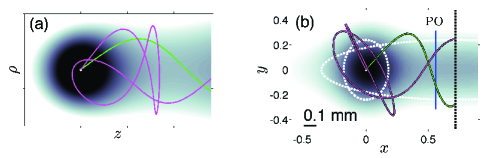
Figure 1: a) The potential energy for a hydrogenic electron in applied parallel electric and magnetic fields. Two ionizing trajectories are shown. b) The double-Gaussian potential. Gaussian widths are indicated by the dashed ellipses.

In this Letter, we propose an alternate physical system—the escape of ultracold atoms in specially tailored optical dipole traps—that exhibits similar escape dynamics. However, we show that the flexibility and control afforded by cold atoms, especially in engineering the initial state, should permit the direct imaging of fractals in the escape dynamics, including novel self-similar features. Furthermore, we show how this self-similarity can be analyzed using a recently developed symbolic formalism. Fundamentally, these fractals result from homoclinic tangles Wiggins92 —a general mechanism for phase space transport. Hence this Letter suggests that cold atoms could serve as a unique high-precision experimental probe of this mechanism. Finally, the cold atom experiments discussed here are readily feasible with present-day experimental configurations and should prove easier to realize than the previously mentioned ionization experiments.

Recent experiments from the Raizen Raizen01 and Davidson Davidson01 groups have made first steps along these lines. They independently measured the long-time survival probability for ultracold atoms escaping through a hole in an optical billiard, demonstrating the distinction between regular and chaotic escape dynamics. In contrast, our Letter focuses on the short- to intermediate-time dynamics, where fundamentally distinct phenomena, such as fractal self-similarity, are predicted to appear.

The double-Gaussian trap: We consider a dipole potential consisting of two overlapping Gaussian wells

$$V(x,y) =-V_{1}\exp(-[(x/\sigma_{1x})^{2}+(y/\sigma_{1y})^{2}]/2)$$

$$-V_{2}\exp(-[((x-x_{2})/\sigma_{2x})^{2}+(y/\sigma_{2y})^{2}]/2),$$ (1)

as shown in Fig. 1b. This potential can be created by two red-detuned, far-off-resonant Gaussian beams; atomic motion can be further restricted transverse to the $xy$-plane by a uniform laser sheet. Here, we take $\sigma_{1x}=0.18$, $\sigma_{1y}=0.24$, $\sigma_{2x}=1.08$, $\sigma_{2y}=0.24$, $x_{2}=0.72$ (measured in millimeters), and $V_{1}=V_{2}=35.5$ (measured in recoil energies $E_{\mathrm{r}}=\hbar^{2}k_{\mathrm{\scriptscriptstyle L}}^{2}/2m_{\mathrm{\scriptscriptstyle Rb}}=h\cdot 3.77\;\mathrm{kHz}$, where $\lambda=2\pi/k_{\mathrm{\scriptscriptstyle L}}=780.2\;\mathrm{nm}$ for the D₂ transition of ⁸⁷Rb.) The double-Gaussian potential shares several features in common with the hydrogen potential in Fig. 1a. The “primary” Gaussian centered at the origin is analogous to the Coulomb well; the elongated “secondary” Gaussian on the right is analogous to the ionization channel; and the saddle connecting the two Gaussian wells is analogous to the Stark saddle. We are interested in the transport of atoms from the primary well into the secondary well. Fig. 1b shows two representative trajectories that move away from the origin with initial speed 4.12 cm/s, pass over an unstable periodic orbit (PO) near the saddle, and then strike a resonant laser sheet (the vertical dashed line.) This sheet forms a detection line that serves both to image the escaping atoms and to scatter them out of the trap, preventing their return into the primary well.

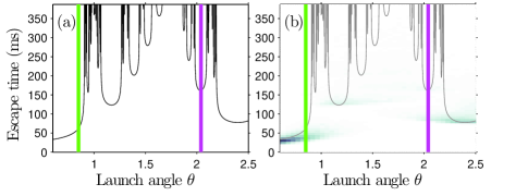
Figure 2: a) The escape-time plot. Vertical lines denote $\theta$ for the trajectories in Fig. 1b. b) The shading shows the escaping flux from an initial packet of size 500 times Planck’s constant.

Figure 2a plots the time for a trajectory with initial speed 4.12 cm/s (energy -14.9 D₂ recoils) to move from the origin to the detection line, as a function of launch angle $\theta$, measured relative to the positive $x$ axis. The resulting escape-time plot is highly singular, with numerous icicle-shaped regions whose edges tend toward infinity. These “icicles” exhibit a self-similar fractal pattern. Such patterns also occur in the chaotic ionization of hydrogen and are characteristic of chaotic escape and scattering.

A proposed experiment to measure self-similar patterns in the escape-time plot: We consider a small Gaussian packet of ultracold atoms launched from the origin with speed 4.12 cm/s and $\theta=2.04$ (the right line in Fig. 2a). The subsequent flux of atomic trajectories at the detection line is then computed as a function of time. Fig. 3a shows this flux for an initial thermal packet that occupies a phase space area 500 times Planck’s constant in both the $x$ and $y$ degrees of freedom. Fig. 3b, on the other hand, uses a packet that occupies a single Planck cell, appropriate for a pure dilute Bose-Einstein condensate (BEC) in the regime of negligible interactions. The condensate packet closely follows the trajectory in Fig. 1b, exiting as a sharp pulse at 160 ms, near the bottom of the $\theta=2.04$ icicle in Fig. 2a. The thermal packet also produces a pulse at $160$ ms, but its larger phase space extent populates neighboring icicles, thereby producing the additional pulses in Fig. 3a.

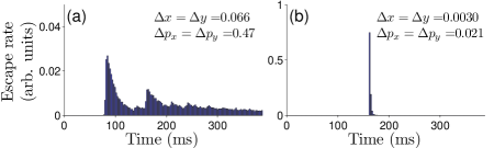
Figure 3: The flux of atoms reaching the detection line for two different Gaussian ensembles launched at $\theta=2.04$. The position and momentum widths of the initial ensembles are given in units of mm and recoil momenta ($p_{\mathrm{r}}=\hbar k_{\mathrm{\scriptscriptstyle L}}=m_{\mathrm{\scriptscriptstyle Rb}}~{}\cdot~{}5.88\;\mathrm{mm}/\mathrm{s}$ for the ⁸⁷Rb D₂ transition.)

By repeating the preceding computation for different launch angles of the thermal packet, we obtain the aggregate data in Fig. 2b, where the shading records the atomic flux as a function of arrival time and the packet’s launch angle. Fig. 3a then corresponds to the vertical slice through Fig. 2b at $\theta=2.04$. The thermal data appear as a blurred version of the sharp escape-time plot. For example, the left and right icicles are associated with prominent dark patches, and in between a few wispy patches can be associated with the bottoms of other icicles. Overall, however, the intricate icicle structure is poorly resolved by the thermal data.

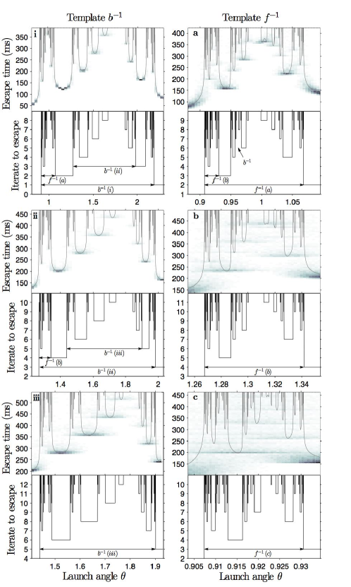
Figure 4: Escape time over six different angular intervals. Each escape-time plot is matched below by its corresponding discrete-escape-time plot.

A remarkable increase in resolution occurs below the BEC transition, shown in Fig. 4i. Many icicles are now clearly resolved, a direct consequence of the high phase-space localization afforded by the condensate. This increase in resolution prompts us to look deeper into the fractal, with the expectation that we can directly measure its fine-scale structure.

Self-similarity of the escape-time data: The first column of Fig. 4 shows data plotted for three distinct intervals of the launch angle. (We concentrate at present on the upper plot in each pair.) The three plots look remarkably similar, and icicles in one plot can be identified with icicles in the other two. In fact, this pattern of icicles occurs throughout the escape-time plot and on all scales. (See below.) One of the principal observations of this Letter is that these structures are resolved by the overlaid BEC data. The icicles look progressively more blurred as we move down the column because the interval width is decreasing and the escape time is increasing.

The pattern in the first column of Fig. 4 is not the only repeated pattern. The second column of Fig. 4 shows another pattern that also occurs on all scales throughout the same escape-time plot. As we will see, many such repeated patterns, or templates, exist in the escape-time plot. Within a given template, all other templates can be found on smaller scales. That is, each template occurs as a subtemplate of every other template in an infinitely recursive nesting. Our computations predict that several nested layers will be experimentally visible.

Experimentally, the observation of these phenomena will not be easy but certainly feasible. With a 1.06 $\mu$m laser, the above trap geometry can be realized with about 80 W of power. With this detuning, a ⁸⁷Rb atom has at most a 4% probability of spontaneous scattering over a half second. Acceleration of the atoms to the initial velocity of 4.12 $\mathrm{cm}/\mathrm{s}$ is easily accomplished; for example, a chirped, one-dimensional optical lattice of 785 nm light with 50 mW of single-beam power and beam radius $w_{0}=100\;\mu$m can accelerate the atoms in about 1.6 ms with negligible ($<1\%$) probability of spontaneous scattering and heating due to energy-band transitions. The primary difficulty is the subrecoil initial conditions required, even in the thermal case. However, a standard expanded BEC should suffice.

Theoretical foundations of the fractal structure: We next describe how the self-similar fractal data can be described with recently developed symbolic tools Mitchell06 . We first specify a two-dimensional surface of section in the $xyp_{x}p_{y}$-phase space by fixing the energy $E$ at -14.9 D₂ recoils and setting $y=0$. Thus, every time a trajectory passes through the $x$-axis, we can record $(x,p_{x})$, defining a Poincaré map that maps a given intersection $(x,p_{x})$ forward to the next intersection $(x^{\prime},p_{x}^{\prime})$. Fig. 5 shows the corresponding surface-of-section plot. The vertical line $\mathcal{L}_{0}$ at $x=0$ consists of all points at the origin moving outward with arbitrary launch angle $\theta$. The point $\mathbf{z}_{\mathsf{X}}$ is the unstable fixed point equal to the intersection of the unstable periodic orbit (PO) in Fig. 1b with the surface of section. Attached to $\mathbf{z}_{\mathsf{X}}$ are its stable $\mathcal{S}$ (thick) and unstable $\mathcal{U}$ (thin) manifolds, consisting of all points that asymptote to $\mathbf{z}_{\mathsf{X}}$ in the forward and backward directions, respectively. These manifolds intersect an infinite number of times, forming an intricate pattern called a homoclinic tangle Wiggins92 ; Mitchell06 ; tangles ; Mitchell03 . The segments of the stable and unstable manifolds connecting $\mathbf{z}_{\mathsf{X}}$ to the point $\mathbf{P}_{0}$ define the shaded region called the “complex”.

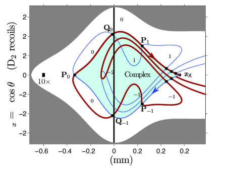
Figure 5: The surface of section, showing the unstable fixed point $\mathbf{z}_{\mathsf{X}}$ and its associated homoclinic tangle. The left rectangle has area ten times Planck’s constant.

Escape from the complex occurs via escape lobes $E_{n}$, defined in Fig. 5 as the regions bounded by the stable and unstable segments connecting $\mathbf{P}_{n}$ to $\mathbf{Q}_{n}$. The lobe $E_{-1}$, inside the complex, maps to $E_{0}$, outside the complex. Once in $E_{0}$ a point then maps to $E_{1}$, $E_{2}$, etc., eventually passing into the secondary well on the right. The lobes $E_{-k}$ contain all points that escape in $k$ iterates. These lobes become progressively more stretched and folded as $k$ increases. (An analogous sequence of lobes $C_{n}$ controls capture into the complex.) Note that we are able to chose physical parameters that make the lobes quite large compared to Planck’s constant (Fig. 5).

We plot as a function of $\theta$ the number of iterates for a point to escape the complex, shown as the lower plot of each pair in Fig. 4. These plots straighten each icicle into a constant escape segment. A segment that escapes on iterate $k$ is an intersection between $E_{-k}$ and $\mathcal{L}_{0}$. For example, the segment at iterate two in Fig. 4i is the intersection with $E_{-2}$ in Fig. 5.

Ref. Mitchell06 introduces a symbolic technique, called homotopic lobe dynamics, to compute the structure of escape segments based on the tangle topology. (See also Refs. tangles .) We summarize the results obtained from applying this technique to the tangle in Fig. 5.

The structure of the discrete-escape-time plot up to a given iterate $n$ is specified by a string $\ell_{n}$ of symbols in the set $\{c_{1},c_{2},a,b,f,u_{0},u_{1},u_{2},...\}$ as well as their inverses, e.g. $c_{1}^{-1}$. The first string is $\ell_{1}=u_{1}b^{-1}u_{0}$. All subsequent strings can be obtained from the first by mapping each symbol forward according to the substitution rules:

$$c_{1} \mapsto c_{2}, c_{2} \mapsto f^{-1}u_{0}au_{0}^{-1}f,$$ (2a)

$$a \mapsto b^{-1}u_{0}^{-1}b, f \mapsto c_{1}^{-1}u_{0}^{-1}f,$$ (2b)

$$u_{n} \mapsto u_{n+1}, b \mapsto b^{-1}u_{0}^{-1}f,$$ (2c)

using the standard convention for iterating inverses, e.g. $b^{-1}\mapsto f^{-1}u_{0}b$. For example, the first four strings are:

$$\ell_{1} =u_{1}b^{-1}\underline{u_{0}},$$ (3a)

$$\ell_{2} =u_{2}f^{-1}\underline{u_{0}}bu_{1},$$ (3b)

$$\ell_{3} =u_{3}f^{-1}\underline{u_{0}}c_{1}u_{1}b^{-1}\underline{u_{0}^{-1}}fu_{2},$$ (3c)

$$\ell_{4} =u_{4}f^{-1}\underline{u_{0}}c_{1}u_{1}c_{2}u_{2}f^{-1}\underline{u_{0}}bu_{1}^{-1}c_{1}^{-1}\underline{u_{0}^{-1}}fu_{3}.$$ (3d)

An $\ell_{n}$ string encodes the discrete-escape-time plot as follows. Each appearance of $u_{0}^{\pm 1}$ in $\ell_{n}$ (underlined for emphasis) represents a segment that escapes at iterate $n$. For example, the $u_{0}$ factor in Eq. (3a) corresponds to the escape segment at iterate one in Fig. 4i. This $u_{0}$ factor then maps forward to $u_{1}$ in Eq. (3b). In general, we see that each $u_{k}^{\pm 1}$ in $\ell_{n}$ represents a segment that escapes at iterate $n-k$. In Eq. (3b), another $u_{0}$ factor has appeared, corresponding to the escape segment at iterate two. This segment is to the left of the first segment, just as the $u_{0}$ factor in Eq. (3b) is to the left of the $u_{1}$ factor. In general, the left-right ordering of $u_{k}^{\pm 1}$ symbols in $\ell_{n}$ represents the left-right ordering of segments in the discrete-escape-time plot. On the next two iterates, two new $u_{0}$ factors appear in Eq. (3c), and three more appear in Eq. (3d), in agreement with Fig. 4i.

All other symbols besides $u_{k}^{\pm 1}$ represent gaps between adjacent escape segments. For example, $b^{-1}$ in Eq. (3a) represents the gap $b^{-1}(i)$ in Fig. 4i, and $b^{-1}$ in Eq. (3c) represents the gap $b^{-1}(ii)$ in Figs. 4i and  4ii. The string $\ell_{5}$ will also contain a $b^{-1}$ factor, representing the gap $b^{-1}(iii)$ in Figs. 4ii and 4iii. Since each $b^{-1}$ factor generates exactly the same string of symbols under Eqs. (2), each gap labeled $b^{-1}$ in Fig. 4 contains the same pattern of escape segments. This means that $b^{-1}$ corresponds to a particular template, i.e. to find occurrences of this template in the escape-time plot, we need only look for occurrences of $b^{-1}$ in the expression for $\ell_{n}$.

It follows from the above logic that each symbol $\{c_{1},c_{2},a,b,f\}$ generates its own template, with inverse symbols generating reflected templates. For example, mapping $f^{-1}$ forward three times yields

$$f^{-1}u_{0}c_{1}u_{1}c_{2}u_{2}f^{-1}u_{0}au_{0}^{-1}f.$$ (4)

The reader may verify that Eq. (4) describes the segments up to iterates five, seven, and six in Figs. 4a, 4b, and 4c. Note that different experimental parameters will yield different algebraic rules and different templates.

This algebraic formalism computes a minimal set of escape segments, but generally not all segments. That is, at later times, we typically find additional segments in the numerics. This illustrates what has previously been called an epistrophic fractal Mitchell03 . Nevertheless, unpredicted segments can be accommodated within an updated algebraic formalism, as explained in Ref. Mitchell06 .

Conclusions: We predict that experiments on the intermediate-time escape dynamics of ultracold atoms from an optical trap can directly image fractals. The resolution is particularly good when using a BEC. The fractal structure depends on the topology of homoclinic tangles, which are common to numerous chaotic systems. Such experiments would thus provide a new laboratory tool for the study of an important chaotic mechanism. Similarly, an improved understanding of the chaotic escape pathways of atoms from optical traps could be relevant for the understanding of mixing and thermalization in traps and for the control and coherent emission of atomic wavepackets. Finally, the dependence of these fractals on atom density could serve as an interesting probe of atom-atom interactions, a subject to be explored in future work.

References

- (1) R. Taylor et al., in Electron Transport in Quantum Dots, J. P. Bird ed. (Kluwer, Dordrecht, 2003).
- (2) C. Gmachl et al., Science 280, 1556 (1998).
- (3) M. J. Davis and S. K. Gray, J. Chem. Phys. 84, 5389 (1986); M. J. Davis and R. E. Wyatt, Chem. Phys. Lett. 86, 235 (1982); A. Tiyapan and C. Jaffé, J. Chem. Phys. 99, 2765 (1993); 101, 10393 (1994); 103, 5499 (1995); F. Gabern et al., Physica D 211, 391 (2005); T. Uzer et al., Nonlinearity 15, 957 (2002).
- (4) W. S. Koon et al., Chaos 10, 427 (2000); C. Jaffé et al., Phys. Rev. Lett. 89, 011101 (2002).
- (5) R. V. Jensen, S. M. Susskind, and M. M. Sanders, Phys. Rep. 201, 1 (1991); P. M. Koch and K. A. H. van Leeuwen, Phys. Rep. 255, 289 (1995).
- (6) K. A. Mitchell et al., Phys. Rev. Lett. 92, 073001 (2004); Phys. Rev. A 70, 043407 (2004).
- (7) T. Topcu and F. Robicheaux (private communication).
- (8) S. Wiggins, Chaotic Transport in Dynamical Systems (Springer-Verlag, New York, 1992).
- (9) V. Milner et al., Phys. Rev. Lett. 86, 1514 (2001).
- (10) N. Friedman et al., Phys. Rev. Lett. 86, 1518 (2001).
- (11) K. A. Mitchell and J. B. Delos, Physica D 221, 170 (2006).
- (12) R. W. Easton, Trans. Am. Math. Soc. 294, 719 (1986); V. Rom-Kedar, Physica D 43, 229 (1990); V. Rom-Kedar, Nonlinearity 7, 441 (1994); B. Rückerl and C. Jung, J. Phys. A 27, 6741 (1994); C. Lipp and C. Jung, J. Phys. A 28, 6887 (1995); C. Jung and A. Emmanouilidou, Chaos 15, 023101 (2005); P. Collins, Internat. J. Bifur. Chaos Appl. Sci. Engrg. 12, 605 (2002); P. Collins, Dyn. Syst. 19, 1 (2004); P. Collins, Dyn. Syst. 20, 369 (2005); P. Collins, Experiment. Math. 14, 75 (2005).
- (13) K. A. Mitchell et al., Chaos 13, 880 (2003); K. A. Mitchell et al., Chaos 13, 892 (2003).