Intra-cellular transport by single-headed kinesin KIF1A: effects of single-motor mechano-chemistry and steric interactions

Abstract

In eukaryotic cells, many motor proteins can move simultaneously on a single microtubule track. This leads to interesting collective phenomena like jamming. Recently we reported (Phys. Rev. Lett. 95, 118101 (2005)) a lattice-gas model which describes traffic of unconventional (single-headed) kinesins KIF1A. Here we generalize this model, introducing a novel interaction parameter $c$, to account for an interesting mechano-chemical process which has not been considered in any earlier model. We have been able to extract all the parameters of the model, except $c$, from experimentally measured quantities. In contrast to earlier models of intra-cellular molecular motor traffic, our model assigns distinct “chemical” (or, conformational) states to each kinesin to account for the hydrolysis of ATP, the chemical fuel of the motor. Our model makes experimentally testable theoretical predictions. We determine the phase diagram of the model in planes spanned by experimentally controllable parameters, namely, the concentrations of kinesins and ATP. Furthermore, the phase-separated regime is studied in some detail using analytical methods and simulations to determine e.g. the position of shocks. Comparison of our theoretical predictions with experimental results is expected to elucidate the nature of the mechano-chemical process captured by the parameter $c$.

I Introduction

Motor proteins are responsible for intra-cellular transport of wide varieties of cargo from one location to another in eukaryotic cells schliwa ; molloy ; jphys . One crucial feature of these motors is that these move on filamentary tracks polrev . Microtubules and filamentary actin are protein filaments which form part of a dual-purpose scaffolding called cytoskeleton howard ; these filamentary proteins act like struts or girders for the cellular architecture and, at the same time, also serve as tracks for the intra-cellular transportation networks. Kinesins and dyneins are two superfamilies of motors that move on microtubule whereas myosins move on actin filaments. A common feature of all these molecular motors is that these perform mechanical work by converting some other form of input energy. However, there are several crucial differences between these molecular motors and their macroscopic counterparts; the major differences arise from their negligibly small inertia. That’s why the mechanisms of single molecular motors schliwa ; molloy ; jphys and the details of the underlying mechano-chemistry bustamante have been investigated extensively over the last two decades.

However, often a single filamentary track is used simultaneously by many motors and, in such circumstances, the inter-motor interactions cannot be ignored. Fundamental understanding of these collective physical phenomena may also expose the causes of motor-related diseases (e.g., Alzheimer’s disease) traffd thereby helping, possibly, also in their control and cure.

To our knowledge, the first attempt to understand effects of steric interactions of motors was made in the context of ribosome traffic on a single mRNA strand macdonald . This led to the model which is now generally referred to as the totally asymmetric simple exclusion process (TASEP); this is one of the simplest models of non-equilibrium systems of interacting driven particles sz ; derrida ; schuetz . In the TASEP a particle can hop forward to the next lattice site, with a probability $q$ per time step, if and only if the target site is empty; updating is done throughout either in parallel or in the random-sequential manner.

Some of the most recent generic theoretical models of interacting cytoskeletal molecular motors lipo ; frey1 ; santen ; popkov are appropriate extensions of TASEP. In those models the motor is represented by a self-driven particle and the dynamics of the model is essentially an extension of that of the TASEP sz ; schuetz that includes Langmuir-like kinetics of attachment and detachment of the motors. Two different approaches have been suggested. In the approach followed by Parmeggiani, Franosch and Frey (PFF model) frey1 ; frey2 , attachment and detachment of the motors is modelled, effectively, as particle creation and annihilation, respectively, on the track; the diffusive motion of the motors in the surrounding fluid medium is not described explicitly. In contrast, in the alternative formulation suggested by Lipowsky and co-workers lipo ; lipo2 , the diffusion of motors in the cell is also modelled explicitly.

In reality, a motor protein is not a mere particle, but an enzyme whose mechanical movement is coupled with its biochemical cycle. In a recent letter nosc we considered specifically the single-headed kinesin motor, KIF1A okada1 ; okada2 ; okada3 ; okada4 ; okada5 . The movement of a single KIF1A motor had already been modelled earlier okada2 ; sasaki by a Brownian ratchet mechanism julicher ; reimann . In contrast to the earlier models lipo ; frey1 ; santen ; popkov of molecular motor traffic, which take into account only the mutual interactions of the motors, our model explicitly incorporates also this Brownian ratchet mechanism of the individual KIF1A motors, including its biochemical cycle that involves adenosine triphosphate (ATP) hydrolysis.

The TASEP-like models predict the occurrence of shocks. But since most of the bio-chemistry is captured in these models through a single effective hopping rate, it is difficult to make direct quantitative comparison with experimental data which depend on such chemical processes. In contrast, the model we proposed in ref. nosc incorporates the essential steps in the biochemical processes of KIF1A as well as their mutual interactions and involves parameters that have one-to-one correspondence with experimentally controllable quantities.

Here, we present not only more details of our earlier calculations but also many new results on the properties of single KIF1A motors as well as their collective spatio-temporal organization. Moreover, here we also generalize our model to account for a novel mechano-chemical process which has not received any attention so far in the literature. More specifically, two extreme limits of this generalized version of the model correspond to two different plausible scenarios of ADP release by the motor enzymes. To our knowledge okadapc , at present, it is not possible to rule out either of these two scenarios on the basis of the available empirical data. However, our new generalized model helps in prescribing clear quantitative indicators of these two mutually exclusive scenarios; use of these indicators in future experiments may help in identifying the true scenario.

An important feature of the collective spatio-temporal organization of motors is the occurance of a shock or domain wall, which is essentially the interface between the low-density and high-density regions. We focus on the dependence of the position of the domain wall on the experimentally controllable parameters of the model. Moreover, we make comparisons between our model in the low-density regime with some earlier models of single motors. We also compare and contrast the basic features of the collective organization in our model with those observed in the earlier generic models of molecular motor traffic.

II Discretized Brownian ratchet model for KIF1A: general formulation

Through a series of in-vitro experiments, Okada, Hirokawa and co-workers established okada1 ; okada2 ; okada3 ; okada4 ; okada5 that:

1. KIF1A molecule is an enzyme (catalyst) and in each enzymatic cycle it hydrolyzes one ATP molecule; the products of hydrolysis being adenosine diphosphate (ADP) and inorganic phosphate. Thus, each biochemical cycle of a KIF1A motor consists of four states: bare kinesin (K), kinesin bound with ATP (KT), kinesin bound with ADP and phosphate (KDP) and, finally, kinesin bound with only ADP (KD) after releasing phosphate (Fig. 1).

2. When a single-headed kinesin binds with a ATP molecule, its binding with its microtubule track is weakened by the ATP hydrolysis. Both K and KT bind strongly to microtubules. Hydrolysis of ATP leads to the state KDP which has a very short lifetime and soon yields KD by releasing phosphate. KD binds weakly to a microtubule. After releasing all the products of hydrolysis (i.e., ADP and phosphate), the motor again binds strongly with the nearest binding site on the microtubule and thereby returns to the state K.

3. In the state KD, the motor remains tethered to the microtubule filament by the electrostatic attraction between the positively charged $K$-loop of the motor and the negatively charged $E$-hook of the microtubule filament. Because of this tethering in the weakly bound state, a KIF1A cannot wander far away from the microtubule, but can execute (essentially one-dimensional) diffusive motion parallel to the microtubule filament. However, in the strongly bound state, the KIF1A motor cannot execute diffusive excursions away from the binding site on the microtubule.

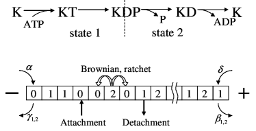
Figure 1: A biochemical cycle of a KIF1A motor (upper) and a three-valued discrete model for traffic of interacting KIF1A motors on a finite microtubule filament (lower). The states left to the dotted line in the upper figure correspond to strongly bound to microtubule states (state 1) while those right are weakly bound (state 2). 0 denotes an empty site, and only 2 can move either to the forward or backward site. Transition from 1 to 2 occurs at the same site which corresponds hydrolysis, and the detachment also happens in this process. The attachment is possible only at the empty sites. At the minus and plus ends the probabilities are different from those at sites in the bulk.

These experimental results for the biochemical cycle of KIF1A motors indicate that a simplified description in terms of a 2-state model could be sufficient to understand the collective transport properties. As shown in Fig. 1 one distinguishes a state where the motor is strongly bound to the microtubule (state 1) and a state where it is weakly bound (state 2). It is worth pointing out that such a simplified 2-state model, however, may not be adequate to capture the biochemical cycle of other motors like, for example, conventional kinesins. In such situations, a more detailed 4-state model is required.

As in the TASEP-type approach of the PFF model, the periodic array of the binding sites for KIF1A on the microtubule are represented as a one-dimensional lattice of sites that are labelled by the integer index $i$ ($i=1,...,L$). KIF1A motors are represented by particles that can be in two different states 1 and 2, corresponding to the strongly-bound and weakly bound states. To account for the empirical observations, the model also contains elements of a Brownian ratchet. As in the PFF model, attachment and detachment of a motor are modelled as, effectively, creation and annihilation of the particles on the lattice. We use the random sequential update, and the dynamics of the system is given by the following rules of time evolution:

(1) Bulk dynamics
If the chosen site on the microtubule is empty, i.e., in state $0$, then with probability $\omega_{a}dt$ a motor binds with the site causing a transition of the state of the binding site from $0$ to $1$. However, if the binding site is in state $1$, then it becomes $2$ with the probability $\omega_{h}dt$ due to hydrolysis, or becomes $0$ with probability $\omega_{d}dt$ due to the detachment from the microtubule during hydrolysis.

If the chosen site is in state $2$, then the motor bound to this site steps forward to the next binding site in front by a ratchet mechanism with the rate $\omega_{f}$ or stays at the current location with the rate $\omega_{s}$. Both processes are triggered by the release of ADP. How should one modify these update rules if the next binding site in front is already occupied by another motor? Does the release of ADP from the motor, and its subsequent re-binding with the filamentary track, depend on the state of occupation of the next binding site in front of it? To our knowledge, experimental data available at present in the literature are inadequate to answer this question. Nevertheless, we can think of the two following plausible scenarios: in the cases $\cdots 21\cdots$, or $\cdots 22\cdots$, the following kinesin, which is in state 2, can return to state 1, only at its current location, with rate $\omega_{s}$ if ADP release is regulated by the motor at the next site in front of it. But, if ADP release by the kinesin is independent of the occupation status of the front site, then state 2 can return to state 1 at the fixed rate $\omega_{s}+\omega_{f}$, irrespective of whether or not the front site is occupied.

Therefore, we propose a generalization of our original model by incorporating both these possible scenarios within a single model by introducing an interpolating parameter $c$ with $0\leq c\leq 1$. In this generalized version of our model, a motor in the state 2 returns to the state 1 at the rate $\omega_{s}+(1-c)\omega_{f}$. The parameter $c$ $(0\leq c\leq 1)$ allows interpolation between the two above mentioned scenarios of ADP release by the kinesin. For $c=1$ the transition from the strongly to the weakly bound state in the ratchet mechanism depends on the occupation of the front site. This is the case that has been treated in nosc , where the release of ADP by a nucleotide-bound kinesin is tightly controlled by the kinesin at the next binding site in front of it. On the other hand, for $c<1$ the transition rate will depend partially on the occupation of the front site. For $c=0$ the ADP release process becomes completely independent of the state of the preceeding site.

As long as the motor does not release ADP, it executes random Brownian motion with the rate $\omega_{b}$.

(2) Dynamics at the ends
The probabilities of detachment and attachment at the two ends of the microtubule can be different from those at any other site in the bulk. We choose $\alpha$ and $\delta$, instead of $\omega_{a}$, as the probabilities of attachment at the left and right ends. Similarly, we take $\gamma_{1}$ and $\beta_{1}$, instead of $\omega_{d}$, as probabilities of detachments at the left and right ends, respectively (Fig. 1). Finally, $\gamma_{2}$ and $\beta_{2}$, instead of $\omega_{b}$, are the probabilities of exit of the motors through the two ends by random Brownian movements.

For the dynamical evolution of the system, one of the $L$ sites is picked up randomly and updated according to the rules given below together with the corresponding probabilities (Fig. 2):

$${\rm Attachment:}\,\,\,\,\,0\to 1\,\,\,{\rm with}\,\,\omega_{a}dt$$ (1)

$${\rm Detachment:}\,\,\,\,1\to 0\,\,\,{\rm with}\,\,\omega_{d}dt$$ (2)

$${\rm Hydrolysis:}\,\,\,\,\,\,1\to 2\,\,\,{\rm with}\,\,\omega_{h}dt$$ (3)

$${\rm Brownian\ motion:}\,\,\,\,\,\left\{\begin{array}[]{c}20\to 02\,\,\,{\rm with}\,\,\omega_{b}dt\\ 02\to 20\,\,\,{\rm with}\,\,\omega_{b}dt\end{array}\right.$$ (6)

$${\rm Ratchet:}\,\,\,\,\left\{\begin{array}[]{l}20\to 10\,\,\,\,\,{\rm with}\,\,\omega_{s}dt\\ 2X\to 1X\,\,\,{\rm with}\,\,\left(\omega_{s}+(1-c)\omega_{f}\right)dt\\ 20\to 01\,\,\,\,\,{\rm with}\,\,\omega_{f}dt\end{array}\right.$$ (10)

Here $X$ denotes an occupied site irrespective of the chemical state of the motor, i.e., a site occupied by a motor that is in either state 1 or state 2.

The ratchet mechanism (10) is triggered by the release of ADP and summarizes the transitions of a particle from state 2 to state 1. It distinguishes the two initial states $20$, where the front site is empty, and $2X$, where the front site is occupied. We see that the overall transition rate from state 2 to state 1 is $\omega_{s}+\omega_{f}$ if the front site is empty (initial state $20$), and it is $\omega_{s}+(1-c)\omega_{f}$ if the front site is occupied (initial state $2X$). This reflects the dependence of the ADP release rate on the front site occupation whenever $c\neq 0$.

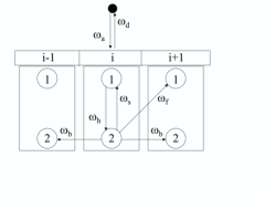
Figure 2: Schematic description of the three-state model of a single-headed kinesin motor that follows a Brownian ratchet mechanism. In the special case $2X\to 1X$, which has not been shown explicitly for the sake of simplicity, the rate constants would get modified following the prescriptions described in the text.

The physical processes captured by the rate constants $\omega_{f}$ and $\omega_{s}$ can be understood as follows by analyzing the Brownian ratchet mechanism illustrated in Fig. 3.

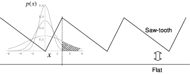
Figure 3: The two forms of the time-dependent potential used for implementing the Brownian ratchet mechanism.

For the sake of simplicity, we consider only one molecular motor, and let us imagine that the potential seen by the motor periodically oscillates between the sawtooth shape and the flat shape shown in Fig. 3. When the sawtooth form remains “on” for some time, the particle settles at the bottom of a well. Then, when the potential is switched “off”, the probability distribution of the position of the particle is given by a delta function which, because of free diffusion in the absence of any force, begins to spread. After some time the Gaussian profile spreads to such an extent that it has some overlap also with the well in front, in addition to the overlap it has with the original well. At that stage, when the sawtooth potential is again switched on, there is a non-vanishing probability that the particle will find itself in the well in front; this probability is proportional to the area of the hatched part of the Gaussian profile shown in Fig. 3 and is accounted for in our model by the parameter $\omega_{f}$. There is also significant probability that the particle will fall back into the original well; this is captured in our model by the parameter $\omega_{s}$.

II.1 Parameters of the model

From experimental data okada1 ; okada3 , good estimates for the parameters of the suggested model can be obtained. The detachment rate $\omega_{d}\simeq 0.1$ s^-1 is found to be independent of the kinesin population. On the other hand, $\omega_{a}=10^{7}$ $C$/M$\cdot$s depends on the concentration $C$ (in M) of the kinesin motors. In typical eucaryotic cells in-vivo the kinesin concentration can vary between $10$ and $1000$ nM. Therefore, the allowed range of $\omega_{a}$ is $0.1$ s${}^{-1}\leq\omega_{a}\leq 10$ s^-1.

Total time taken for the hydrolysis of one ATP molecule is about $9$ ms of which $4$ ms is spent in the state $1$ and $5$ ms in the state $2$. The corresponding rates $1/4$ and $1/5$ are shown in Fig. 4. The motion of KIF1A is purely diffusive only when it is in the state $2$ and the corresponding diffusion coefficient is denoted by the symbol $D_{2}$. Using the measured diffusion constant $D=40,000$ nm²/s okada2 and the relation $D_{2}=(9/5)D$, we get $D_{2}=72,000$ nm²/s (see Fig. 4(b)). The time $\omega_{b}^{-1}$ must be such that $\omega_{b}\sim D_{2}/(8\text{nm})^{2}$, and, hence, we get $\omega_{b}\simeq 1125$ s^-1.

Moreover, from the experimental observations that the mean step size is $3$ nm whereas the separation between the successive binding sites on a microtubule is $8$ nm, we conclude $\omega_{f}/\omega_{s}\simeq 3/8$. Furthermore, from the measured total time of each cycle, we estimate that $\omega_{s}+\omega_{f}\simeq 200$ s^-1. From these two relations between $\omega_{f}$ and $\omega_{s}$ we get the individual estimates $\omega_{s}\simeq 145$ s^-1 and $\omega_{f}\simeq 55$ s^-1.

Assuming the validity of the Michaelis-Menten type kinetics for the hydrolysis of ATP howard , the experimental data suggest that

$$\frac{1}{V}=\frac{1}{V_{max}}\biggl{(}1+\frac{K_{m}}{[ATP]}\biggr{)}$$ (11)

where $[ATP]$ is the ATP concentration (in mM), $K_{m}$ is the Michaelis constant given by $K_{m}=0.1$ mM in this case. $V$ and $V_{max}$ (in ms^-1) are the reaction rate and its maximum value respectively. As mentioned earlier $1/V_{max}\simeq 9$ ms. Since $1/V=\omega_{h}^{-1}+5$ ms, we finally get

$$\omega_{h}^{-1}\simeq\biggl{[}4+9\biggl{(}\frac{0.1~{}\text{mM}}{\text{ATP concentration (in mM)}}\biggr{)}\biggr{]}\text{ms}$$ (12)

so that the allowed biologically relevant range of $\omega_{h}$ is $0\leq\omega_{h}\leq 250$ s^-1.

Up to now, experimental investigations could not determine the parameter $c$. We therefore treat it as a free parameter in the following to study the effects that it has on the phase diagram, position of shocks etc. Comparison with empirical results then might help to get an estimate for $c$.

Figure 4: The biochemical cycle of KIF1A is shown to define some important parameters which can be extracted from experimental data. See text for more details.

II.2 Mean-field equations

Let us denote the probabilities of finding a KIF1A molecule in the states $1$ and $2$ at the lattice site $i$ at time $t$ by the symbols $S_{i}$ and $W_{i}$, respectively. In mean-field approximation, the master equations for the dynamics of the interacting KIF1A motors in the bulk of the system are given by

$$\frac{dS_{i}}{dt} = \omega_{a}(1-S_{i}-W_{i})-\omega_{h}S_{i}-\omega_{d}S_{i}$$ (13)

$$+\omega_{s}W_{i}+\omega_{f}W_{i-1}(1-S_{i}-W_{i})$$

$$+(1-c)\,\omega_{f}W_{i}(S_{i+1}+W_{i+1}),$$

$$\frac{dW_{i}}{dt} = -(\omega_{s}+\omega_{f})W_{i}(1-S_{i+1}-W_{i+1})+\omega_{h}S_{i}$$ (14)

$$-(\omega_{s}+(1-c)\omega_{f})W_{i}(S_{i+1}+W_{i+1})$$

$$-\omega_{b}W_{i}(2-S_{i+1}-W_{i+1}-S_{i-1}-W_{i-1})$$

$$+\omega_{b}(W_{i-1}+W_{i+1})(1-S_{i}-W_{i})$$

$$= -(\omega_{s}+\omega_{f})W_{i}+\omega_{h}S_{i}+c\,\omega_{f}W_{i}(S_{i+1}+W_{i+1})$$

$$-\omega_{b}W_{i}(2-S_{i+1}-W_{i+1}-S_{i-1}-W_{i-1})$$

$$+\omega_{b}(W_{i-1}+W_{i+1})(1-S_{i}-W_{i}).$$

The corresponding equations for the left boundary ($i=1$) are given by

$$\frac{dS_{1}}{dt} = \alpha(1-S_{1}-W_{1})+\omega_{s}W_{1}-\omega_{h}S_{1}-\gamma_{1}S_{1}$$ (15)

$$+(1-c)\omega_{f}W_{1}(S_{2}+W_{2}),$$

$$\frac{dW_{1}}{dt} = \omega_{h}S_{1}-(\omega_{s}+\omega_{f})W_{1}+c\omega_{f}W_{1}(S_{2}+W_{2})$$ (16)

$$-\gamma_{2}W_{1}+\omega_{b}W_{2}(1-S_{1}-W_{1})$$

$$-\omega_{b}W_{1}(1-S_{2}-W_{2}),$$

while those for the right boundary ($i=L$) are given by

$$\frac{dS_{L}}{dt} = \delta(1-S_{L}-W_{L})+\omega_{f}W_{L-1}(1-S_{L}-W_{L})$$ (17)

$$+\omega_{s}W_{L}-\omega_{h}S_{L}-\beta_{1}S_{L},$$

$$\frac{dW_{L}}{dt} = \omega_{h}S_{L}-\omega_{s}W_{L}-\beta_{2}W_{L}$$ (18)

$$+\omega_{b}W_{L-1}(1-S_{L}-W_{L})$$

$$-\omega_{b}W_{L}(1-S_{L-1}-W_{L-1}).$$

In the following we shall determine solutions of this set of equations for several cases and compare with the corresponding numerical results from computer simulations.

III Comparison with other models for motor traffic

In this section we compare our model with earlier models of molecular motor traffic. The first two subsections describe models developed for non-interacting molecular motors whereas in the last subsection we collect the main results for the PFF model which has been introduced to study collective effects in motor traffic. A more detailed comparison with models of interacting motors will be taken up later in section V of this paper.

Chen chen developed a model for single-headed kinesins assuming a power stroke mechanism. He assumed that each kinesin can attain three distinct states which were labelled by the symbols $0$, $1$ and $2$. The kinesin was assumed to be detached from the microtubule in the state $0$, but bound to microtubule in the other two states. The states $1$ and $2$ were assumed to differ from each other by the amount of their tilt in the direction of motion. The molecule steps ahead by exactly $8$ nm in one cycle consuming one ATP molecule. This power-stroke model fails to account for several aspects of experimental data (for example, the distribution of the steps sizes, including backward steps) on KIF1A and, therefore, will not be considered further for quantitative comparison.

III.1 Comparison with Sasaki’s Brownian ratchet model

In contrast to the power-stroke model developed by Chen chen , Sasaki sasaki quantified the Brownian-ratchet model for a single KIF1A motor proposed by Okada and Hirokawa okada1 ; okada2 . He used the standard Fokker-Planck approach julicher ; reimann . In this formulation, the particle, which represents a kinesin, is assumed to be subjected to a time-dependent periodic potential as given in Fig. 3. The potential switches from one shape $V_{1}(x)$ to another shape $V_{2}(x)$ with rate $\omega_{1}$ and the reverse switching takes place at a rate $\omega_{2}$. One of the shapes of this potential $V_{1}(x)$ is taken to be a periodic repetition of a saw-tooth where each saw-tooth itself is asymmetric. Suppose, the height of the maximum of each sawtooth is $U$. The shape of the form of the potential $V_{2}(x)$ was assumed to be flat, i.e., $V_{2}(x)=0$ for all $x$. Sasaki calculated the average speed $v$ and the diffusion coefficient $D$ as functions of $U$, $\omega_{1}$ and $\omega_{2}$.

One advantage of our model over Sasaki’s model is that we do not make any ad-hoc assumption regarding the shape of the potential as the potential does not enter explicitly into our formulation. It is possible to identify $\omega_{1}$ in Sasaki’s model with $\omega_{h}$ in our model. The rate constant $\omega_{2}$ can be related to the rates in our model in the following way: $\omega_{2}=\omega_{s}+\omega_{f}$ if the preceding site is unoccupied and $\omega_{2}=\omega_{s}+(1-c)\omega_{f}$ if it is occupied.

III.2 Comparison with Fisher-Kolomeisky multi-step chemical kinetic model

Next we make a comparison between our model and the multi-step chemical kinetic approach developed by Fisher and Kolomeisky kolo1 ; kolo2 ; kolo3 for molecular motors. In the simplest case of a single filament, the equispaced binding sites on a microtubule are assumed to form a one-dimensional lattice. It is assumed that there are $M$ distinct discrete intermediate chemical states on a biochemical pathway between two consecutive binding sites. The motor in state $j_{i}$ (i.e., in chemical state $j$ located at spatial position $i$ where $1\leq j\leq M$, $1\leq i\leq L$) can make transitions to the states $(j+1)_{i}$ and $(j-1)_{i}$ with the rates $u_{j}$ and $w_{j}$, respectively (see Fig. 5). Note that we have labelled the chemical states in such a way that $M_{i}=1_{i+1}$ ($M_{i}=2$ in Fig. 5) such that, completion of the chain in forward (backward) transitions through these $M$ states would translocate the motor forward (backward) by one lattice spacing.

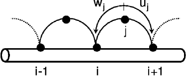
Figure 5: Fisher-Kolomeisky multi-step chemical kinetic model of molecular motors.

Clearly, in the absence of attachment and detachment of the motors, our model for a single KIF1A reduces to the Fisher-Kolomeisky multi-step chemical kinetic model of molecular motors on a single filament (see Fig.6) where $M=2$, as emphasized by a slight redrawing of our model in Fig. 6.

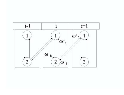
Figure 6: In the absence of attachment and detachment, our model is equivalent to Fisher-Kolomeisky model shown in Fig. 5.

Direct quantitative comparison with our model is also possible. For example, in the special case where only forward transitions are allowed and $M=2$, the average speed of the motor in the Fisher-Kolomeisky model is given by

$$v=\frac{u_{1}u_{2}}{u_{1}+u_{2}}$$ (19)

where distance is measured in the units of spacing between two successive binding sites ($8$ nm in case of microtubule). In Sec. IV.2 we will derive an analogous expression for our model, see (24).

III.3 Comparison with PFF-model

The Parmeggiani-Franosch-Frey model (PFF model) frey1 combines the TASEP with Langmuir kinetics. The motors are assumed to step forward one site with rate $p$ if the front site is empty, but do not move if this site is occupied (exclusion). A backwards movement is not possible. In addition, motors can attach to empty sites with rate $\omega_{a}$ and detach from a site with rate $\omega_{d}$. This might be the simpliest model for intracellular transport including adsorption and desorption. Although quite basic, it already reproduces the qualitative behavior of a large class of many-motor systems. It not only shows high-, low- and maximum-current phases like TASEP, but also phase coexistence for distinct parameter ranges, while phase domains are separated by stationary domain walls (shocks). These shocks are also observed in experiments nosc . Shock phases appear if the Langmuir kinetics are of the same order as motor attachment and detachment at the ends. It means that in the continious limit where system size $L\to\infty$, the local attachment and detachment rates $\omega_{a}$ and $\omega_{d}$ have to be rescaled so that the global attachment and detachment rates defined as $\Omega_{a}:=\omega_{a}L,\,\,\Omega_{d}:=\omega_{d}L$ stay constant. One can argue that the topology of the phase diagram of the PFF model is quite universal for systems that, as the PFF model, possess a current-density relation with one single maximum and the same Langmuir kinetics popkov , so even more complex models might show similiar qualitative behavior as the PFF model.

Although the PFF model reproduces qualitative properties of intracellular transport quite well, it is difficult to associate the hopping parameter $p$ quantitatively with experimentally accessible biochemical quantities because the biochemical processes of a motor making one step are usually quite complex. The PFF model does not take into account these processes. Furthermore, it is not possible to include interactions in the PFF model that only influence particular transitions of the biochemical states of the motor. The advantage of our model is the possibility of calibration of the model parameters with experimentally controllable parameters ATP- or motor protein concentration. Through the parameter $c$ we can include, at least phenomenologically, an interaction that controls the transition from one state (2) to another (1).

IV Single motor properties and calibration

In this section we first investigate the dynamics of our model in the limit of vanishing inter-motor interactions. This helps us to calibrate the model properly by comparing with empirical results. Then we compare the non-interacting limit of our model as well as the corresponding results with earlier models of non-interacting motors to elucidate the similarities and differences between them.

IV.1 Calibration of our model in the low-density limit

An important test of our model would be to check if it reproduces the single molecule properties in the limit of extremely low density of the motors. We have already explained earlier how we extracted the numerical values of the various parameters involved in our model. The parameter values $\omega_{a}=\alpha=1.0\times 10^{-3}$ s^-1, allows realization of the condition of low density of kinesins. Using those parameters sets, we carried out computer simulations with microtubules of fixed length $L=600$ which is the typical number of binding sites along a microtubule filament. Each run of our simulation corresponds to a duration of 1 minute of real time if each timestep is interpreted to to correspond to 1 ms. The numerical results of our simulations of the model in this limit, including their trend of variation with the model parameters, are in excellent agreement with the corresponding experimental results (see Table 1).

ATP (mM)	$\omega_{h}$ (1/s)	$v$ (nm/ms)	$D/v$ (nm)	$\tau$ (s)
$\infty$	250	0.201	184.8	7.22
0.9	200	0.176	179.1	6.94
0.3375	150	0.153	188.2	6.98
0.15	100	0.124	178.7	6.62

Table 1: Predicted transport properties in the low-density limit for four different ATP densities. $\tau$ is calculated by averaging the intervals between attachment and detachment of each KIF1A.

IV.2 Non-interacting limit of our model: a mean-field analysis

For the case of a single KIF1A molecule, all interaction terms can be neglected and the mean-field equations (13), (14) for the bulk dynamics are linearized and simplify to

$$\frac{dS_{i}}{dt} = \omega_{a}(1-S_{i}-W_{i})+\omega_{f}W_{i-1}+\omega_{s}W_{i}$$ (20)

$$- \omega_{h}S_{i}-\omega_{d}S_{i},$$

$$\frac{dW_{i}}{dt} = \omega_{h}S_{i}-\omega_{s}W_{i}-\omega_{f}W_{i}$$ (21)

$$+ \omega_{b}(W_{i-1}+W_{i+1})-2\omega_{b}W_{i}\,.$$

The boundary equations (17)-(16) also get simplified in a similar way.

Assuming periodic boundary conditions, the (homogeneous) solutions $(S_{i},W_{i})=(S,W)$ of the mean-field equations (20), (21) in the steady-state are found to be

$$S = \frac{\omega_{a}(\omega_{s}+\omega_{f})}{\omega_{a}(\omega_{h}+\omega_{s}+\omega_{f})+\omega_{d}(\omega_{s}+\omega_{f})}\,,$$ (22)

$$W = \frac{\omega_{a}\omega_{h}}{\omega_{a}(\omega_{h}+\omega_{s}+\omega_{f})+\omega_{d}(\omega_{s}+\omega_{f})}\,.$$ (23)

The corresponding flux is given by

$$J = \omega_{f}W$$ (24)

$$= \frac{\omega_{a}\omega_{h}\omega_{f}}{\omega_{f}(\omega_{a}+\omega_{d})+\omega_{a}(\omega_{s}+\omega_{h})+\omega_{d}\omega_{s}}$$

$$= \frac{\omega_{h}}{(1+K)+(\Omega_{s}+\Omega_{h})+\Omega_{s}K}.$$

where $K=\omega_{d}/\omega_{a}$, $\Omega_{h}={\omega_{h}}/{\omega_{f}}$ and $\Omega_{s}={\omega_{s}}/{\omega_{f}}$.

If we make the correspondence $u_{1}=\omega_{h}$, and $u_{2}=\omega_{f}$ the expression (24) for the average speed of KIF1A in our model, in the special case $\omega_{s}=0$ (i.e., no reverse transition) reduces to the Fisher-Kolomeisky result (19). A more general version of the non-interacting limit of our model is treated in appendix A.

V Collective flow properties

In the following we will study the effects of interactions between motors which lead to interesting collective phenomena.

V.1 Collective properties for $c=1$

We first look at the case $c=1$ originally studied in nosc . In mean-field approximation the master equations (13), (14) for the dynamics of the interacting KIF1A motors in the bulk of the system are nonlinear. Note that each term containing $\omega_{f}$ is now multiplied by the factor of the form $(1-S_{i}-W_{i})$ which incorporates the effects of mutual exclusion.

Assuming periodic boundary conditions, the solutions $(S_{i},W_{i})=(S,W)$ of the mean-field equations (13), (14) in the steady-state for $c=1$ are found to be

$$S = \frac{-\Omega_{h}-\Omega_{s}-(\Omega_{s}-1)K+{\sqrt{D}}}{2K(1+K)}\,,$$ (25)

$$W = \frac{\Omega_{h}+\Omega_{s}+(\Omega_{s}+1)K-{\sqrt{D}}}{2K}\,,$$ (26)

where $K=\omega_{d}/\omega_{a}$, $\Omega_{h}=\omega_{h}/\omega_{f}$, $\Omega_{s}=\omega_{s}/\omega_{f}$, and

$$D=4\Omega_{s}K(1+K)+(\Omega_{h}+\Omega_{s}+(\Omega_{s}-1)K)^{2}.$$ (27)

Thus, the density of the motors, irrespective of the internal “chemical” state, attached to the microtubule is given by

$$\rho=S+W\frac{\Omega_{h}+\Omega_{s}+(\Omega_{s}+1)K-\sqrt{D}+2}{2(1+K)}\,.$$ (28)

This is the analogue of the Langmuir density for this model; it is determined by the three parameters $K$, $\Omega_{h}$ and $\Omega_{s}$. Note that, as expected on physical grounds, $S+W\rightarrow 1$ as $K\rightarrow 0$ whereas $S+W\rightarrow 0$ as $K\rightarrow\infty$. The probability of finding an empty binding site on a microtubule is $KS$ as the stationary solution satisfies the equation $S+W+KS=1$.

The steady-state flux of the motors along their microtubule tracks is given by

$$J=\omega_{f}W(1-S-W).$$ (29)

Using the expressions (26) for $S$ and $W$ in equation (29) for the flux we get the analytical expression

$$J=\frac{\omega_{f}\biggl{[}K^{2}-\biggl{(}\Omega_{h}+(1+K)\Omega_{s}-\sqrt{D}\biggr{)}^{2}\biggr{]}}{4K(1+K)}.$$ (30)

Figure 7: Fundamental diagram (i.e., flux-versus-density relation) for the traffic flow of KIF1A in our model.

The flux obtained from the expression (30) for several different values of $\omega_{h}$ are plotted as the fundamental diagrams for this model in Fig. 7. Note that, in general, this model lacks the particle-hole symmetry. This is obvious from the flux can be recast in general as

$$J=\frac{\omega_{h}}{\omega_{h}+\omega_{s}+\omega_{f}(1-c\rho)}\omega_{f}\rho(1-\rho).$$ (31)

This is easily derived by substituting the relation $\rho=S+W$ and the constant solution of (14)

$$-(\omega_{s}+\omega_{f})W+\omega_{h}(\rho-W)+c\omega_{f}W\rho=0$$ (32)

into the definition of the flux (29).

Next we consider two limiting cases. In case I ($\omega_{f}\ll\omega_{h}\simeq\omega_{s}$) the forward movement is the rate-limiting process and in case II ($\omega_{h}\ll\omega_{f}\simeq\omega_{s}$) the availability of ATP and/or rate of hydrolysis is the rate-limiting process.

V.1.1 Case I ($\omega_{f}\ll\omega_{h}\simeq\omega_{s}$)

In this case,

$$S\simeq\frac{1}{2K(1+K)}\left[-\Omega_{s}(1+K)+K+\frac{1}{2}(1+K)(3+K)\left(\Omega_{s}-K^{2}\right)-\frac{1}{8}\Omega_{s}(1+K)^{2}(3+K)^{2}+K^{2}-\frac{K^{4}}{2\Omega_{h}}\right]\,,$$ (33)

$$W\simeq\frac{1}{2K}\left[\Omega_{s}(1+K)+K-\frac{1}{2}(1+K)(3+K)\left(\Omega_{s}-K^{2}\right)+\frac{1}{8}\Omega_{s}(1+K)^{2}(3+K)^{2}-K^{2}+\frac{K^{4}}{2\Omega_{h}}\right]\,,$$ (34)

so that the total density is

$$\rho=S+W\simeq\frac{2+\Omega_{s}(1+K)+K-(\sqrt{D}-\Omega_{h})}{2(1+K)}\,.$$ (35)

Therefore, in this case, the steady-state flux is given by

$$J=\omega_{f}W(1-\rho)\simeq\frac{\omega_{f}\left[\rho(1+K)-1\right](1-\rho)}{K}\,.$$ (36)

In this case, in addition, if $K=\frac{\omega_{d}}{\omega_{a}}\ll 1$, i.e., detachments are rare compared to attachments, $K^{2}$ can be treated as negligibly small and, hence, equations (33), (34) and (35) simplify to the forms

$$S\simeq\frac{1}{2(1+K)}\,,$$ (37)

$$W\simeq\frac{1}{2}\,,$$ (38)

$$\rho\simeq\frac{2+K}{2(1+K)}\,.$$ (39)

The corresponding formula for the flux becomes

$$J\simeq q_{\rm eff}^{(1)}\rho(1-\rho)$$ (40)

where

$$q_{\rm eff}^{(1)}=\frac{\omega_{f}(1+K)}{2+K}\simeq\frac{\omega_{f}}{2}\,.$$ (41)

Note that this effective hopping probability is also derived directly from (31) by putting $\omega_{f}\ll\omega_{h}\simeq\omega_{s}$.

Thus, the result for the flux in the special case can be interpreted to be that of a system of “particles” hopping from one binding site to the next with the effective hopping probability $q_{\rm eff}^{(1)}$.

However, if we assume only $\omega_{h}\gg\omega_{f}$, but the relative magnitudes of $\omega_{h}$ and $\omega_{s}$ remains arbitrary,

$$S\simeq\frac{-\Omega_{h}-\Omega_{s}-(\Omega_{s}-1)K+\Omega_{h}+\Omega_{s}(1+K)-K}{2K(1+K)}\simeq 0\,,$$ (42)

$$W\simeq\frac{\Omega_{h}+\Omega_{s}+(\Omega_{s}+1)K-\Omega_{h}-(1+K)\Omega_{s}+K}{2K}\simeq 1\,.$$ (43)

Physically, this situation arises from the fact that, because of fast hydrolysis, the motors make practically instantaneous transition to the weakly bound state but, then, remain stuck in that state for a long time because of the extremely small rate of forward hopping.

V.1.2 Case II ($\omega_{h}\ll\omega_{f}\simeq\omega_{s}$)

In this case also the flux (31) can be interpreted to be that for a TASEP where the particles hop with the effective effective hopping probability

$$q_{\rm eff}^{(2)}=\omega_{h}\biggl{[}\frac{\omega_{f}}{\omega_{s}+\omega_{f}(1-\rho)}\biggr{]}\,.$$ (44)

that depends on the density $\rho$. The specific form of $q_{\rm eff}$ in equation (44) is easy to interpret physically. A tightly bound motor attains the state 2 with the rate $\omega_{h}$ and only a fraction $\frac{\omega_{f}}{\omega_{s}+\omega_{f}(1-\rho)}$ of all the transitions from the state 2 lead to forward hopping of the motor.

V.2 Collective properties for $c=0$

We now consider the case $c=0$ where ADP release by the kinesin is independent of the occupation status of the front site. Let us study the stationary state of the mean-field equations (13), (14) in the case $c=0$. From (14) we get

$$S_{i}=\frac{\omega_{s}+\omega_{f}}{\omega_{h}}W_{i}$$ (45)

by neglecting the terms that represent Brownian motion. Substituting this into (13) we have

$$\omega_{f}H_{i-1}(1-H_{i})-\omega_{f}H_{i}(1-H_{i+1})-\alpha_{d}H_{i}+\alpha_{a}(1-H_{i})=0,$$ (46)

where we put

$$\frac{\omega_{s}+\omega_{f}+\omega_{h}}{\omega_{h}}W_{i} = H_{i}\,,$$ (47)

$$\frac{\omega_{s}+\omega_{f}}{\omega_{h}}\omega_{d} = \alpha_{d}\,,$$ (48)

$$\frac{\omega_{s}+\omega_{f}+\omega_{h}}{\omega_{h}}\omega_{a} = \alpha_{a}\,.$$ (49)

Eq. (46) is the same equation as for the stationary PFF model. Therefore, the phase diagram of this model would be identical to that of the PFF model in mean field approximation if we rescale all the parameters by (47)-(49). One has to stress that this model is not exactly identical to the PFF model. While mean field approximation is exact for the PFF model in the continuous limit, our model shows correlations pgdiplom that lead to different density profiles and phase diagrams (see Sec. VI.1). Nevertheless, the topological structure of the phase diagrams remains the same in both models and the differences are not quite large.

So far we have discussed two possible scenarios of ADP release by kinesin; in one of these the process depends on the status of occupation of the target site ($c=1$) whereas it is autonomous in the other ($c=0$). To our knowledge, at present, the available experimental data can not rule out either of these two scenarios of ATP hydrolysis by kinesins. Therefore, we have introduced the parameter $c$ that interpolates both these possible scenarios. As we have seen in this section, the extended model interpolates, at least on the level of mean-field theory, between the PFF model and the model introduced in nosc . In the following section we will discuss some properties of the extended model including case $0<c<1$ in more detail. We focus on the density profiles and especially the properties of shocks.

VI Position of the shock

One of the interesting results of the model is the existence of a domain wall separating the high-density and low-density phases in the steady state of the system. One such configuration is shown in the space-time diagram in Fig. 8. In this section we shall determine the position of the shock, i.e., the domain wall, and the trends of its variation with the model parameters $\omega_{a}$ and $\omega_{f}$, etc.

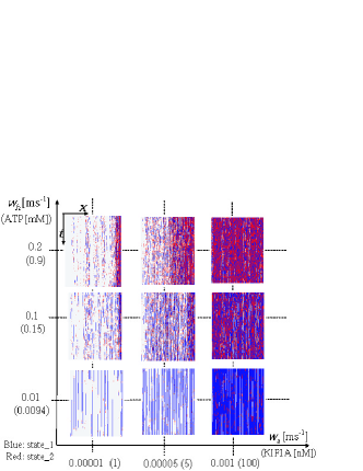
Figure 8: (Color online) Space-time plot of the model system for $c=1$. Each row of squares represents the state of the system at one single instant of time whereas successive rows (in the upward direction) correspond to the state of the system with increasing time. The blue and red squares indicate kinesins in the states $1$ and $2$, respectively, while the white squares correspond to empty binding sites on the microtubule. Total number of binding sites is $600$, and the configurations of the system are displayed for the last $1200$ time steps of a simulation run up to a total of $2\times 10^{5}$ time steps, starting from an initial state where all the binding sites on the microtubule were empty. The other model parameters are $\omega_{a}=0.3$,$\omega_{d}=0.2$, $\omega_{h}=400$,$\omega_{f}=600$,$\omega_{s}=200$,$\omega_{b}=50$ for bulk, and $\alpha=50$,$\beta_{1}=\beta_{2}=700$,$\gamma_{1}=\gamma_{2}=\delta=0$ for boundaries.

VI.1 Analytical treatment in the continuum limit

Let us first introduce the variable $x=\frac{i-1}{L-1}$; since $1\leq i\leq L$, we have $0\leq x\leq 1$. We map our system $(S_{i},W_{i})$ into $(S(x),W(x))$, and consider the continuum limit by considering $L$ to be large enough:

$$S(x\pm\epsilon)=S(x)\pm\epsilon\frac{\partial S}{\partial x}+\frac{\epsilon^{2}}{2}\frac{\partial^{2}S}{\partial x^{2}}$$ (50)

for $S(x\pm\epsilon)$ and a similar expansion for $W(x\pm\epsilon)$, where $\epsilon=1/L$. Using this Taylor expansion, we get

$$\frac{\partial S(x,t)}{\partial t} = \omega_{a}(1-S-W)+\omega_{s}W-(\omega_{h}+\omega_{d})S$$

$$+ \omega_{f}[W-\epsilon\frac{\partial W(x,t)}{\partial x}](1-S-W)$$

$$+ (1-c)\omega_{f}W(S+W$$

$$+\epsilon\frac{\partial S(x,t)}{\partial x}+\epsilon\frac{\partial W(x,t)}{\partial x})\,,$$

$$\frac{\partial W(x,t)}{\partial t} = c\omega_{f}W\left[S+W+\frac{\partial S(x,t)}{\partial x}\epsilon+\frac{\partial W(x,t)}{\partial x}\epsilon\right]$$ (51)

$$- (\omega_{s}+\omega_{f})W+\omega_{h}S\,.\$$

In the stationary state, we have

$$\epsilon\frac{\partial S(x)}{\partial x} = \frac{\omega_{s}+\omega_{f}}{c\,\omega_{f}}-\frac{\omega_{h}}{c\,\omega_{f}}\frac{S}{W}-(S+W)-\frac{\partial W(x)}{\partial x}\epsilon\,,$$

$$\epsilon\frac{\partial W(x)}{\partial x} = \frac{1}{1-S-W}(\frac{\omega_{a}}{\omega_{f}}+\frac{\omega_{s}+\omega_{f}-c\,\omega_{a}}{c\,\omega_{f}}W$$ (52)

$$- \frac{\omega_{h}+c(\omega_{a}+\omega_{d})}{c\,\omega_{f}}S-W(S+W).$$

Moreover, from the left boundary equations, by letting $S_{1}=S_{2}=S(0)$ and $W_{1}=W_{2}=W(0)$, we obtain

$$\alpha[1-S(0)-W(0)]-\omega_{h}S(0)+\omega_{s}W(0)$$

$$\hskip 28.45274pt+(1-c)\omega_{f}W(0)[S(0)+W(0)]=0$$ (53)

$$-(\omega_{s}+\omega_{f})W(0)+\omega_{h}S(0)$$

$$\hskip 56.9055pt+c\omega_{f}W(0)(S(0)+W(0))=0,$$ (54)

and, hence,

$$S(0) = \frac{\alpha-[c\,\alpha(\alpha-\omega_{s})/\omega_{f}]}{c\,\alpha+\omega_{h}}\,,$$

$$W(0) = \frac{\alpha}{\omega_{f}}\,.$$ (55)

Similarly from the right boundary conditions

$$-\omega_{h}S(1)+\omega_{s}W(1)-\beta S(1)$$

$$\hskip 28.45274pt+\omega_{f}W(1)[1-S(1)-W(1)]=0,$$ (56)

$$-\omega_{s}W(1)+\omega_{h}S(1)-\beta W(1)=0.$$ (57)

Solving these equations we have

$$S(1) = \frac{\omega_{s}+\beta}{\omega_{h}}\biggl{[}\frac{\omega_{h}}{\omega_{h}+\omega_{s}+\beta}-\frac{\beta}{\omega_{f}}\biggr{]}\,,$$

$$W(1) = \frac{\omega_{h}}{\omega_{h}+\omega_{s}+\beta}-\frac{\beta}{\omega_{f}}\,.$$ (58)

Note that the pair of coupled equations (52) involves only the first order derivatives of $S$ and $W$ with respect to $x$ whereas we have two sets of boundary conditions (55) and (58). Therefore, if we integrate the equations (52) using the boundary conditions (55), the solution may not, in general, match smoothly with the other solution obtained for the same equation using the boundary conditions (58). The discontinuity corresponds to a shock or domain wall.

The continuity condition gives $J_{l}=J_{r}$ where the flow just at the left side is denoted by $J_{l}=\omega_{f}h_{l}(1-r_{l}-h_{l})$ and that at the right is $J_{r}$. Thus we integrate (52) numerically by using (55) to the right end, and we also integrate them by (58) to the left end, and seek the point where $J_{l}=J_{r}$ is attained.

We have investigated the shock position by changing the values of $\omega_{a}$ and $\omega_{h}$. The results are given in Table 2 in the case $c=1$, which quantitatively agree with numerical simulations as shown in Fig. 9.

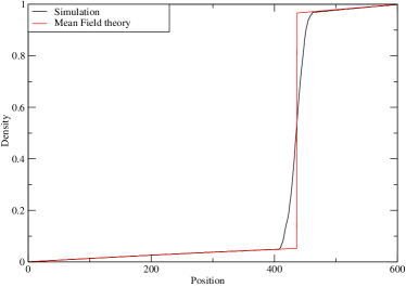
Figure 9: (Color online) An example of a density profile with shock obtained by integrating the mean-field equations as well as that of numerical result. Parameters are $\omega_{h}=200,\omega_{a}=0.01$.

$\omega_{h}$	$\omega_{a}$=0.01	$\omega_{a}$=0.025	$\omega_{a}$=0.05	$\omega_{a}$=0.065
200	0.725	0.5	0.318	0.253
150	0.776	0.571	0.382	0.311
125	0.808	0.618	0.425	0.35

Table 2: The position of the localized shock. Parameters are $L=600$, $c=1$, $\omega_{d}=\beta=0.1$, $\alpha=\omega_{a}$, $\omega_{f}=145$ and $\omega_{s}=55$.

VI.2 Shock position from simulations

In this subsection we locate the position of the shock in our model using a new shock tracking probe (STP) which is an extension of “second class particles” (SCP) janleb used earlier for locating domain walls in computer simulations of driven-diffusive lattice gas models defined on a discrete lattice. In the standard TASEP model, a SCP is defined as one that behaves as a particle while exchanging position with a hole and behaves as a hole while exchanging position with a particle. As a result, the second class particle has a tendency to get localized at the domain wall (or, the shock). Other types of STP have also been considered in the literature sakuntala

The rules for the movements of the STP in our model of KIF1A traffic have been prescribed by extending those for SCP in TASEP. Let us use the symbols $\bar{1}$ and $\bar{2}$ to denote the STPs which correspond to the states 1 and 2, respectively, of the particles. Now, in the special case $c=1$, we define the following rules for the movements of the STPs:

$$\begin{array}[]{ll}\bar{1}\to\bar{2}&\mbox{with rate }\omega_{h}\\ \bar{2}\to\bar{1}&\mbox{with rate }\omega_{s}\\ \bar{2}0\to 0\bar{1}&\mbox{with rate }\omega_{f}\\ \bar{2}0\to 0\bar{2}&\mbox{with rate }\omega_{b}\\ 0\bar{2}\to\bar{2}0&\mbox{with rate }\omega_{b}\\ 0X\cdots X\bar{X}\to\bar{X}X\cdots XX&\mbox{with rate }\omega_{a}\\ 2\bar{X}\to\bar{X}1&\mbox{with rate }\omega_{f}\\ 2\bar{X}\to\bar{X}2&\mbox{with rate }\omega_{b}\\ \bar{X}2\to 2\bar{X}&\mbox{with rate }\omega_{b}\end{array}$$ (59)

with $X$ and $\bar{X}$ denoting occupation in either state of particles or STPs respectively, while $\cdots$ denotes a line of sites occupied by particles. Further extension of these rules for arbitrary $c$ is straightforward.

These rules satisfy the STP-principle: if the selected site is a STP it behaves like a particle, while if the selected site is a particle it treats STPs in its vicinity as holes (by changing sites respectively). Note that there is no attachment and detachment of STPs. This is no problem after all, because $\omega_{a}$ and $\omega_{d}$ scale like $\frac{1}{L}$ with system size $L$ and we are only looking at a local quantity (the shock position), so they can be neglected for large systems (which we are interested in). Besides, for real (finite) systems they are negligibly small compared to the other rates $\omega_{h},\omega_{s},\omega_{f}$ and $\omega_{b}$. On the other hand, if the STPs were allowed to detach, the undesirable possibility of losing all the STPs through detachments could not be ruled out. Moreover, allowing STPs to attach and detach like the real particles would involve further subtleties of normalization during computation of averaged quantities.

A STP, which is not located at the shock, has a tendency to move to the shock position. Moreover, if a STP is already located at the shock, it follows the shock as the shock moves. For the purpose of illustration, consider first an idealized shock of the form …0000XXXXXX… Inserting a STP in either the low density region or the high density region it is obvious from the rules given in (59) that it will, on the average, move in the direction of the shock. However, in our model, the observed shocks are not ideal. Instead a few particles (holes) will appear in the low (high) density region. As a first approximation, one can assume that these particles (holes) are isolated, e.g. configurations like …00X000XXX0XX… Again, by careful use of the rules (59), one can show that the preferred motion of the STP is towards the location of the shock also in such realistic situations. This argument can be refined even further. In appendix B we present an analytical argument in mean-field approximation which supports the heuristic arguments used in the illustrative examples in this paragraph.

In addition to the rules listed above we define the following fusion rules:

$$\begin{array}[]{ll}\bar{2}\bar{X}\to 0\bar{1}&\mbox{with }\omega_{f}\\ \bar{2}\bar{X}\to 0\bar{2}&\mbox{with }\omega_{b}\\ \bar{X}\bar{2}\to\bar{2}0&\mbox{with }\omega_{b}\end{array}$$ (60)

The fusion rules ensure that if a shock exists, there will be a single STP in the system after sufficiently long time. This rule is extremely convenient because the lone STP will uniquely define the position of the sharp shock rather than a wide region of contiguous STPs separating the high-density and low-density regions.

For the practical implementation of the STPs on the computer, one has to select the initial positions of the STPs. We chose to put one STP at each end of the system at the beginning of the simulation. If a shock can exist in the system, the STPs move to the shock position, fuse and, finally, indicate the shock position. We determined the shock position in the stationary state by averaging over the fluctuating positions of the lone STP in the steady state. In contrast, survival of two STPs in the steady state of the system indicates absence of any shock; instead, these two STPs indicate the formation of boundary layers. Although the latter phenomenon could be interesting, we shall not discuss it here. We have compared the shock position obtained following the STP approach with that inferred from the density profiles measured by computer simulations of our model. These comparisons established that the rules (59) and (60), indeed, yield the correct results.

We determined numerically the mean position of shock in a system with $L=600$ sites as a function of $\omega_{a}$ and $\omega_{h}$ which is shown as a 3D-plot in Fig. 10.

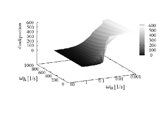
Figure 10: Shock position as function of $\omega_{a}$ and $\omega_{h}$ obtained from STP simulations.

In Fig. 11 we have plotted the shock positions as a function of the parameter $c$ for different choices of $\omega_{s}$ and $\omega_{f}$. In this figure, one observes two plateaus connected by a decaying domain (leftshift of the shock position). It seems that upper plateau approximately ends for $c=1-\omega_{s}-\omega_{f}$. Further detailed investigations will be needed to decide whether the sharp change in the position of the shock at this value of $c$ indicates merely a crossover or a signature of a genuine phase transition.

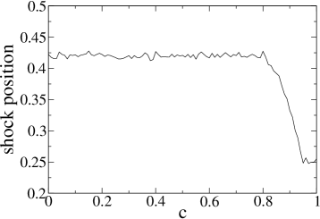
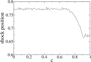
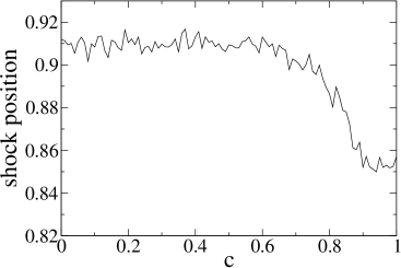
Figure 11: Variation of the shock positions with the interaction parameter $c$ for system size $L=3000$, $\omega_{d}=0.1$ and: top: $\omega_{s}=55,\,\omega_{f}=145$, $\omega_{a}=0.007$, $\omega_{h}=180$; middle: $\omega_{s}=100,\,\omega_{f}=200$, $\omega_{a}=0.1$, $\omega_{h}=300$; bottom: $\omega_{s}=100,\,\omega_{f}=300$, $\omega_{a}=0.01$, $\omega_{h}=130$

VII Analytical Phase diagram without Langmuir dynamics

In this section we derive the phase diagram in the plane spanned by the boundary rates $\alpha$ and $\beta$ for the special case of our model where attachments and detachment of the motors do not take place. In other words, we derive the phase diagram of our model in the $\alpha-\beta$-plane in the absence of Langmuir kinetics. We use the domain wall theory proposed in kolo to derive this phase diagram from the flow-density relation (31) of the corresponding periodic system. From this study, one can calculate the collective velocity and the shock velocity which determine the dynamics of the density profiles of the open system. Note that, because of the translational invariance of the periodic system, $S$ and $W$ show constant density profiles.

The collective velocity $v_{c}$ of this system is given by

$$v_{c} = \frac{\partial J(\rho)}{\partial\rho}$$

$$= \omega_{f}\omega_{h}\frac{c\omega_{f}\rho^{2}-2(\omega_{h}+\omega_{s}+\omega_{f})\rho+\omega_{h}+\omega_{s}+\omega_{f}}{(\omega_{h}+\omega_{s}+\omega_{f}(1-c\rho))^{2}}.$$

Thus $v_{c}=0$ gives the critical density

$$\rho_{c}=k-\sqrt{k(k-1)}$$ (62)

where

$$k=\frac{\omega_{h}+\omega_{s}+\omega_{f}}{c\omega_{f}}$$ (63)

for the case $c\neq 0$, and $\rho_{c}=1/2$ for the case $c=0$. Note that $k$ is always larger than 1. Next we calculate the shock velocity

$$S=\frac{J(\rho_{L})-J(\rho_{R})}{\rho_{L}-\rho_{R}},$$ (64)

where we take $\rho_{L}=\alpha$ and $\rho_{R}=1-\beta$. Then we have

$$S=(\omega_{h}+\omega_{s}+\omega_{f})(\beta-\alpha)+c\omega_{f}\alpha(1-\beta).$$ (65)

From $S=0$ we obtain the first order phase transition curve

$$\beta=(1-k)\left(1+\frac{k}{\alpha-k}\right),$$ (66)

that starts at $\alpha=0$ and ends at $\alpha=\rho_{c}$ (Fig. 12). This curve separates the low and high density phase.

Figure 12: Phase diagram of this system without Langmuir dynamics.

VIII Experimental investigation with KIF1A

In the experiments performed by Okada nosc , microtubules labeled with a green fluorescent dye were immobilized on the top surface of the cell. The single-headed kinesins labeled with a red fluorescent dye were then introduced into the cell together with with ATP. The movement of the motor proteins was observed using imaging techniques of optical microscopy described in okada1 . A “comet-like” structure, as shown in Fig. 13, was formed by the kinesins (red) on the microtubule (green). The first two images from the top, which correspond to low and moderate densities, respectively, were taken under essentially same conditions, but the lowermost image in the figure was taken with smaller intensifier gain, because it is too bright for the intensifier.

No special filtering was applied to the original image. Each red fluorescent spot in Fig. 13 normally corresponds to a single fluorescently-labeled kinesin molecule, if the density is not too high (top panel of Fig. 13 is a typical example of such cases). Due to the optical resolution limit (about 500 nm), more than one kinesin can together form a single brighter spot when the motors are too close to be resolved (as happens, for example, in the middle panel of Fig. 13). Nevertheless, even in such situations, the number of fluorochromes in each spot can be estimated from its intensity. At much higher densities (for example, that corresponding to the bottom panel of Fig. 13), fluorescent signals are no longer separable as spots. Even in such cases, the density of fluorochromes can be estimated from their intensity profile. However, Okada measured the intensity profile just to confirm that each spot corresponds to a single kinesin molecule in the lowest density experiment. In other words, at low densities, the density of the fluorescent spots gives a good estimate for the density of kinesins. But, at higher densities, the spot density gives an underestimate of the kinesin density due to the overlap of fluorescent spots (which are not visually separable because of the limited resolution).

It is true that, under normal physiological conditions, the global density of motors in a cell never oversaturates the microtubule surface as happened in Okada’s experiment described above. However, so far as the in-vivo situations are concerned, the motors and microtubules are heterogeneously distributed in cells. Thus, the local density of motors and microtubule surfaces might be a direct determinant of the formation of motor traffic jam within cells during in-vivo experiments. Moreover, in pathological situations, traffic jam on microtubule-based transport systems, such as axonal transport, is not rare. In fact, such traffic jams have been implicated in many neurodegenerative diseases goldd1 ; goldd2 ; mandeld1 . Many putative factors may contribute to the “jammorigenesis”; these include the population of the active motor proteins, the presence of the inactive motor proteins, the number of “obstacles” on the microtubule surface such as microtubule associated proteins, and so on. Obviously, these factors should be, ultimately, incorporated into a more “realistic” extended version of our model in order to explicitly account for the observed “jammorigenesis”. The current version of our model is just the minimal one.

These experimental results have three important implications. First, traffic jam can actually take place in living cells at least in some experimental conditions. Second, the local concentration, rather than the global concentration, of the motors determines whether or not jam will form in a living cell. Even in the overexpressing cells, the overall concentration of motors is much lower than that of tubulin. But still “comet” is formed. Third, negative regulation systems, which are not included in the current version of our model, prevent jam formation in physiological situations.

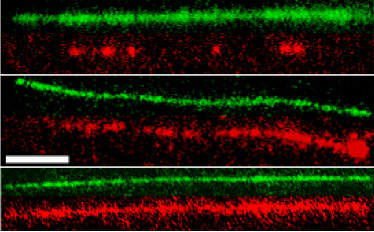
Figure 13: (Color online) A “comet-like” structure formed by kinesins (red) on the microtubule (green). The high-density and low-density regions are clearly separated in this image. The white bar length is 2 $\mu$m.

IX Discussion

In this paper we have proposed a biologically motivated extension of our recent quantitative model nosc describing traffic-like collective movement of single-headed kinesin motors KIF1A. The dynamics of the system has been formulated in terms of a stochastic process where position of a motor is repesented by a discrete variable and time is continuous. The model explicitly captures the most essential features of the biochemical cycle of each motor by assigning two discrete internal (“chemical” or “conformational”) states to each motor. The model not only takes into account the exclusion interactions, as in the previous models, but also includes a possible interaction of motors that controls ADP release rates by introducing a free parameter $c$. To our knowledge okadapc , it is not possible even to establish the existence of this mechano-chemical interaction with the experimental data currently available in the literature. However, we hope that our results reported here will help in developing experimental methods which will not only test the existence of this interaction but also its strength if it exists. For example, we have predicted the dependence of the shock position on $c$ (and, therefore, that of $c$ on the shock position). Thus, at least in prinicple, one could determine $c$ by comparing the experimentally measured shock position with this relation. The $c$-dependence of some of the other quantities reported here may provide alternative, and possibly, more direct way of estimating the strength of this mechano-chemical interaction.

We have compared and contrasted our model and the results with earlier generic models of single motors as well as those of motor traffic. Our analytical treatment of the dynamical equations in the continuum limit (i.e., a limit in which the spatial position of each motor is denoted by a continuous variable) has also established the occurrence of a non-propagating shock in this model. We have also calculated the position of this shock numerically using the method of second class particles.

Mean field treatment of the rate equations for $c=0$ showed that this special case of our model is equivalent to the simpler PFF model which also predicts two-phase coexistence (where the two phases are separated by a non-propagating shock). One can argue analytically pgdiplom ; popkov , as we also observed in simulations, that the general features of the $\alpha-\beta$-phase diagrams of our model is the same as those for the PFF model. Thus, the PFF model, in spite of its simplicity, captures the essential generic features of intracellular transport. But, it is not possible to make direct quantitative comparison between the predictions of the PFF model and experimental data as the parameters of the PFF model are not accessible to direct biochemical experiments. In contrast, our model captures the essential features of the internal biochemical transitions of each single-headed kinesin and we could establish a one to one correspondence between our model parameters and measurable quantities. The concentrations of the kinesin motors and ATP are two such important parameters both of which which are variable in-vivo and can be controlled in in-vitro-experiments. We have reported the phase diagram of our model in the plane spanned by these experimentally accessible parameters.

Finally, we have summarized evidences for the formation of molecular motor jam from Okada’s in-vitro experiments nosc and discussed their relevance in intra-cellular transport under physiological conditions.

Appendix A: A GENERALIZED MODEL OF NON-INTERACTING MOTORS

In order to make a comparison between the non-interacting limit of our model and the earlier models of non-interacting molecular motors, we consider here a slightly more general model which allows “reverse” transitions for each of the “forward” transitions. Then we show that the non-interacting limit of our model is a special case of the general model while some other special cases correspond to earlier models of non-interacting motors.

Figure 14: Schematic description of a general three-state model of a single molecular motor.

Consider the multi-step chemical kinetic scheme shown in the Fig. 14. Note that this generalized scheme garaithesis allows a transition from the strongly bound state at $i+1$ to the weakly bound state at $i$ with the rate constant $\omega_{f}^{-}$ which is not allowed in our model shown in fig.2. In fact, in this generalized scheme, corresponding to every forward step (those corresponding to $\omega_{f}^{+}$, $\omega_{h}^{+}$ and $\omega_{b}$) there is a backward step (corresponding to $\omega_{f}^{-}$, $\omega_{h}^{-}$ and $\omega_{b}$, respectively). This generalization is in the spirit of Fisher-Kolomeisky-type multi-step chemical kinetic models of molecular motors kolo1 ; kolo2 ; kolo3 where each of the reactions are allowed to be reversible, albeit with different rate constants, in general.

In the mean-field limit the the master equations governing the dynamics of this general model in the bulk are given by

$$\frac{dS_{i}}{dt} = \omega_{a}(1-S_{i}-W_{i})+\omega_{f}^{+}W_{i-1}$$ (67)

$$+ \omega_{h}^{-}W_{i}-\omega_{h}^{+}S_{i}-\omega_{f}^{-}S_{i}-\omega_{d}S_{i},$$

$$\frac{dW_{i}}{dt} = \omega_{h}^{+}S_{i}+\omega_{f}^{-}S_{i+1}-\omega_{h}^{-}W_{i}-\omega_{f}^{+}W_{i}$$ (68)

$$+ \omega_{b}(W_{i-1}+W_{i+1})-2\omega_{b}W_{i}.$$

Imposing periodic boundary conditions, the steady state solutions for $S$ and $W$ can be written as

$$S=\frac{\omega_{a}(\omega_{h}^{-}+\omega_{f}^{+})}{\omega_{a}(\omega_{h}^{-}+\omega_{f}^{+}+\omega_{h}^{+}+\omega_{f}^{-})+\omega_{d}(\omega_{h}^{-}+\omega_{f}^{+})},$$ (69)

$$W=\frac{\omega_{a}(\omega_{h}^{+}+\omega_{f}^{-})}{\omega_{a}(\omega_{h}^{-}+\omega_{f}^{+}+\omega_{h}^{+}+\omega_{f}^{-})+\omega_{d}(\omega_{h}^{-}+\omega_{f}^{+})}\,.$$ (70)

Hence,

$$S+W=\frac{\omega_{a}(\omega_{h}^{-}+\omega_{f}^{+}+\omega_{h}^{+}+\omega_{f}^{-})}{\omega_{a}(\omega_{h}^{-}+\omega_{f}^{+}+\omega_{h}^{+}+\omega_{f}^{-})+\omega_{d}(\omega_{h}^{-}+\omega_{f}^{+})}.\,$$ (71)

The corresponding steady-state flux

$$J=W_{i}\omega_{f}^{+}-S_{i+1}\omega_{f}^{-}\,$$ (72)

is given by

$$J=\frac{\omega_{f}^{+}\omega_{h}^{+}-\omega_{f}^{-}\omega_{h}^{-}}{(K+1)(\omega_{h}^{-}+\omega_{f}^{+})+(\omega_{h}^{+}+\omega_{f}^{-})}.$$ (73)

The relation between this generalized model of non-interacting motors and the non-interacting limit of our model is quite straightforward. In the special case $\omega_{f}^{-}=0$, using the identification $\omega_{f}^{+}=\omega_{f}$, $\omega_{h}^{+}=\omega_{h}$ and $\omega_{h}^{-}=\omega_{s}$, the equations (69), (70) and (73) reduce to the equations (22), (23) and (24), respectively.

Appendix B: A MF ARGUMENT FOR MOVEMENT OF STP AND SHOCK POSITION

In this appendix we argue that a STP will move to the location of the shock, if a shock exists in the system. Our arguments are based on an analysis in the mean-field approximation. The master equations for the probabilities of the STP, which correspond to the equations (14) for the real particles, are given by

$$\frac{d}{dt}S_{i}^{(2)} = \omega_{f}W_{i-1}^{(2)}(1-\rho_{i}^{(1)})+\omega_{f}W_{i}^{(1)}S_{i+1}^{(2)}-\omega_{f}W_{i-1}^{(1)}S_{i}^{(2)}$$ (74)

$$- \omega_{h}S_{i}^{(2)}+\omega_{s}W_{i}^{(2)}+\omega_{f}(1-c)W_{i}^{(2)}\rho_{i+1}^{(1)},$$

$$\frac{d}{dt}W_{i}^{(2)} = \omega_{h}S_{i}^{(2)}-\omega_{s}W_{i}^{(2)}-\omega_{f}W_{i}^{(2)}(1-\rho_{i+1}^{(1)})$$ (75)

$$- \omega_{f}W_{i-1}^{(1)}W_{i}^{(2)}+\omega_{f}W_{i}^{(1)}W_{i+1}^{(2)}$$

$$-\omega_{f}(1-c)W_{i}^{(2)}\rho_{i+1}^{(1)},$$

where $S_{i}^{(2)}$ and $W_{i}^{(2)}$ represent the probabilities of finding the STP in the weakly ($W^{(2)}$) and strongly ($S^{(2)}$) bound states, respectively, at the site $i$; note that $S_{i}^{(1)}$ and $W_{i}^{(1)}$ are the corresponding probabilities for the real particles. Obviously, $\rho_{i}^{(1,2)}=S_{i}^{(1,2)}+W_{i}^{(1,2)}$.

Adding the two equations (74) and (75) we obtain

$$\frac{d}{dt}\rho_{i}^{(2)} = (\omega_{f}W_{i-1}^{(2)}(1-\rho_{i}^{(1)})-\omega_{f}W_{i-1}^{(1)}\rho_{i}^{(2)})$$ (76)

$$- (\omega_{f}W_{i}^{(2)}(1-\rho_{i+1}^{(1)})-\omega_{f}W_{i}^{(1)}\rho_{i+1}^{(2)}).$$

Comparing this with the equation of continuity $d\rho_{i}/dt=J_{i-1}-J_{i}$, we identify the current $J_{i}^{STP}$ of STP on site $i$ to be

$$J_{i}^{STP}=\omega_{f}W_{i}^{(2)}(1-\rho_{i+1}^{(1)})-\omega_{f}W_{i}^{(1)}\rho_{i+1}^{(2)}.$$ (77)

Consider a situation where we have one STP in a continuous region of particles (with no shock inside), so we can put $\rho_{i}^{(1)}\approx\rho_{i+1}^{(1)}=:\rho^{(1)};\,S_{i}^{(1)}\approx S_{i+1}^{(1)}=:S^{(1)}$ and $W_{i}^{(1)}\approx W_{i+1}^{(1)}=:W^{(1)}$. We assume that, after sufficiently long time, the internal states of the STP relax to a stationary state so that the probabilities of finding the STP in the strongly-bound and weakly-bound states are independent of time. However, the mean position of the STP might still change with time.

Then, ${\cal{S}}:=\sum_{i}S_{i}^{(2)}$ is the probability of finding the STP in a strongly bound state, while the corresponding probability of finding the STP in the weakly bound state is ${\cal{W}}:=\sum_{i}W_{i}^{(2)}$ where the summations are over an interval of length $l$ that contains no shocks and one single STP. Obviously, ${\cal{S}}+{\cal{W}}=1$. Using (75) we have

$$0=\frac{d}{dt}{\cal W} = \omega_{h}{\cal S}-\omega_{s}{\cal W}-\omega_{f}{\cal W}+\omega_{f}\rho^{(1)}{\cal W}$$ (78)

$$- \omega_{f}(1-c)\rho^{(1)}{\cal W},$$

where we have used the fact that

$$\omega_{f} \sum_{i}W_{i}^{(1)}W_{i+1}^{(2)}-W_{i-1}^{(1)}W_{i}^{(2)}$$

$$= \omega_{f} W^{(1)}(\sum_{i}W_{i+1}-\sum_{i}W_{i-1})=0.$$ (79)

Solving equation (78) for ${\cal W}$, we obtain

$${\cal W}=\frac{\omega_{h}}{\omega_{h}+\omega_{s}+(1-c\rho^{(1)})\omega_{f}}.$$ (80)

The results derived above are valid for any density distribution of STPs as long as there is a shock-free neighbourhood of the STP and the particles are in a steady state. Now consider a specific configuration where a STP is given to be located at the site $i$ while its internal state remains unspecified. In this case,

$$\rho_{k}^{(2)}=\delta_{ik}.$$ (81)

Then we have ${\cal{W}}=W_{i}^{(2)}$ for any summation interval that includes the site $i$. Of course, $W_{k}^{(2)}=0$ for $k\neq i$ for this distribution of $\rho_{k}$. Therefore, using (80) we obtain

$$W_{k}^{(2)}=\frac{\omega_{h}\delta_{ik}}{\omega_{h}+\omega_{s}+(1-c\rho^{(1)})\omega_{f}}.$$ (82)

The analogous solution for $W^{(1)}$ obtained from (32) is

$$W^{(1)}=\frac{\omega_{h}\rho^{(1)}}{\omega_{h}+\omega_{s}+(1-c\rho^{(1)})\omega_{f}}.$$ (83)

For the density distribution considered here, we can take the current as an effective hopping rate of the STP to the right, i.e., $q_{i}^{r}=J_{i}(\{\rho_{k}^{(2)}=\delta_{ik}\})$. Similarly, we have effective hopping rate of the STP to the left $q_{i}^{l}=-J_{i-1}(\{\rho_{k}^{(2)}=\delta_{ik}\})$. Inserting (83) and (82) into (77) for $\rho_{k}^{(2)}=\delta_{ik}$, we obtain

$$q_{i}^{r}-q_{i}^{l}=\frac{\omega_{f}\omega_{h}}{\omega_{h}+\omega_{s}+(1-c\rho^{(1)})\omega_{f}}(1-2\rho^{(1)}).$$ (84)

Note that the fraction in (84) is always positive. Therefore, if a STP is in a low density region with $\rho^{(1)}<\frac{1}{2}$, we have $q_{i}^{r}-q_{i}^{l}>0$ and the STP tends to hop to the right. But, if the STP is in a high density region with $\rho^{(1)}>\frac{1}{2}$, we have $q_{i}^{r}-q_{i}^{l}<0$ and its prefered direction of hopping is left. Thus, in the continuum limit, if there is one shock separating a low density region at the left and a high density region at the right, any single STP will be driven to this domain wall. For sufficiently long time the average position of the STP will be equal to the shock position.

References

- (1) M. Schliwa, (ed.) Molecular Motors, (Wiley-VCH, 2003).
- (2) J. E. Molloy and C. Veigel (eds.), Special issue of IEE Proceedings-Nanobiotechnology, 150, No.3 (December, 2003).
- (3) Special issue of J. Phys. Cond. Matt. 17, no.47 (2005).
- (4) D. Chowdhury, A. Schadschneider and K. Nishinari, Phys. of Life Rev. 2, 318 (2005).
- (5) J. Howard, Mechanics of motor proteins and the cytoskeleton, (Sinauer Associates, 2001).
- (6) C. Bustamante, D. Keller and G. Oster, Acc. Chem. Res. 34, 412-420 (2001).
- (7) M. Aridor and L.A. Hannan, Traffic 1, 836-851 (2000); 3, 781-790 (2002).
- (8) C. MacDonald, J. Gibbs and A. Pipkin, Biopolymers, 6, 1 (1968).
- (9) B. Schmittmann and R.K.P. Zia, in: Phase Transition and Critical Phenomena, Vol. 17, eds. C. Domb and J. L. Lebowitz (Academic Press, 1995).
- (10) B. Derrida, Phys. Rep. 301, 65 (1998)
- (11) G. M. Schütz, Phase Transitions and Critical Phenomena, vol. 19 (Acad. Press, 2001).
- (12) R. Lipowsky, S. Klumpp, and T. M. Nieuwenhuizen, Phys. Rev. Lett. 87, 108101 (2001).
- (13) A. Parmeggiani, T. Franosch and E. Frey, Phys. Rev. Lett. 90, 086601 (2003).
- (14) M.R. Evans, R. Juhasz and L. Santen, Phys. Rev. E 68, 026117 (2003).
- (15) V. Popkov, A. Rakos, R.D. Williams, A.B. Kolomeisky and G.M. Schütz, Phys. Rev. E 67, 066117 (2003).
- (16) A. Parmeggiani, T. Franosch and E. Frey, Phys. Rev. E 70, 046101 (2004).
- (17) R. Lipowsky, Y. Chai, S. Klumpp, S. Liepelt and M. J.I. Müller, Physica A 372, 34 (2006) and references therein.
- (18) K. Nishinari, Y. Okada, A. Schadschneider and D. Chowdhury, Phys. Rev. Lett. 95, 118101 (2005)
- (19) Y. Okada and N. Hirokawa, Science 283, 1152-1157 (1999).
- (20) Y. Okada and N. Hirokawa, Proc. Natl. Acad.Sciences USA 97, 640-645 (2000).
- (21) M. Kikkawa, E.P. Sablin, Y. Okada, H. Yajima, R.J. Fletterick and N. Hirokawa, Nature 411, 439-445 (2001).
- (22) Y. Okada, H. Higuchi and N. Hirokawa, Nature, 424, 574-577 (2003).
- (23) R. Nitta, M. Kikkawa, Y. Okada and N. Hirokawa, Science 305, 678-683 (2004).
- (24) K. Sasaki, J. Phys. Soc. Jap. 72, 2497-2508 (2003)
- (25) F. Jülicher, A. Ajdari and J. Prost, Rev. Mod. Phys. 69, 1269-1281 (1997).
- (26) P. Reimann, Phys. Rep. 361, 57-265 (2002).
- (27) Y. Okada, Private communication.
- (28) Yi-der Chen, Biophys. J. 78, 313 (2000).
- (29) M. E. Fisher and A. B. Kolomeisky, Proc. Nat. Acad. Sci. 96, 6597 (1999); Physica A 274, 241 (1999).
- (30) A. B. Kolomeisky and M.E. Fisher, Physica A 279, 1 (2000).
- (31) A. B. Kolomeisky, J. Chem. Phys. 115, 7253 (2001).
- (32) A. B. Kolomeisky, G. Schütz, E. B. Kolomeisky and J. P. Straley, J. Phys. A 31, 6911 (1998); V. Popkov and G. M. Schütz, Europhys. Lett. 48, 257 (1999).
- (33) Philip Greulich, Diploma Thesis, Cologne University (2006)
- (34) S.A. Janowsky, J.L. Lebowitz, Phys. Rev. A45, 618 (1992)
- (35) S. Chatterjee and M. Barma, cond-mat/0611675 (2006).
- (36) L.S. Goldstein, Proc. Natl. Acad. Sci. 98, 6999-7003 (2001).
- (37) L.S. Goldstein, Neuron 40, 415-425 (2003).
- (38) E. Mandelkow and E.M. Mandelkow, Trends in Cell Biol. 12, 585-591 (2002).
- (39) A. Garai, Thesis (in preparation).