Dose distribution in water for monoenergetic photon point sources in the energy range of interest in brachytherapy: Monte Carlo simulations with PENELOPE and GEANT4

Abstract

Monte Carlo calculations using the codes PENELOPE and GEANT4 have been performed to characterize the dosimetric properties of monoenergetic photon point sources in water. The dose rate in water has been calculated for energies of interest in brachytherapy, ranging between 10 keV and 2 MeV. A comparison of the results obtained using the two codes with the available data calculated with other Monte Carlo codes is carried out. A $\chi^{2}$-like statistical test is proposed for these comparisons. PENELOPE and GEANT4 show a reasonable agreement for all energies analyzed and distances to the source larger than 1 cm. Significant differences are found at distances from the source up to 1 cm. A similar situation occurs between PENELOPE and EGS4.

I Introduction

Dosimetry of monoenergetic point sources is interesting from different points of view. Dose distributions around more complex sources (e.g. polyenergetic sources or sources with finite dimensions) can be calculated using the monochromatic source data, providing the corresponding modifications to account for the source geometry and the capsule materials are made.

Dose distributions generated by monoenergetic point sources constitute a crucial test to compare Monte Carlo (MC) radiation transport codes, because the differences observed in the simulation results can be linked to the basic physics taken into account by these codes.

In case of photons, the most complete available databases of dose distributions in water for monoenergetic point sources are those of Berger (1968) and Luxton and Jozsef (1999). Berger solved the one-dimensional Boltzmann transport equation and showed results for energies ranging between 15 keV and 3 MeV. He provided polynomial expansions of the energy-absorption buildup factors needed to calculate the corresponding dose rates.

More recently, Luxton and Jozsef (1999) have used the EGS4 MC code to determine these dose distributions for 10 keV to 2 MeV photons. These authors have found a good agreement with Berger’s results (within 1%) between 40 and 400 keV. Some discrepancies have been quoted for energies below 40 keV, where differences reach 4-5%. Above 500 keV, Luxton and Jozsef have found a buildup in the radial dose distribution not shown in the results of Berger. Between 1 and 2 MeV, discrepancies are $\sim$4%. Finally, EGS4 results suggest an additional structure at $\sim$3 cm from the 2 MeV source, which the authors have guessed to be an artifact of the MC simulation.

The MC code PENELOPE (v. 2001) (Salvat et al., 2001) has been benchmarked for low-energy photons (10-150 keV) by Ye et al. (2004). These authors have compared the doses calculated with PENELOPE and MCNP4C to the results of Luxton and Jozsef (1999) obtained with EGS4. They paid special attention to the differences due to the various libraries used: EPDL97 (Cullen et al., 1997) for PENELOPE, DLC-200 (Frankle and Little, 2000) and the updated DLC-146 for MCNP4C and PHOTX (Sakamoto, 1993) for EGS4. Ye et al. found that all the results agreed rather well except those obtained with MCNP4C and the DLC200 library below 100 keV for which the dose rates are up to 9% lower than for the other cases.

In their MC simulations, Ye et al. (2004) used a cylindrical liquid water phantom with 30 cm diameter. For energies above 100 keV, Ye et al. observed discrepancies between their calculations and those of Luxton and Jozsef (1999) which they ascribed to the fact that these authors used an infinite water phantom.

In this work, new simulations of monoenergetic photon point sources in the range 10 keV to 2 MeV embedded in water are performed using the MC codes PENELOPE (Salvat et al., 2001, 2003) and GEANT4 (Agostinelli et al., 2003; GEANT4, 2006). Our purpose is to benchmark the PENELOPE and GEANT4 codes for this energy range by intercomparing our results with those found by Luxton and Jozsef (1999), with EGS4, and by Ye et al. (2004), also with PENELOPE but with a different scoring geometry.

II Material and Methods

II.1 Monte Carlo codes

In this work PENELOPE (v. 2001) (Salvat et al., 2001) and (v. 2003) (Salvat et al., 2003) and GEANT4 (Agostinelli et al., 2003; GEANT4, 2006) (v. 4.5.2) MC codes have been used to perform the simulations.

PENELOPE is a general purpose MC code which performs simulations of coupled electron-photon transport. It can be applied for energies ranging from a few hundred eV up to 1 GeV and for arbitrary materials. Besides, PENELOPE permits a good description of the particle transport at the interfaces and presents a more accurate description of the electron transport at low energies in comparison to other general purpose MC codes. These characteristics make PENELOPE to be an useful tool for medical physics applications as previous works have pointed out (see e.g. Sánchez-Reyes et al., 1998; Asenjo et al., 2002; Al-Dweri et al., 2004). Details about the physical processes considered can be found in Salvat et al. (2001, 2003).

GEANT4 is a toolkit for simulating the passage of particles through matter for applications in high energy physics, nuclear experiments, medical physics studies, etc. Due to its purpose, the available energy range and the possible particles to be simulated are much larger than in PENELOPE. GEANT4 includes low energy packages which permit to extend the validity range of particle interactions for electrons, positrons and photons down to 250 eV, and can be used up to approximately 100 GeV. A general description of the GEANT4 toolkit can be found in Agostinelli et al. (2003). A detailed documentation concerning the physics involved can be found in GEANT4 (2006). In our calculations the low-energy package G4EMLOW.2.3 has been used.

II.2 Simulations

In the simulations performed we have used an infinite water phantom which we have labeled $\mathcal{P}_{\rm inf}$. In this case the scoring voxels have been chosen to be concentric spherical shells with thickness 0.5 mm and centered in the point source. The size of these scoring voxels avoids the possible volume averaging artifacts that could appear using larger voxels.

Besides, we have performed additional simulations with a spherical finite phantom with a radius of 15 cm, filled with water and with the point source situated at its center. We have labeled $\mathcal{P}_{\rm fin}$ this phantom and we have used the same scoring voxels as in $\mathcal{P}_{\rm inf}$.

As the sources studied are point sources, the different quantities simulated (e.g., the dose rate, $\dot{D}(r)$), depend on the distance between the target point and the source, $r$.

In our simulations, the energy deposited in each voxel $j$, $E^{j}$, was scored to obtain the histograms corresponding to $\dot{D}(r)$. We labeled $\dot{D}^{j}$ the value corresponding to the $j$-th voxel. In order to avoid the effect of the geometric factor ($r^{-2}$ in this case) which dominates $\dot{D}(r)$, we have calculated also the quantity

$$R(r)\,=\,r^{2}\,\dot{D}(r)\,.$$ (1)

We have simulated this quantity by scoring directly $(r^{2}E)$, thus obtaining $R^{j}$ for each scoring shell $j$. However, in common practice (see e.g. Luxton and Jozsef 1999), this quantity is calculated as

$$R^{j}_{\rm M}\,=\,(r^{j}_{\rm M})^{2}\,\dot{D}^{j}\,,$$ (2)

for each bin $j$ of the histogram corresponding to $\dot{D}(r)$. In this equation

$$r^{j}_{\rm M}\,=\,\frac{r^{j}_{>}+r^{j}_{<}}{2}\,,$$ (3)

with $r^{j}_{<}$ and $r^{j}_{>}$ the minimum and maximum $r$ values corresponding to the $j$-th “detector” voxel.

The results for $R(r)$ obtained with the phantoms $\mathcal{P}_{\rm inf}$ and $\mathcal{P}_{\rm fin}$ can be found in http://fm137.ugr.es/PhotonPointSources/ for both PENELOPE (v. 2003) and GEANT4. A total of 40 energies in the range between 10 keV and 2 MeV have been considered. In these tables, also the air kerma strengths and the dose rate constants calculated with PENELOPE and GEANT4 are given.

II.3 Simulation parameters

PENELOPE considers analog simulation for photons. Electrons and positrons are simulated by means of a mixed scheme in which collisions are classified as “hard” and “soft”. Hard collisions are characterized by a scattering angle or an energy loss larger than certain cutoff values and are individually simulated. A multiple scattering theory is used to describe the soft collisions, in which the polar angular deflection and the energy loss are below the threshold values. The electron tracking is controlled by means of four parameters. $C_{1}$ and $C_{2}$ refer to elastic collisions. $C_{1}$ gives the average angular deflection due to a elastic hard collision and to the soft collisions previous to it. $C_{2}$ represents the maximum value permitted for the average fractional energy loss in a step. On the other hand, $W_{\rm cc}$ and $W_{\rm cr}$ are energy cutoffs to distinguish hard and soft events. Thus, the inelastic electron collisions with energy loss $W<W_{\rm cc}$ and the emission of bremsstrahlung photons with energy $W<W_{\rm cr}$ are considered in the simulation as soft interactions. In addition the maximum step size can be controlled using the parameter $s_{\rm max}$.

In our simulations with PENELOPE, the parameters were fixed to the following values: $W_{\rm cc}=10$ keV, $W_{\rm cr}=1$ keV, $C_{1}=C_{2}=0.05$. Photons were simulated down to 1 keV. Electrons and positrons were absorbed when they slow down to kinetic energies of 10 keV. We have checked that the use of lower values for these parameters does not cause changes in the results. Finally, $s_{\rm max}$ was taken to be $10^{35}$ cm.

In case of GEANT4 simulations, it is necessary to choose a range threshold for each particle type. This threshold is converted, internally, to an energy threshold below which secondary particles are not emitted. In our calculations the range thresholds have been fixed to values providing energy thresholds of 1 keV and 10 keV for photons and electrons, respectively. Besides, one can select for electrons the values of the maximum step size, the variable $dRoverRange$, which is the maximum fraction of the stopping range that an electron can travel in a step, the variable $finalRange$, which establishes the limit for the gradual reduction of the step size, and, finally, the variable $f_{r}$, which controls the step size when the electron is transported away from a boundary into a new volume. In our simulations we have used the default values for these parameters (no maximum step size, $dRoverRange=1$, $finalRange=1$ mm, and $f_{r}$=0.2). We have performed a series of calculations using $dRoverRange=0.01$ and $finalRange=100$ nm. These values were used by Poon et al. (2005) to investigate the consistency of GEANT4 in geometries including ionization chambers, which is a more exigent situation than ours concerning the electron transport. However, we have not found any difference between the results obtained with this new set of parameters and the previous one, in the energy range we have considered.

II.4 Statistics

In the simulations we scored the energy deposited by all the particles of the $i$-th history (that is, including the primary particle and all the secondaries it generates) in the $j$-th voxel. We label the value obtained $E^{j}_{i}$. This permits to obtain the MC estimate of the average value of $E^{j}$ (per initial particle), which is given by

$$\overline{E}^{j}\,=\,\frac{1}{N}\sum_{i=1}^{N}E^{j}_{i}\,.$$ (4)

Here $N$ is the number of simulated histories. In addition, $(E^{j}_{i})^{2}$ was also scored in order to calculate the statistical uncertainties which are given by

$$\sigma_{\overline{E}^{j}}\,=\,\sqrt{\frac{1}{N}\left[\frac{1}{N}\sum_{i=1}^{N}(E^{j}_{i})^{2}\,-\,(\overline{E}^{j})^{2}\right]}\,.$$ (5)

We have proceed in a similar way with $(r^{2}E)^{j}$. The uncertainties given below correspond to 1$\sigma$. Except when explicitly mentioned, all simulations have been performed following $3\cdot 10^{7}$ histories. This permitted us to maintain these statistical uncertainties under reasonable levels.

II.5 Comparison of histograms

The usual outputs of the MC simulations of radioactive sources include histograms corresponding to the magnitudes of interest. Then, the benchmark of the codes used is done by comparing either the histograms by-eye in a figure or a restricted set of values corresponding to different bins in a table.

To gain more insight, it is useful to plot the relative difference between the two histograms $H_{1}$ and $H_{2}$, which is given by

$$\Delta^{j}_{H_{1},H_{2}}\,=\,\displaystyle\frac{H_{1}^{j}-H_{2}^{j}}{H_{1}^{j}}\,,$$ (6)

for the different bins $j$.

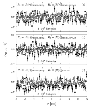
Figure 1: Relative differences in percentage, as given by Eq. (6), between the values of the quantity $R(r)$ obtained in different calculations, as a function of the distance to the source $r$ and for 80 keV photons. Panels (a) and (b) correspond to the two calculations performed with PENELOPE for $3\cdot 10^{7}$ and $3\cdot 10^{8}$ histories, respectively. Panel (c) corresponds to the difference between the first calculation with PENELOPE and the GEANT4 one for $3\cdot 10^{7}$ histories. Open circles (black squares) represent the results for which the value zero is (not) statistically compatible at the 1$\sigma$ level.

To illustrate a typical situation, we show in Fig. 1, the relative differences, $\Delta^{j}_{R_{1},R_{2}}$, in percentage, between the quantities $R(r)$ obtained in various calculations, as a function of $r$ and for 80 keV photons. Open circles (black squares) correspond to the bins for which the zero difference is (not) reached at the 1$\sigma$ level.

In panel (a) the two simulations compared have been performed with PENELOPE (v. 2003), but using two different seeds for the random number generator. A total of $3\cdot 10^{7}$ histories have been followed in this case. It is obvious that these two simulations must be identical. However, as we can see, there are some bins for which both calculations are compatible, but some of them are statistically different, even if the differences are really small (below $\sim$1%). Then, it is evident that, depending on the particular subset of bins selected, one could conclude that the agreement between the two calculations is almost perfect or exactly the opposite.

Increasing the number of histories does not solve the problem. In panel (b) we show the relative differences obtained in a similar situation to that plotted in panel (a), but following $3\cdot 10^{8}$ histories. We observe that the general trend is the same in both panels, the only difference being that now the values of $\Delta^{j}_{R_{1},R_{2}}$ are smaller when the number of histories increases. But, again, it is still possible to select a subset of individual bins for which the two simulations appear to be statistically different or very similar. Same situation is found if, instead of increasing the number of histories, the voxel volume is enhanced.

Finally, in panel (c) we compare two simulations done with PENELOPE (v. 2003) and GEANT4 for $3\cdot 10^{7}$ histories. Despite the fact that, now, two really different simulations are compared, the values obtained for $\Delta^{j}_{R_{1},R_{2}}$ are similar to those plotted in panel (a) and, as in the previous cases, one should conclude that both calculations are identical or completely different by adequately choosing particular bins for the comparison. However, in this particular case there is an additional fact to be taken into account: we observe a certain bias pointed out by the presence of a larger number of black squares with a negative value of the relative difference.

In order to avoid the possible errors linked to a restricted comparison between histograms, we propose to use a $\chi^{2}$-type statistic defined as

$$\chi^{2}_{H_{1},H_{2}}\,=\,\displaystyle\sum_{j=1}^{M}\frac{(H_{1}^{j}-H_{2}^{j})^{2}}{(\sigma_{1}^{j})^{2}+(\sigma_{2}^{j})^{2}}\,,$$ (7)

where $H_{1}^{j}$ and $H_{2}^{j}$ label the value in the $j$-th bin of the first and second histograms, respectively, and $\sigma_{1}^{j}$ and $\sigma_{2}^{j}$ are the corresponding uncertainties. One can state that two histograms are similar if $\chi^{2}_{H_{1},H_{2}}/M\sim 1$, $M$ being the number of degrees-of freedom (the number of histogram bins in our case). A value of $\chi^{2}_{H_{1},H_{2}}/M$ below 1 points out the presence of correlations between the quantities scored in the histograms. On the other hand, a value of $\chi^{2}_{H_{1},H_{2}}/M>1$ would indicate a discrepancy between the histograms (Frodesen et al., 1979; Press et al., 1992). The uncertainty of the quantity $\chi^{2}$ is given by $\sqrt{2\chi^{2}}$ (Frodesen et al., 1979). In the three cases considered in Fig. 1, the values of $\chi^{2}/M$ are 0.96$\pm$0.04, 0.97$\pm$0.04 and 1.39$\pm$0.05, respectively.

Besides, to estimate the significance of this $\chi^{2}$ test, we have used the standard chi-square probability function $Q(\chi^{2}|M)$ (Press et al., 1992). The smaller this probability is, the bigger the differences between the two histograms are. Following Press et al. (1992) we can state that if $Q\geq 0.1$ the agreement between both histograms is believable. If $0.001\leq Q<0.1$ the agreement is acceptable. Finally, if $Q<0.001$ both histograms have significant differences. In the two first cases shown in Fig. 1, the values of $Q(\chi^{2}|M)$ are 0.807 and 0.755, respectively. In the case of the comparison between PENELOPE and GEANT4 (panel (c)) this probability is 2.88$\cdot 10^{-15}$, much smaller than 0.001.

III Results

III.1 Comparison between PENELOPE (v. 2001) and (v. 2003).

Figure 2: Panel (a): Values of $\chi^{2}_{R_{1},R_{2}}/M$, as given by Eq. (7), calculated for the quantity $R(r)$, as a function of the energy of the initial photons. Panel (b): Relative differences in percentage, as given by Eq. (6), calculated for the same quantity, as a function of the distance to the source $r$ and for photons with initial energy of 1500 keV. The calculations compared have been done with the two versions of PENELOPE. The meaning of the open circles and the black squares in panel (b) is the same as in Fig. 1.

Before analyzing the obtained results, it is worth to point out that we have found small differences between the calculations performed with the two versions of PENELOPE. These differences appear mainly for the larger energies considered. This can be seen in panel (a) of Fig. 2 where the values of the $\chi^{2}_{R_{1},R_{2}}/M$, obtained for calculations done with PENELOPE versions 2003 ($R_{1}$) and 2001 ($R_{2}$) and with the phantom $\mathcal{P}_{\rm inf}$, are shown as a function of the initial photon energy. As we can see, the values of the quantity $\chi^{2}_{R_{1},R_{2}}/M$ obtained are close to 1, thus indicating the statistical consistency between the calculations performed with both versions of the code. The probabilities $Q(\chi^{2}|M)$ obtained are above 0.1 for all energies between 10 keV and 1 MeV, except for 60 and 250 keV where this probability is 0.06 in both cases. Above 1 MeV the two histograms show significant differences, the probabilities found being smaller than 0.001. In panel (b) of Fig. 2 we have plotted the relative differences, as given by Eq. (6), between the values of the quantity $R(r)$ obtained with the two versions of PENELOPE for an initial energy of 1.5 MeV. Therein the meaning of black squares and open circles is the same as in Fig. 1. As can be seen the discrepancy is mainly due to the first few bins of the corresponding histograms. In fact, if one does not consider the first bins for which the relative differences are larger than 1.5%, a probability $Q(\chi^{2}|M)>0.001$ is obtained.

The reason for these differences between both versions of the MC code PENELOPE can be ascribed to the modifications introduced in the version 2003 with respect to the 2001 one (Salvat et al., 2001, 2003): the X-ray energies are the experimental ones taken from Bearden (1967) (instead of being calculated as ionization energy differences as in the version 2001), the generalized oscillator strength model is fixed in order to reproduce the stopping powers quoted in ICRU (1984) and the inner-shell ionization by electron and positron impact is an independent process (which was not included in the version 2001). In what follows we use the version 2003 of PENELOPE only.

A few simulations performed, for some of the cases considered here, with the new versions 2005 and 2006 of the code have produced the same results as the version 2003.

III.2 Radial dose rate distributions

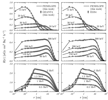
Figure 3: Comparison of the values of $R(r)$, as given by Eq. (2), obtained with PENELOPE (solid curves) with those calculated with GEANT4 (left panels) and with the results reported by Luxton and Jozsef (1999) with EGS4 (right panels). Various initial photon energies ranging from 15 keV to 2 MeV are plotted. Our calculations have been done with the ${\mathcal{P}}_{\rm inf}$ phantom. The uncertainties for the GEANT4 calculations are smaller than the size of the symbols used and those of the PENELOPE calculations are of the same order.

In this section we compare the results of our simulations with those obtained by Luxton and Jozsef (1999) and Ye et al. (2004). Fig. 3 shows the values of $R(r)$, as given by Eq. (2) for energies ranging between 15 keV and 2 MeV, as a function of the distance to the source, $r$, in the ${\mathcal{P}}_{\rm inf}$ phantom. In all panels, solid curves correspond to the simulations we have performed with PENELOPE. These are compared with the results obtained for GEANT4 (open squares) in left panels and with the results of the EGS4 simulation performed by Luxton and Jozsef (1999) (open circles) in right panels. An uncertainty of 1% was assumed for the data of these authors.

The results of PENELOPE and GEANT4 calculations agree rather well except at distances to the source smaller than 1 cm. Above 1 cm and for all energies, the differences between both calculations are below 1% of the maximum value of the corresponding $R(r)$.

At distances to the source smaller than 1 cm, the differences are, in general, larger. Below 0.5 cm and for energies smaller than 80 keV, the differences are bigger than 1% of the maximum of $R(r)$, reaching values around 3% of this maximum for the first bin (from 0 to 0.25 mm). In the energy range between 80 and 300 keV, only the first bin gives differences larger than 1% of the maximum value of $R(r)$. Above 300 keV, the differences are bigger than 2% of the maximum of $R(r)$ for distances to the source smaller than 0.5 cm. For the first bins, values around 8% of the maximum of $R(r)$ are found.

The differences between PENELOPE and EGS4 (Luxton and Jozsef 1999) follow the same trends for all the energies analyzed. At distances to the source above 1 cm, these differences are below 2% of the maximum of the corresponding $R(r)$. For distances smaller than 1 cm, the differences are at most 6% of the maximum of $R(r)$. Nevertheless, the first point available in the work of Luxton and Jozsef (1999) is $r=0.05$ cm and nothing can be said about distances closer to the source.

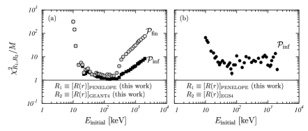
Figure 4: Values of $\chi^{2}_{R_{1},R_{2}}/M$, as given by Eq. (7), calculated for the quantity $R(r)$, as a function of the energy of the initial photons. The comparison between the results of our simulations with PENELOPE and GEANT4 are shown for the ${\mathcal{P}}_{\rm inf}$ (black squares) and ${\mathcal{P}}_{\rm fin}$ (open circles) phantoms in panel (a). In panel (b), we show the results for the comparison of our PENELOPE results with those of Luxton and Jozsef (1999) obtained with EGS4.

The degree of agreement between the different calculations can be evaluated by using the $\chi^{2}$ statistic defined in Eq. (7). In panel (a) of Fig. 4 we show with black squares the results obtained for the statistic when comparing the PENELOPE and GEANT4 results for the ${\mathcal{P}}_{\rm inf}$ phantom (plotted in left panels of Fig. 3). The $\chi^{2}/M$ appears to be rather large at low energies, close to 1 at medium energies and grows with energy above 200 keV. In these calculations of the $\chi^{2}$ statistic, the full histograms have been considered. In all cases the probability $Q(\chi^{2}|M)$ is smaller than 0.001.

In the same panel we have plotted the $\chi^{2}/M$ values obtained for the same comparison but using the ${\mathcal{P}}_{\rm fin}$ phantom. These values are practically the same as those previously discussed for energies below 50 keV. The reason for this behavior is that the finite phantom used is, in practice, infinite for these low energies. At higher energies, the $\chi^{2}/M$ values are larger for this finite phantom than for the infinite one. This is mainly due to the fact that the number of bins included in the calculations is smaller (roughly a factor 10) for ${\mathcal{P}}_{\rm fin}$: though the differences between PENELOPE and GEANT4 are similar for both phantoms, their relative importance is rather larger in the ${\mathcal{P}}_{\rm fin}$ case.

In panel (b) of Fig. 4, the results of the comparison between our PENELOPE simulations for the ${\mathcal{P}}_{\rm inf}$ phantom and the EGS4 calculations of Luxton and Jozsef (1999) are plotted. At low energy, the trend is similar to the one observed in the previous panel. In this case, values near $\chi^{2}/M\sim 1$ are not obtained. However, above 40 keV, the $\chi^{2}/M$ does not show the quick growth with energy found in the comparison between PENELOPE and GEANT4.

We have performed a comparison of our results with those of Ye et al. (2004) obtaining, as expected, a good agreement above 10 keV for the phantom ${\mathcal{P}}_{\rm fin}$). For 10 keV a certain discrepancy is observed which can be ascribed to the fact that these authors gave results for five bins only.

Apart from the random variability, we have not found any particular structure at 3 cm from the 2 MeV source, neither with PENELOPE nor with GEANT4 using both the ${\mathcal{P}}_{\rm fin}$ and the ${\mathcal{P}}_{\rm inf}$ phantoms. This supports the guess of Luxton and Jozsef (1999) and their observation was, probably, a simulation artifact.

The differences observed between the different calculations can be due to a variety of factors. For energies above a few hundred of keV, the disagreement found close to the source between PENELOPE and GEANT4 can be ascribed to the known problems of this last code with the multiple scattering implementation (Poon and Verhaegen, 2005), which affects the electron transport and is crucial in the absence of charged particle equilibrium, as it occurs precisely nearby the source. This is an important point because, as mentioned above, we have done calculations with GEANT4 using electron tracking parameters more exigent and we have found the same results.

For low energies, below 80 keV, electron transport is negligible and, at least in principle, the differences can be due only to the fact that the photoelectric and Compton cross sections used by the low-energy package of GEANT4 and PENELOPE are different. This discrepancy should be reduced by using the package PENELOPE of GEANT4, in which the same cross sections as in the PENELOPE code are used. As shown by Poon and Verhaegen (2005), the differences obtained for the photoelectric mass attenuation coefficient using the PENELOPE package and the low-energy package of GEANT4 are negligible. On the other hand, the differences for the Compton mass attenuation coefficient are smaller than 1.5% for energies below 200 keV. Above this energy, no differences are found. In order to see if these differences solve the discrepancies shown by our calculations, we have performed simulations using the PENELOPE package of GEANT4 for energies below 80 keV. First, we have found that these new results differ from those corresponding to the low-energy package by less than 1% of the maximum of $R(r)$ and, second, the modification does not improve the agreement with the results obtained with the PENELOPE code.

The differences observed between PENELOPE and EGS4 at low energies, where electron transport is not relevant, can be ascribed to the different cross sections used for photoelectric and Compton processes in both codes. Above 80 keV, also the differences in the electron tracking procedures used in these two codes affect. One can expect that EGSnrc (Kawrakow and Rogers, 2003), a newer version of EGS, with new implementations of the photoelectric and Compton process physics would reduce these differences to a large extent.

IV Conclusions

In this work, Monte Carlo codes PENELOPE and GEANT4 have been used to calculate the dose rate in water for monoenergetic photon point sources with energies of interest in brachytherapy, ranging between 10 keV and 2 MeV.

To compare the results obtained with these two codes between them and with those calculated by other authors, we have proposed a statistical test based on the evaluation of the $\chi^{2}$ between two histograms.

We have found some small discrepancies between the versions 2001 and 2003 of PENELOPE for source energies larger than 1 MeV, while the versions 2005 and 2006 provide results in perfect agreement with version 2003 in the cases here analyzed.

The comparison between PENELOPE and GEANT4 results shows a reasonable agreement for all energies analyzed except in the neighbor of the source, up to a few millimeters.

In the case of the infinite phantom, the PENELOPE results are also in reasonable agreement with previous EGS4 calculations of Luxton and Jozsef (1999) for distances larger than 1 cm.

The comparison of our results with the results of Ye et al. (2004) shows a good agreement above 10 keV for the finite phantom.

We have shown that the comparison between the histograms obtained as output of this kind of simulations can produce contradictory results if it is done on the basis of a restricted set of bins. To avoid this problem, at least in part, we have proposed a $\chi^{2}$ test which gives a quantitative estimate of the agreement or disagreement between histograms. However, due to its integral character, other relevant information can be lost (e.g., the possible bias, the bins which are actually different, etc.) Thus, further investigation to find additional statistics should be of interest in order to complete the analysis.

V ACKNOWLEDGMENTS

This work has been supported in part by the Junta de Andalucía (FQM0220) and by the Ministerio de Educación y Ciencia (FIS2005-03577). F.M.O. A.-D. acknowledges the University of Granada and the Departamento de Física Moderna for partially funding his stay in Granada (Spain).

References

- Agostinelli et al. (2003) Agostinelli, S., Allison, J., Amako., K., Apostolakis, J., et al., 2003. GEANT4 - A simulation toolkit Nucl. Instr. Meth. Phys. Res. A 506, 250-303
- Al-Dweri et al. (2004) Al-Dweri, F.M.O., Lallena, A.M., Vilches M., 2004. A simplified model of the source channel of the Leksell GammaKnife tested with PENELOPE. Phys. Med. Biol. 49, 2687-2703.
- Asenjo et al. (2002) Asenjo, J., Fernández-Varea, J.M., Sánchez-Reyes, A., 2002. Characterization of a high-dose rate 90Sr-90Y source for intravascular brachytherapy by using the Monte Carlo code PENELOPE. Phys. Med. Biol. 47, 697-711.
- Bearden (1967) Bearden, J.A., 1967. X-ray wavelengths. Rev. Mod. Phys. 39, 78-124.
- Berger (1968) Berger, M.J., 1968. Energy deposition in water by photons from point isotropic sources. J. Nucl. Med. Suppl. 1, 17-25.
- Cullen et al. (1997) Cullen, D.E., Hubbell, J.H., Kissel, L., 1997. EPDL97: The evaluated photon data library, ’97 version (LLNL Report UCRL-50400). (LLNL, Livermore)
- Frankle and Little (2000) Frankle, S.C., Little, R.C., 2000. Informal overview of the DLC-200/MCNPDATA package. (LANL, Los Alamos)
- Frodesen et al. (1979) Frodesen, A.G., Skjeggestad, O., Tofte, H., 1979. Probability and statistics in particle physics. (Universitetsforlaget, Bergen)
-
GEANT4 (2006)
GEANT4 Collaboration, 2006. Physics Reference Manual.
http://wwwasd.web.cern.ch/wwwasd/geant4/G4UsersDocuments/UsersGuides/ - ICRU (1984) ICRU 37, 1984. Stopping powers for electrons and positrons. (ICRU, Bethesda)
- Kawrakow and Rogers (2003) Kawrakow, I., Rogers, D.W.O., 2003. The EGSnrc code system: Monte Carlo simulation of electron and photon transport, NRCC Report PIRS-701 (NRC, Otawa), available at http://www.irs.inms.nrc.ca/inms/irs/EGSnrc/EGSnrc.html
- Luxton and Jozsef (1999) Luxton, G., Jozsef, G., 1999. Radial dose distribution, dose to water and dose rate constant for monoenergetic photon point sources from 10 keV to 2 MeV: EGS4 Monte Carlo model calculation. Med. Phys. 26, 2531-2538.
- Poon et al. (2005) Poon, E., Seuntjens, J., Verhaegen, F., 2005. Consistency test of the electron transport algorithm in the GEANT4 Monte Carlo code. Phys. Med. Biol. 50, 681-694.
- Poon and Verhaegen (2005) Poon, E., Verhaegen, F., 2005. Accuracy of the photon and electron physics in GEANT4 for radiotherapy applications. Med.Phys. 32, 1696-1711.
- Press et al. (1992) Press, W.H., Teukolsky, S.A., Vetterling, W.T., Flannery, B.P., 1992. Numerical recipes in Fortran77: The art of scientific computing. (Cambridge University Press, Cambridge)
- Sakamoto (1993) Sakamoto, Y., 1993. Photon cross section data PHOTX for PEGS4 code. Proc. Third EGS4 User’ Meeting in Japan. (KEK, Tsukuba)
- Salvat et al. (2001) Salvat, F., Fernández-Varea, J.M., Acosta, E., Sempau, J., 2001. PENELOPE - A code system for Monte Carlo simulation of electron and photon transport. (NEA-OECD, Paris)
- Salvat et al. (2003) Salvat, F., Fernández-Varea, J.M., Sempau, J., 2003. PENELOPE - A code system for Monte Carlo simulation of electron and photon transport (NEA-OECD, Paris)
- Sánchez-Reyes et al. (1998) Sánchez-Reyes, A., Tello, J.J., Guix, B., Salvat, F., 1998. Monte Carlo calculation of the dose distributions of two 106Ru eye applicators. Radiother. Oncol. 49, 191-196.
- Ye et al. (2004) Ye, S.-J., Brezzovich, I.A., Pareck, P., Naqvi, S.A., 2004. Benchmark of PENELOPE code for low-energy photon transport: dose comparisons with MCNP4 and EGS4. Phys. Med. Biol. 49, 387-397.