Autonomous detection and anticipation of
jam fronts from messages propagated by inter-vehicle communication

Abstract

In this paper, a minimalist, completely distributed freeway traffic information system is introduced. It involves an autonomous, vehicle-based jam front detection, the information transmission via inter-vehicle communication, and the forecast of the spatial position of jam fronts by reconstructing the spatiotemporal traffic situation based on the transmitted information. The whole system is simulated with an integrated traffic simulator, that is based on a realistic microscopic traffic model for longitudinal movements and lane changes. The function of its communication module has been explicitly validated by comparing the simulation results with analytical calculations. By means of simulations, we show that the algorithms for a congestion-front recognition, message transmission, and processing predict reliably the existence and position of jam fronts for vehicle equipment rates as low as 3%. A reliable mode of operation already for small market penetrations is crucial for the successful introduction of inter-vehicle communication. The short-term prediction of jam fronts is not only useful for the driver, but is essential for enhancing road safety and road capacity by intelligent adaptive cruise control systems.

1 Introduction

Inter-vehicle communication (IVC) is widely regarded as a promising concept for transmitting traffic-related information. There are essentially two types of future applications that inspire the research on IVC: Applications in traffic safety such as automated reaction to an emergency incident, cooperative, autonomous driving and platoon formation on freeways rely on fast communication and information transmission between single vehicles (Varaiya, 1993; Rao et al., 1993; Rao and Varaiya, 1993; Aoki and Fujii, 1996; Tank and Linnartz, 1997). On the other hand, applications towards advanced traveler information systems, dynamic routing, or entertainment applications do not depend critically on information transmission times.

Recently, another application field of IVC has been proposed in the context of strategically operating adaptive cruise control (ACC) systems that change their driving characteristics automatically on an intermediate timescale according to the local traffic situation (Kesting et al., 2007b). While currently available ACC systems aim to enhance the comfort and safety of driving, their impact on the capacity and the stability of traffic flow on freeways has moved into the focus of traffic research (Kesting et al., 2006; Davis, 2004; VanderWerf et al., 2001; Treiber and Helbing, 2001; Marsden et al., 2001). Receiving traffic-related messages via IVC could help ACC systems to recognize relevant traffic situations faster and more reliably. This allows ACC-equipped vehicles to drive with an ’intelligent’ driving strategy that adapts the ACC parameters to the current traffic situation thereby changing the ’driving style’. For example, if the positions of jam fronts were known in advance, an ACC system could brake earlier and smoother when approaching the upstream jam front to increase traffic safety. In contrast, it could keep smaller time gaps to the leader when leaving the jam at the downstream jam front to increase the jam outflow (discharge rate), while staying at a normal operation characteristics in all other situations. Furthermore, ACC-equipped cars acting as ’floating cars’ are also able to detect the position of jam fronts and, consequently, may spread such information via IVC. However, as IVC will start on the basis of a small number of equipped vehicles, it is crucial to investigate the functionality and the statistical properties of the message hopping processes under such conditions. These questions have been investigated recently within the German research project INVENT (BMBF, 2005).

Fast and reliable information spreading is a necessary precondition for a successful implementation of all mentioned IVC-based applications. Assuming a sufficient market penetration, IVC offers the possibility of a decentralized and robust traffic information system, where the data is collected, evaluated, and distributed autonomously by each single car. Note, that estimations of the necessary market penetration for IVC depend on the application, that means on the type of information that is transmitted and how this information is used. The transmission of messages within a dynamic ad-hoc network of vehicles has been investigated on different levels of abstraction with respect to protocol design (Kim and Nakagawa, 1997; Xu et al., 2004) and message propagation efficiency. The latter aspect that is also addressed in this contribution has been investigated by simulations and by analytical calculations in different studies (Briesemeister et al., 2000; Wischhof et al., 2005; Wu et al., 2004, 2005; Jin and Recker, 2006). We refer to Yang and Recker (2005) for a short and thorough literature overview.

In this contribution, we present an IVC-based application of vehicle-based jam-front detection and prediction. By means of a microscopic traffic simulation, we simulate the whole chain of information generation, transmission, and interpretation based on a small fraction of vehicles equipped with IVC. Single vehicles in the traffic simulation detect jam fronts and generate traffic-related messages based on their locally available floating-car data. These messages are propagated further upstream via IVC mainly by cars of the opposite driving direction. Finally, the received information is used for a reconstruction and short-term prediction of the expected traffic situation further downstream which can serve as basis for determining the appropriate ACC strategy as discussed by Kesting et al. (2007b). We will investigate the prediction error for an equipped car as a function of the distance to the predicted jam front. Notice that this individual short-term traffic forecast is of general interest for the driver.

Our paper is structured as follows: In Sec. 2, we introduce the model of IVC and the generation of traffic-related messages based on floating-car data. In Sec. 3, the properties of the simulated message transmissions are validated by comparison to analytical calculations. We also discuss the IVC parameters. In Sec. 4, the proposed algorithm for detecting and predicting jam fronts is applied to a basic traffic scenario. Finally, we conclude with a short discussion and an outlook.

2 Microscopic modeling of inter-vehicle communication and message generation

2.1 Characteristics of inter-vehicle communication and its implementation

In this section, the model of inter-vehicle communication (IVC) is introduced. In the context of freeway traffic, messages have to travel upstream in order to be valuable for their receivers. In general, there are two strategies, how a message can be transported upstream via IVC as displayed in Fig. 1: Either the message hops from one IVC car to a subsequent IVC car within the same driving direction (’longitudinal hopping’), or the message hops to an IVC-equipped vehicle of the other driving direction, which takes the message upstream and delivers it back to cars of the original driving direction (’transversal hopping’).

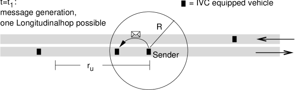
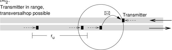
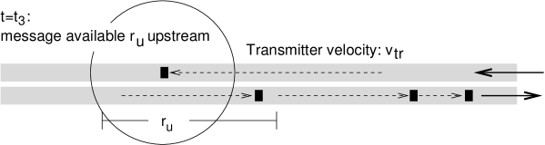
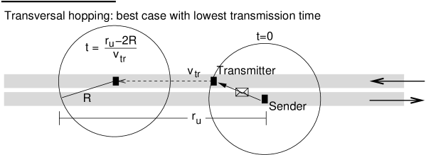
Figure 1: Basic mechanisms for the transport of a traffic-related message on a freeway: The sender (e.g., having recognized an upstream jam front) generates a message and starts broadcasting it. The message may be received by a subsequent car via a longitudinal hop. At time $t_{2}$, the message is received by an equipped transmitter car via a transversal hop. The characteristic quantity of the communication process is the time $\tau=t_{3}-t_{1}$ from the message generation until it is available for the first time at a user distance $r_{\text{u}}$ upstream of the position where the message has been generated. The minimal time $\tau$ for transversal hopping is realized for a configuration as shown in the last sketch: The transmitter (velocity $v_{\text{tr}}$) must be at the optimal position at $t=0$, i.e., a distance $R$ upstream of the sender. The message is available, when the transmitter has covered the distance $r_{\rm u}-2R$, i.e., after a time $\tau_{\rm min}=(r_{\rm u}-2R)/v_{\rm tr}$. Notice that only IVC-equipped vehicles are depicted in the illustrations.

For a low density of equipped cars, i.e., for a small market penetration, an instantaneous multiple longitudinal hopping is not very likely due to gaps that are larger than a given limited broadcast range (Dousse et al., 2002). It is argued, that the gaps in multi-lane traffic may be bridged after a while because of different velocities of the equipped cars. However, this is a minor effect: For low densities of equipped vehicles, a message propagates in driving direction just with the velocity not larger than the velocity of the fastest cars (Wu et al., 2004). Therefore, we conclude that the longitudinal hopping against the driving direction does not work for low densities of equipped vehicles, because the mechanism for bridging gaps is to slow for a real backward propagation of the messages – the normal downstream movements of messages inside the cars cannot be outmatched by the wireless communication in upstream direction. Thus, longitudinal hopping will only have some impact in combination with transversal hopping in order to enhance the message propagation in the traffic stream of the opposite driving direction. However, in case of dense traffic conditions (which is to be distinguished from a high density of IVC-equipped vehicles), the variation in the velocities of the vehicles is limited. As a consequence, even in the limit of long timescales, the obtained propagation velocity is similar to the mean velocity of the transmitter vehicles (Wu et al., 2004).

In the following, the used microscopic model for the IVC-related processes is outlined: Every 2 seconds, messages are exchanged between IVC-equipped vehicles within a limited broadcast range $R$. Each car sends all its stored messages, and the default broadcast range is set to $250\,$m. These assumptions are well justified with regard to the current technological possibilities of data exchange between vehicles, cf. the next Sec. 2.2. Furthermore, we neglect the width of the road in the calculations and simulations, i.e., the broadcast range $R$ refers to the longitudinal distances.

Because of the low efficiency of longitudinal hopping, we restrict ourselves to transversal hopping processes. Each car accepts only messages from the other driving direction, either as a transmitter vehicle (after the first transversal hop), or as a user that receives information about its own driving direction (after a second transversal hop). All other messages will be discarded directly after reception. Furthermore, messages related to events at an already passed position, and messages that are older than 10 minutes are deleted as well. As the routing in this system is obviously given by the two traffic streams in opposite directions, no further rule is necessary for modeling the message exchange process.

2.2 Technological basis for inter-vehicle communication

The assumptions about the exchange of small traffic-related data packages are justified by the experimentally proven possibilities of data transmission between vehicles on the freeway within the IEEE 802.11b standard. Operating WLAN equipment on a freeway with an external antenna in a broadcast-like modus, i.e., using IP/UDP (user datagram protocol), allows a data throughput of about 1Mb/s. This holds for distances of about 300m, and even for cars moving in different driving directions with a relative speed difference of 200 km/h (Singh et al., 2002). Despite high relative velocity differences between two vehicles, the total transmission of more than three MB data within one encounter has been reported (Ott and Kutscher, 2004), although the available time within the broadcast range decreases with the relative velocity, and some time is needed to associate to the communication channel. Without giving quantitative values, Günter and Großmann (2005) predict for a high vehicle density and for a high market penetration rate a breakdown of of the communication due to too many users using the available bandwidth. Such scenarios indeed have not yet been investigated empirically. The reduction of transmission power, or simply sending messages more rarely may avoid the breakdown of the communication channel: For the jam front prediction, it is not necessary to receive a message of every single car, that has detected the front. In addition, the new pending standard IEEE 802.11p, for “Wireless Access for the Vehicular Environment” comes with a much more fast and efficient protocol than the IP protocol: The “Dedicated Short Range Communications” (DSRC) is a concept specifically designed for automotive use. According to Xu et al. (2004), i.e., it is no problem to transmit in normal freeway traffic (4 lanes, 33veh/km/lane) small data packages of 400 Bytes from each car to each other car inside a broadcast range of 150 m within a fraction of a second, and with a loss rate of below 1%. Notice, that a message containing traffic-related information, i.e., about a jam front, has a size of the order of a few hundred Bytes rather than Kilobytes.

2.3 Congestion fronts: Recognition and generation of traffic-related messages

Since our focus is to use the traffic information as input for traffic-adaptive ACC systems, the crucial events to be detected and transmitted are the positions of jam fronts.

There are cases, when an (expected) jam front position may be anticipated, e.g., if a car got stuck into a traffic jam upstream bottleneck, that is well-known for causing congestion. In many cases, jam front positions can only be exactly detected by cars passing the location. Figure 2 illustrates three examples of different congestion fronts:

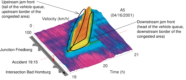
Figure 2: Example for the spatiotemporal dynamics of freeway jams for illustrating different types of jam fronts (see the main text). This traffic jam on the German freeway A5 between Kassel and Frankfurt in direction South was caused by a blockage of the most-right of altogether three lanes after an accident occurred as noted in the sketch of the freeway. 1-minute averaged date of the velocity had been recorded by double loop detectors with an average distance of 1 km. The shown velocity field has been obtained by using an adaptive smoothing method for interpolation of macroscopic traffic data between the detectors (Treiber and Helbing, 2002). The driving direction of the cars is indicated by the black arrow. Notice the inverted vertical axis for matters of better illustration.

1. A downstream jam front is pinned at some bottleneck, e.g., at the location of an incident referring to the straight line in Fig. 2.

2. A downstream jam front (a dissolution front of congested traffic) is propagating against the traffic flow with a characteristic speed of about $-15\,$km/h (Kerner and Rehborn, 1996; Helbing et al., 1999; Schönhof and Helbing, 2004).

3. An upstream jam front is moving with an propagation speed that depends on the traffic flow upstream of the jam and the flow in the jam.

Downstream jam fronts are normally straight lines in the spatiotemporal plane. These fronts either are fixed at a bottleneck, or move with a constant velocity of approximately -15 km/h – apart from few cases of a ’moving bottleneck’ where the propagation velocity can assume other values but is constant as well. This fundamental feature of traffic flow dynamics is found in most of the empirical work and is also reflected in the traffic models from the very beginning (Lighthill and Whitham, 1955). The velocity of downstream jam fronts can even be constant for hours. For stationary inflow conditions, upstream jam fronts also have a constant velocity. It may vary between between -25 km/h (the high value of -40 km/h reported by Bertini and Malik (2004) has not been observed in other studies), and the velocity of freely driving vehicles (if the inflow is vanishing and a cluster of vehicles is accelerating). In the most cases, the approximation of a constant front velocity is justified, because the traffic demand normally does not change significantly on time scales of 5–10 minutes.

For the detection and prediction of jam fronts, their spatial extension has to be considered (Muñoz and Daganzo, 2003). Due to the discrete nature of traffic, the jam ’front position’ as a continuous line in time and space can only be thought as an abstract result of an averaging process based on vehicle trajectories.

In the following, a model for the jam front detection based on floating-car data is presented: The jam front is characterized by the time and the location, when a passing car starts to brake or to accelerate. In order to reliably detect these acceleration and deceleration processes, and to minimize the number of ’false alarms’, each car smoothes its floating-car data, i.e., its velocity $v(t)$ using an exponential moving average (EMA):

$$v_{\text{EMA}}(t)=\frac{1}{\tau}\int\limits^{t}_{-\infty}dt^{\prime}e^{-(t-t^{\prime})/\tau}\,v(t^{\prime}),$$ (1)

with a relaxation time $\tau=10$ s. The EMA allows for an efficient real-time update by using an explicit integration scheme for the corresponding ordinary differential equation

$$\frac{d}{dt}v_{\text{EMA}}=\frac{v-v_{\text{EMA}}}{\tau}.$$ (2)

The detection of an upstream or downstream jam front relies on a change in speed compared to the exponentially averaged past of the speed. An upstream jam front is therefore given, when for the first time

$$v(t)-v_{\text{EMA}}(t)<-\Delta v_{\text{up}}$$ (3)

holds, with $\Delta v_{\text{up}}=15$ km/h. A downstream jam front is identified by the first notice of an acceleration period,

$$v(t)-v_{\text{EMA}}(t)>\Delta v_{\text{down}}.$$ (4)

with $\Delta v_{\text{down}}=10\,$km/h. When a congestion front is detected, a corresponding message containing position, time, and jam-front type is generated. This message is repeatedly broadcasted until it is discarded after 10 minutes.

3 Statistics of message propagation via the opposite driving direction

In this section, we will compare simulation results for the efficiency of IVC via transversal hopping with analytical results (Schönhof et al., 2006). Moreover, we will shortly discuss the parameters of the system.

When the proportion $\alpha$ of vehicles equipped with IVC is low, the positions of the IVC-equipped cars can be assumed to be statistically independent of each other. Therefore, the arrival process of an equipped vehicle at a given cross-section is a Poisson process. This holds even for high traffic densities, where the positions of neighboring vehicles are highly correlated. We define the density of equipped cars $\lambda$ in one driving direction by $\lambda=\rho\alpha$, where $\rho$ is the traffic density over all lanes. As a consequence of the Poisson process, the longitudinal distances $\Delta$ between consecutive equipped are exponentially distributed with the probability density

$$f(\Delta)=\lambda e^{-\lambda\Delta},$$ (5)

which is very well supported by empirical data (Schönhof et al., 2006).

Particularly, given the full density $\lambda_{\rm tr}$ of equipped cars on all lanes for the opposite driving direction, we may calculate the cumulative probability distribution of the time $\tau$, after which the message is available at the distance $r_{\rm u}$ upstream from the position of message generation:

$$P(\tau<t)=\Theta\left(t-\frac{r_{\rm u}-2R}{v_{\rm tr}}\right)\left(1-e^{-\lambda_{\rm tr}\left(2R+v_{\rm tr}t-r_{\rm u}\right)}\right).$$ (6)

Here, $R$ denotes the broadcast range of a sender/receiver unit, $v_{\rm tr}$ is the (average) velocity on the opposite lanes, and the Heavyside function $\Theta(x)$ is defined by $\Theta(x)=1$ for $x>0$ and $\Theta(x)=0$ otherwise.

The left diagram in Fig. 3 shows the distributions of $\tau$ for several values of $\alpha$. The microscopic simulation approach allows for a detailed modeling of the message broadcast and receipt mechanisms of IVC equipped vehicles (cf. Fig. 4). For a description of the traffic simulation setup cf. the beginning of Section 4.1. To obtain the statistics of message propagation, the equipped vehicles have generated a ’dummy’ message while crossing the position $x=5\,$km in a freeway stretch of $10\,$km length, and the cycle time for the communication has been set to $0.5\,$s. The results show a very good agreement with the analytical calculations (Eq. 6). Note that the lower limit for $\tau$,

$$\tau_{\rm min}=\frac{r_{\rm u}-2R}{v_{\rm tr}}\,,$$ (7)

is realized, if the transmitter has an optimal position at $t=0$, cf. Fig. 1.

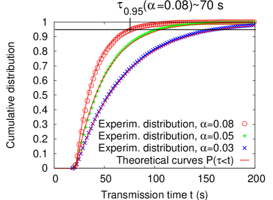
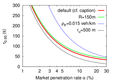
Figure 3: Left diagram: Cumulative distribution of transmission times, if messages are transmitted via cars in the opposite driving direction. Symbols correspond to simulation results and solid curves to the analytical result of Eq. (10). The assumed IVC parameters are the broadcast range $r_{\rm max}=250\,$m and the minimal delivery range $r_{\rm u}=1000\,$m. A chosen moderate inflow of $Q=1240$/h/lane resulted in a transmitter-vehicle velocity of $v_{\rm tr}=85\,$km/h and an overall traffic density of $\rho=29$/km in each direction. The simulations have been carried out with equipment rates of $\alpha=3$%, $\alpha=5$%, and $\alpha=8$%. With rising market penetration rate $\alpha$ the message transport becomes faster. The time $\tau_{0.95}$ indicates when 95% of the messages are available $r_{\rm u}=1000\,$m upstream.
Right diagram: Investigation, how the efficiency of the message propagation in terms of $\tau_{0.95}$ depends on the parameters by evaluating Eq. 10. The default parameters are $r_{\rm u}=1000\,{\rm m}$, $r_{\rm max}=250\,{\rm m}$, $\rho=0.03/{\rm m}$ and $v_{\rm tr}=90\,{\rm km/h}$. Each of the other curves result by the variation of only one parameter, which reveals its impact.

Apart from this lower limit, which depends on $R$, $r_{\rm u}$, and $v_{\rm tr}$, the value of $P(\tau<t)$ is strongly influenced by the density of equipped vehicles in the opposite driving direction. This becomes obvious, by looking at the expectation value $\langle\tau\rangle$:

$$\langle\tau\rangle=\frac{r_{\rm u}-2R}{v_{\rm tr}}+\frac{1}{\lambda_{\rm tr}v_{\rm tr}}.$$ (8)

The higher the market penetration level $\alpha$, the higher are the values for $\lambda_{\rm tr}=\alpha\rho_{\rm tr}$, and the earlier a message arrives upstream due to the decreasing second part of the expression for $\langle\tau\rangle$ (the average waiting time for a transmitter car).

Let us now consider the $95$th percentile of the IVC transmission time as a quantity for the IVC efficiency. The definition

$$P(\tau\leq\tau_{0.95})=0.95$$ (9)

leads to the result

$$\tau_{0.95}=\frac{r_{\rm u}-2R}{v_{\rm tr}}+\frac{\ln(\frac{1}{0.05})}{\lambda_{\rm tr}v_{\rm tr}}.$$ (10)

This quantity is shown in Fig. 3 (right) for four different scenarios. For a low equipment rate $\alpha$, it depends only weakly on the broadcast range $R$ and the minimal propagation distance $r_{\rm u}$, because the second term in Eq. (10) dominates: The traffic density $\rho_{\rm tr}$ on the opposite lanes has a high impact.

Notice that in the limit of the upstream distance $r_{\rm u}\to\infty$, the mean IVC propagation velocity $\langle v\rangle=\langle\frac{r_{\rm u}}{\tau}\rangle$ converges to $v_{\rm tr}$, i.e., to the average speed of the vehicles. So, at least in the long term, messages can propagate faster via the transversal hopping mechanism than any congestion front because the maximum upstream propagation of jam fronts is much smaller than $v_{\text{tr}}$ (Bertini and Malik, 2004).

4 Simulation of jam-front detection and prediction

4.1 Traffic simulation scenario

For matters of illustration, we apply the proposed jam-front detection (Sec. 2.3) and the message propagation via IVC (Sec. 3) to a specific traffic scenario.

As simulation scenario, we consider a homogeneous freeway section of length $5\,$km with two independent driving directions and altogether four lanes. The longitudinal movement of the vehicles are described by the Intelligent Driver Model (IDM) (Treiber et al., 2000), which is a simple and realistic car-following model. The lane-changing decision are based on the recently proposed model MOBIL (Kesting et al., 2007a). We have introduced heterogeneity by distributing the desired velocities of the ’vehicle-driver units’ according to a Gaussian distribution with a standard deviation of $18\,$km/h around a mean speed of $v_{0}=120$ km/h. The other parameter values have been chosen according to Kesting et al. (2006). Notice that the details of the traffic model do not influence the dynamics of message propagation via IVC, which is our main focus here.

A given fraction $\alpha$ of the cars is randomly chosen to be equipped with an IVC module. In the simulation, these vehicles determine additionally their position by a ’satellite positioning system’ and feed their ’jam front detection device’ by their own velocity time series according to Sec. 2.3.

In one driving direction, we have triggered a stop-and-go wave (’Moving Localized Cluster’, (Helbing et al., 1999; Schönhof and Helbing, 2004)), while traffic is free in the other driving direction. The inflow at both upstream boundaries of the simulated freeway stretch is set to $1800\,$vehicles/h/lane. Notice that the outflow (discharge rate) at the downstream jam front is of the same order, so that the upstream and the downstream jam front propagate with the characteristic speed of about $15\,$km/h in upstream direction through the system.

We consider an IVC equipment rate of $\alpha=3$%. The resulting trajectories and the sending and receiving events via transversal hopping are illustrated in Fig. 4. As already pointed out in Sec. 2.1, the distance of the equipped vehicles often exceeds the broadcast range of $R=250\,$m, even in the region of congested traffic. As shown in Fig. 4, the considered vehicle receives the first message about the upcoming traffic congestion already $2\,$km before encountering the traffic jam. Further received messages from other equipped vehicles are used to confirm and update the predicted downstream traffic situation.

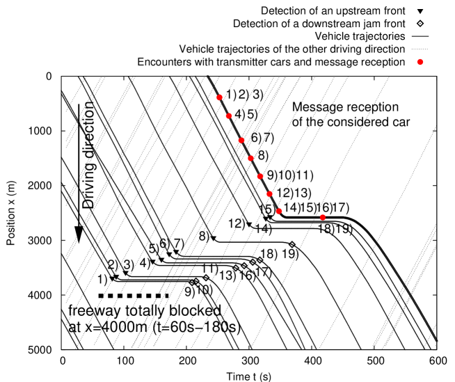
Figure 4: Space-time diagram of the considered traffic scenario. The trajectories of IVC-equipped vehicles (only 3% of all vehicles) are displayed by solid and dotted lines depending on the driving direction. The vehicles in the other driving direction serve as transmitter cars for the transversal hopping mechanism. A temporary road blockage triggers a stop-and-go wave indicated by horizontal trajectory curves in one driving direction. When cars encounter the propagating ’moving localized cluster’, they broadcast messages about the detected position and time of the upstream jam front and the following downstream jam front. These message generations are represented by numbers. The reception of these messages by the considered vehicle (thick solid line) is indicated by the same numbers. The trajectories of the subsequent vehicles of this considered car are not shown. Notice that the crossing trajectories of equipped vehicles in the upper-left corner in the diagram refer to a passing maneuver due to different desired velocities

4.2 Interpretation of the received messages: Jam front prediction algorithm

After the generation and propagation of traffic-related messages, the received messages are finally used for a vehicle-based reconstruction and prediction of the downstream traffic situation. Each car in the microscopic simulation sorts the incoming messages according to the reported jam-front type for a separate evaluation. Within each message group, all messages that are not older than 120 s (compared to the most recently received message) are considered for the prediction: If this selection process yields two or more relevant messages, the prediction for the jam front is based on linear regression in the space-time plane, as the assumption of a constant jam front velocity is well justified for the time scale of several minutes, cf. Sec. 2.3. In case of only one valid message, the reported position in this message is regarded as the prediction of the jam front position.

In order to analyze the quality of the jam-front prediction, we define an error measure that compares the prediction calculated at a time $t_{\text{p}r}$ with the actual realization of the jam front. Notice that this error can only be calculated a posteriori as the considered vehicle will pass the real jam-front at some time in the future. As the forecast is carried out autonomously by each equipped vehicle, we now consider a single car $c$ with its trajectory $x^{c}(t)$. At a considered time $t_{\text{pr}}<t$, the car is located at $x^{c}(t_{\text{pr}})$ and predicts the position of the jam front at time $t$ by the linear regression function $X_{\text{fr}}^{c\,,\,t_{\text{pr}}}(t)$. The prediction quality is evaluated ex post when the vehicle $c$ detects itself the jam front at a time $t_{\text{fr}}^{c}$ and at a position $x^{c}(t_{\text{fr}}^{c})$. Thus, the difference between the real jam-front position $x^{c}(t_{\text{fr}}^{c})$ and the predicted one for the time $t_{\text{fr}}^{c}$ defines the error $e$ by

$$e^{c}(t_{\text{pr}})=x^{c}(t_{\text{fr}}^{c})-X_{\text{fr}}^{c\,,\,t_{\text{pr}}}\left(t_{\text{fr}}^{c}\right).$$ (11)

Figure 5 illustrates the error $e$ for two snapshots at the prediction times $t_{\text{pr}}=260\,$s and $340\,$s, respectively. As shown in the diagrams, $e$ decreases when approaching the jam-front as measured by the distance $D$.

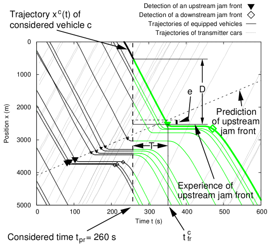
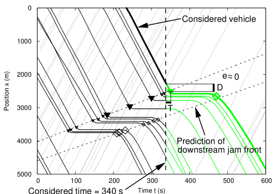
Figure 5: Two subsequent snapshots of our congestion front prediction as the considered vehicle (thick solid line) approaches the jam front. The symbols denote the generation of messages when a vehicle detects a jam front. Messages indicated by large symbols are used for the actual jam front prediction by the considered car, while small symbols correspond to outdated messages or messages that have not yet reached the considered car via IVC. The prediction quality is measured by the error $e$, which is defined by the difference between the real jam-front position as it will be detected by the considered car in the future and the actually predicted position for this event at a given time. Notice that the error $e$ can only be calculated a posteriori as it compares prediction and realization.

Each equipped car predicts the jam fronts every two seconds according to the communication cycle described in Sec. 2.1. If no messages arrive in one update cycle, no new prediction will be estimated. After the simulation run, we determine the prediction error $e$ ’off-line’. The prediction error $e$ (Eq. 11) depends on the time $t_{\text{pr}}$ and should, in average, decreases when the considered car approaches the predicted jam front due to the reception of new messages allowing for a better forecast. By a simple time shift transformation,

$$T:=t_{\text{fr}}^{c}-t_{\text{pr}},$$ (12)

$e$ depends on the time interval $T$ between the prediction time and the time when the traffic jam front is reached.

In Fig. 6 all single predictions in each car for a scenario of Fig. 5 are shown. For matters of illustration, the subsequent predictions of a single car are connected by dotted lines. In Fig. 6(a,b), it is shown, how the error $e$ for the upstream jam front prediction depends on $D$ and $T$. In the case $D\to 0$ corresponding to $T\to 0$, the final deviations $e$ of the considered vehicles do not exceed an interval of about $\pm 50\,$m. The two diagrams show similar characteristics because the velocity of the cars does not vary significantly so that $D$ is essentially proportional to $T$.

Notice that this does not hold anymore when approaching a downstream jam front as shown in Fig. 6(c,d). A considered car spends approximately $120\,$s in the jam, and, as a consequence, is already close to the downstream jam front. Therefore, the car receives several messages and updates predictions for $D\approx 50\,$m. This explains the clustering of the symbols in Fig. 6(c), while this effect is not relevant in the representation of Fig. 6(d). In the latter diagram, it can be seen, that for a car in the congestion zone ($T<120$ s) the mean frequency of prediction changes is decreased compared to the situation in the free flow state because a non-moving vehicle encounters less frequently transmitter cars of the other driving direction and thus receives less new messages per time than a moving vehicle. For $T\to 0$, the errors for predicting the downstream jam front are restricted to values of the order of $\pm 100\,$m. It turned out, that the reason is given by the characteristics of the downstream jam front. As visible in Fig. 5 and Fig. 4, the downstream jam front becomes smoother after some time – the cars spend more time (and space) in the acceleration process. This is due to the traffic dynamics in this special situation. The first car leaving the jam has no leader car in front, and thus its acceleration is higher compared to subsequent cars leaving the jam. This affects the detection of the front, which gets more and more delayed compared to the first detection processes at $t=200$ s. Thus the prediction of the front position is likely to be further upstream than the actual position detected according to Eq. (4), which leads to prediction errors of $e>0$ according to applied definition of $e$. The second clustering of $e$ in the interval between 50 and 100 m seems to be a result of this spatiotemporal curvature of the jam front. In summary, it has to be stated, that the prediction errors are also caused by uncertainties in determining the actual position of the downstream front by Eq. (4).

Figure 6: The prediction errors $e$ of several equipped cars for the upstream jam front (a,b) and the downstream jam front (c,d) for the traffic scenario shown in Fig. 5. In order to guide the eyes, subsequent predictions of an equipped car are connected by a dotted line. The prediction (and, thus, the prediction error) is updated when a car gets new messages via inter-vehicle communication. The diagrams show the errors as a function of the spatial distance $D$ to the real jam front position in the future (a,c) and as a function of the remaining time $T$ (b,d). The errors decrease with decreasing $D$ and $T$ as the vehicles approach the jam fronts. For $e>0$, the predicted jam front position is further upstream than the real jam front, cf. Fig. 5.

5 Summary, critical discussion, and outlook

In this contribution, a completely distributed freeway traffic information system based on inter-vehicle communication (IVC) has been introduced. It involves an autonomous, vehicle-based jam front detection, the information transmission via IVC, and the prediction of the spatial position of jam fronts by reconstructing the spatiotemporal traffic situation based on the transmitted information. The whole system is simulated within an integrated microscopic traffic simulation framework. The function of its communication module has been explicitly validated by comparing the simulation results with analytical calculations for the message propagation. By means of simulations, we have shown that the algorithms for a congestion-front recognition, message transmission, and processing predict reliably the existence and position of jam fronts for vehicle equipment rates as low as 3%. The prediction error decreases when a car is approaching the front, but does not go to zero due to uncertainties in determining the exact positions of a jam front. Notice that a reliable mode of operation for small market penetrations is crucial for the successful introduction of the technology proposed in this paper. The obtained accurate prediction results can be used as (non-local) input for a traffic-adaptive ACC system that changes its driving characteristics according to the local traffic situation as recently proposed by Kesting et al. (2007b). Furthermore, the timely knowledge about the upcoming traffic situation on a scale of minutes and a few kilometers offers new possibilities for vehicle-based advanced driver information systems.

Our feasibility study has been based on the following main assumptions and mechanisms: (i) Inter-vehicle communication allows for a reliable exchange of small data packages between vehicles in different driving directions with speed difference of up to $300\,$km/h. The broadcast range is limited, e.g., to $250\,$m. (ii) Traffic in the opposite driving direction is free. In the traffic simulations, stationary traffic flow conditions have been assumed, but this is not a precondition for the functionality of the proposed concept. (iii) The propagation speed of the dynamic jam fronts changes little on time scales of several minutes.

A few short remarks concerning the presented approach may summarize the limitations of our study. The currently available communication technology, and the future standards of wireless data transmission between vehicles, allow for a fast and reliable dissemination of small traffic-related messages (as needed for our concept) even for a high density of equipped vehicles. However, it should be mentioned that other applications may use the provided bandwidth as well. We suppose that there will be a balanced distribution of the resources needed for traffic safety, traffic information, and other applications.

For a small market penetration of IVC-equipped vehicles, the characteristics and efficiency of the message transport rely to a large extend on the density of equipped vehicles of the opposite driving direction and their driving speed. Note, that in rush hours, often only one of the driving directions is congested. The same applies for traffic congestion caused by accidents. Thus in most of the cases, free traffic flow of the opposite driving direction can be assumed. With respect to the considered application in ’traffic-adaptive’ ACC systems, it is essential to predict traffic-jam fronts. Within short time scales of 5 to 10 minutes, the velocity of the traffic-jam fronts can be assumed to be constant in the most cases, in particular for downstream jam fronts. Further research is necessary in order to improve the proposed prediction model and to reduce the prediction error. In particular, this applies to traffic situations with several traffic jam fronts of the same type and to special situations, in which the jam-front velocity changes, e.g., because of the clearance after an accident.

References

- Aoki and Fujii (1996) Aoki, M., Fujii, H., 1996. Inter-vehicle communication: technical issues on vehicle control application. Communications Magazine, IEEE 34, 90–93.
- Bertini and Malik (2004) Bertini, R. L., Malik, S., 2004. Observed dynamic traffic features on freeway section with merges and diverges. In: Transportation Research Record: Journal of the Transportation Research Board. Vol. 1867. Transportation Research Board of the National Academies, pp. 25–35.
- BMBF (2005) BMBF, 2005. Research project INVENT – Intelligent Traffic and User-Friendly Technology. http://www.invent-online.de.
- Briesemeister et al. (2000) Briesemeister, L., Schäfers, L., Hommel, G., 2000. Disseminating messages among highly mobile hosts based on inter-vehicle communication. In: IEEE Intelligent Vehicles Symposium. pp. 522–527.
- Davis (2004) Davis, L., 2004. Effect of adaptive cruise control systems on traffic flow. Phys. Rev. E 69, 066110.
- Dousse et al. (2002) Dousse, O., Thiran, P., Hasler, M., 2002. Connectivity in ad-hoc and hybrid networks. In: IEEE Infocom 2002. pp. 1079–1088.
- Günter and Großmann (2005) Günter, Y., Großmann, H. P., 2005. Usage of wireless LAN for inter-vehicle communication. In: IEEE Intelligent Transportation Systems Conference. pp. 408– 413.
- Helbing et al. (1999) Helbing, D., Hennecke, A., Treiber, M., 1999. Phase diagram of traffic states in the presence of inhomogeneities. Phys. Rev. Lett. 82, 4360–4363.
- Jin and Recker (2006) Jin, W.-L., Recker, W. W., 2006. Instantaneous information propagation in a traffic stream through inter-vehicle communicationn. Transportation Research Part B 40, 230–250.
- Kerner and Rehborn (1996) Kerner, B., Rehborn, H., 1996. Experimental features and characteristics of traffic jams. Phys. Rev. E 53, R1297–R1300.
- Kesting et al. (2007a) Kesting, A., Treiber, M., Helbing, D., 2007a. MOBIL – A general lane-changing model for car-following models. In: Proceedings of the TRB Annual Meeting. Transportation Research Board, Washington, D.C.
- Kesting et al. (2007b) Kesting, A., Treiber, M., Schönhof, M., Helbing, D., 2007b. Extending adaptive cruise control (ACC) towards adaptive driving strategies. In: Proceedings of the TRB Annual Meeting. Transportation Research Board, Washington, D.C.
- Kesting et al. (2006) Kesting, A., Treiber, M., Schönhof, M., Kranke, F., Helbing, D., 2006. Jam-avoiding adaptive cruise control (ACC) and its impact on traffic dynamics. In: Traffic and Granular Flow ’05. Springer, Berlin, preprint physics/0601096.
- Kim and Nakagawa (1997) Kim, Y., Nakagawa, M., 1997. R-Aloha protocol for SS for inter-vehicle communication network using head spacing information. IEICE Transactions on Communication E70-B(9), 528–536.
- Lighthill and Whitham (1955) Lighthill, M. J., Whitham, G. B., 1955. On kinematic waves: II. A theory of traffic on long crowded roads. Proceedings of the Royal Society A 229, 317–345.
- Marsden et al. (2001) Marsden, G., McDonald, M., Brackstone, M., 2001. Towards an understanding of adaptive cruise control. Transportation Research C 9, 33–51.
- Muñoz and Daganzo (2003) Muñoz, J., Daganzo, C., Aug 2003. Structure of the transition zone behind freeway queues. Transportation Science 37 (3), 312–329.
- Ott and Kutscher (2004) Ott, J., Kutscher, D., 2004. Drive-thru internet: IEEE 802.11b for ”automobile” users. In: Proceedings of Infocom 2004, Twenty-third AnnualJoint Conference of the IEEE Computer and Communications Societies. pp. 362–373.
- Rao and Varaiya (1993) Rao, B., Varaiya, P., 1993. Flow benefits of autonomous intelligent cruise control in mixed manual and automated traffic. Transportation Research Record 1408, 35–43.
- Rao et al. (1993) Rao, B. S. Y., Varaiya, P., Eskafi, F., 1993. Investigations into achievable capacities and stream stability with coordinated intelligent vehicles. Transportation Research Record 1408, 27–35.
- Schönhof and Helbing (2004) Schönhof, M., Helbing, D., 2004. Empirical features of congested traffic states and their implications for traffic modeling. Preprint cond-mat/0408138.
- Schönhof et al. (2006) Schönhof, M., Kesting, A., Treiber, M., Helbing, D., 2006. Coupled vehicle and information flows: message transport on a dynamic vehicle network. Physica A 363, 73–81.
- Singh et al. (2002) Singh, J. P., Bambos, N., Srinivasan, B., Clawin, D., 2002. Wireless LAN performance under varied stress conditions in vehicular traffic scenarios. In: IEEE Vehicular Technology Conference. pp. 743 – 747.
- Tank and Linnartz (1997) Tank, T., Linnartz, J.-P. M. G., 1997. Vehicle-to-vehicle communications for AVCS platooning. IEEE Transactions on vehicular technology 46(2), 528–536.
- Treiber and Helbing (2001) Treiber, M., Helbing, D., 2001. Microsimulations of freeway traffic including control measures. Automatisierungstechnik 49, 478–484.
- Treiber and Helbing (2002) Treiber, M., Helbing, D., 2002. Reconstructing the spatio-temporal traffic dynamics from stationary detector data. Cooper@tive Tr@nsport@tion Dyn@mics 1, 3.1–3.24, (Internet Journal, www.TrafficForum.org/journal).
- Treiber et al. (2000) Treiber, M., Hennecke, A., Helbing, D., 2000. Congested traffic states in empirical observations and microscopic simulations. Phys. Rev. E 62, 1805–1824.
- VanderWerf et al. (2001) VanderWerf, J., Shladover, S., Kourjanskaia, N., Miller, M., Krishnan, H., 2001. Modeling effects of driver control assistance systems on traffic. Transportation Research Record 1748, 167–174.
- Varaiya (1993) Varaiya, P., 1993. Smart cars on smart roads: Problems of control. IEEE Transactions on Automatic Control 38 (2), 195.
- Wischhof et al. (2005) Wischhof, L., Ebner, A., Rohling, H., 2005. Information dissemination in self-organizing intervehicle networks. IEEE Transactions on intelligent transportation systems 6, 90–101.
- Wu et al. (2004) Wu, H., Fujimoto, R., Riley, G., 2004. Analytical models for information propagation in vehicle-to-vehicle networks. In: Vehicular Technology Conference. Vol. 6. pp. 4548–4552.
- Wu et al. (2005) Wu, H., Lee, J., Hunter, M., Fujimoto, R., Guensler, R. L., Ko, J., 2005. Efficiency of simulated vehicle-to-vehicle message propagation in Atlanta, Georgia, I-75 Corridor. In: Transportation Research Record: Journal of the Transportation Research Board. Vol. 1910. Transportation Research Board of the National Academies, pp. 82–89.
- Xu et al. (2004) Xu, Q., Mak, T., Ko, J., Sengupta, R., 2004. Vehicle-to-vehicle safety messaging in DSRC. In: International Conference on Mobile Computing and Networking. pp. 19–28.
- Yang and Recker (2005) Yang, X., Recker, W., 2005. Simulation studies of information propagation in a self-organizing distributed traffic information system. Transportation Research Part C 13, 370–390.