Relativistic calculations of pionic and kaonic atoms hyperfine structure

Abstract

We present the relativistic calculation of the hyperfine structure in pionic and kaonic atoms. A perturbation method has been applied to the Klein-Gordon equation to take into account the relativistic corrections. The perturbation operator has been obtained via a multipole expansion of the nuclear electromagnetic potential. The hyperfine structure of pionic and kaonic atoms provide an additional term in the quantum electrodynamics calculation of the energy transition of these systems. Such a correction is required for a recent measurement of the pion mass.

I Introduction

In the last few years transition energies in pionic Gotta (2004) and kaonic atoms Beer et al. (2002) have been measured with an unprecedented precision. The spectroscopy of pionic and kaonic hydrogen allows to study the strong interaction at low energies Gasser and Leutwyler (1984); Lyubovitskij and Rusetsky (2000); Gasser et al. (2002) by measuring the energy and natural width of the ground level with a precision of few meV Pionic Hydrogen Collaboration (1998); Anagnostopoulos et al. (2003a); Beer et al. (2005). Besides, light pionic atoms can additionally be used to define new low-energy X-ray standards Anagnostopoulos et al. (2003b) and to evaluate the pion mass using high accuracy X-ray spectroscopy Lenz et al. (1998); Pion Mass Collaboration (1997); Nelms et al. (2002); Trassinelli (2005). Similar endeavour are in progress with kaonic atoms Beer et al. (2002).

In this paper we present the calculation of the hyperfine structure in pionic and kaonic atoms considering the perturbation term due to the interaction between the pion or kaon orbital moment with the magnetic momentum of the nucleus. Non-relativistic calculations for the pionic atom hyperfine structure can be found in Ref. Ebersold et al. (1978); Koch and Scheck (1980); Scheck (1983). Other theoretical predictions for HFS including relativistic corrections can be found only for spin-$\frac{1}{2}$ nucleus Austen and de Swart (1983); Owen (1994). Contrary to these methods, our technique is not restricted to this case and it can be used for an arbitrary value of the nucleus spin including automatically the relativistic effects. In particular, we calculate the HFS energy splitting for pionic nitrogen, which has been used for a recent measurement of the pion mass aiming at an accuracy of few ppm Lenz et al. (1998); Pion Mass Collaboration (1997); Trassinelli (2005); Trassinelli et al. (2006), and for kaonic nitrogen that has been proposed for the kaon mass measurement Beer et al. (2002).

This article is organized as follows. In Sec. II we calculate the first energy correction applying a perturbation method for the Klein-Gordon equation. In Sec. III we will obtain the perturbation term using the multipole expansion of the nuclear electromagnetic potential. Section IV is dedicated to the numerical calculations for some pionic and kaonic atoms.

II Calculation of the energy correction

The relativistic dynamic of a spinless particle is described by the Klein-Gordon equation. The electromagnetic interaction between a negatively charged spin-0 particle with a charge equal to $q=-e$ and the nucleus can be taken into account introducing the nuclear potential $A_{\nu}$ in the KG equation via the minimal coupling $p_{\nu}\to p_{\nu}-qA_{\nu}$ Bjorken and Drell (1964). In particular, in the case of a central Coulomb potential $(V_{0}(r),\boldsymbol{0})$, the KG equation for a particle with a mass $m$ is:

$$m^{2}c^{2}\Psi_{0}(x)=\left\{\frac{1}{c^{2}}\left[i\hbar\partial_{t}+eV_{0}(r)\right]^{2}+\hbar^{2}\nabla^{2}\right\}\Psi_{0}(x),$$ (1)

where $\hbar$ is the Planck constant, $c$ the velocity of the light and the scalar wavefunction $\Psi_{0}(x)$ depends on the space-time coordinate $x=(ct,{\bf r})$. We consider here the stationary solution of Eq. (1). In this case, we can write:

$$\Psi_{0}(x)=\exp(-iE_{0}t/\hbar)\ \varphi_{0}({\bf r})$$ (2)

and Eq. (1) becomes:

$$\left\{\frac{1}{c^{2}}\left[E_{0}+eV_{0}(r)\right]^{2}+\hbar^{2}\nabla^{2}-m^{2}c^{2}\right\}\varphi_{0}({\bf r})=0,$$ (3)

where $E_{0}$ is the total energy of the system (sum of the mass energy $mc^{2}$ and binding energy ${\mathcal{E}}_{0}$).

The perturbation correction $E_{1}$ can be deduced introducing an additional operator $W$ in the zeroth order equation:

$$\left\{\frac{1}{c^{2}}\left[E+eV_{0}(r)\right]^{2}+\hbar^{2}\nabla^{2}-m^{2}c^{2}-W({\bf r})\right\}\varphi({\bf r})=0.$$ (4)

$W({\bf r})$ is in general non-linear. In the case of a correction $V_{1}$ to the Coulomb potential $V_{0}$, we have:

$$W({\bf r})=-\cfrac{1}{c^{2}}\left(2e^{2}V_{0}({\bf r})V_{1}({\bf r})+2eE\ V_{1}({\bf r})\right)$$ (5)

If we consider the interaction with the nuclear magnetic field as a perturbation, we have:

$$W({\bf r})=i\hbar e\left[2A_{i}({\bf r})\partial^{i}+[\partial_{i},A^{i}({\bf r})]\right]-e^{2}A^{i}({\bf r})A_{i}({\bf r}).$$ (6)

The correction to the energy due to $W$ can be calculated perturbatively with some manipulation of Eqs. (3) and (4) Decker et al. (1987); Lee et al. (2006), or via a linearization of the KG equation using the Feeshbach-Villars formalism Friar (1980); Leon and Seki (1981). In both cases we have

$$E_{1}=\frac{c^{2}\langle W\rangle}{2\left(E_{(0)}^{nl}+\langle eV_{0}\rangle\right)}.$$ (7)

where we define

$$\left\langle A\right\rangle=\cfrac{\int_{V}\varphi^{*}({\bf r})A({\bf r},t)\varphi({\bf r})\ d^{3}r}{\int_{V}\varphi^{*}({\bf r})\varphi({\bf r})\ d^{3}r}.$$ (8)

Equation (7) is valid for any wavefunction normalization.

III Calculation of the hyperfine structure operator

The expression for $W({\bf r})$ in the HFS case is derived using the multipole development of the vector potential ${\bf A}({\bf r})$ in the Coulomb gauge Schwartz (1955); Lindgren and Rosén (1974); Cheng and Childs (1985). We neglect here the effect due to the the spatial distribution of the nuclear magnetic moment in the nucleus Bohr and Weisskopf (1950) (Bohr-Weisskopf effect), while effect due to the charge distribution (Bohr-Rosenthal effect) are included in the numerical results of Sec. IV.

The hyperfine structure due to the magnetic dipole interaction is obtained by taking into account the first magnetic multipole term. Using the Coulomb gauge we have Schwartz (1955); Lindgren and Rosén (1974):

$${\bf A}({\bf r})=-i\frac{\mu_{0}}{4\pi}\sqrt{2}r^{-2}{\bf C}^{11}\circ{\bf M}^{1}.$$ (9)

where the symbol “$\circ$” indicates here the general scalar product between tensor operators. ${\bf M}^{1}$ operates only on the nuclear part $|Im_{I}\rangle$ and ${\bf C}^{11}$ is the vector sperical harmonic Lindgren and Rosén (1974); Edmonds (1974) acting on the pion part $|nlm\rangle$ of the wavefunction. We can decompose the perturbation term $W({\bf r})$ as:

$$W({\bf r})=W_{1}({\bf r})+W_{2}({\bf r}),$$ (10)

where

$$W_{1}({\bf r})=+i\hbar e\left[2A_{i}({\bf r})\partial^{i}+[\partial_{i},A^{i}({\bf r})]\right],$$ (11)

is the linear part and

$$W_{2}({\bf r})=-e^{2}A^{i}({\bf r})A_{i}({\bf r}),$$ (12)

is the quadratic part.

We study first the operator $W_{1}$. We note that $[\partial_{i},A^{i}({\bf r})]=-\boldsymbol{\nabla}\cdot{\bf A}({\bf r})=0$ since we are using the Coulomb gauge. In this case we have:

$$W_{1}({\bf r})=+2i\hbar eA_{i}({\bf r})\partial^{i}=-2i\hbar e{\bf A}({\bf r})\cdot\boldsymbol{\nabla}=\\ -e\mu_{0}\hbar\frac{\sqrt{2}}{2\pi}r^{-2}({\bf C}^{11}\cdot\boldsymbol{\nabla})\circ{\bf M}^{1}.$$ (13)

Using the properties of the spherical tensor Lindgren and Rosén (1974); Edmonds (1974), we can show that:

$${\bf C}^{11}_{q}\cdot\boldsymbol{\nabla}=-\frac{r^{-1}}{\sqrt{2}}L_{q},$$ (14)

where $L_{q}$ is the dimensionless angular momentum operator in spherical coordinates. The perturbation operator can be written as a scalar product in spherical coordinate of the operator ${\bf T}^{1}$ acting on the pion wavefunction, and the nuclear operator ${\bf M}^{1}$:

$$W_{1}({\bf r})=\frac{e\mu_{0}\hbar}{2\pi}r^{-3}(\boldsymbol{L}\circ{\bf M}^{1})={\bf T}^{1}\circ{\bf M}^{1}$$ (15)

with

$$T_{q}^{1}=\frac{e\mu_{0}\hbar}{2\pi}r^{-3}L_{q}.$$ (16)

The expected value of the operator $W_{1}$ can be evaluated applying the scalar product properties in spherical coordinates Edmonds (1974); Lindgren and Morrison (1982):

$$\langle n^{\prime}l^{\prime}IF^{\prime}m_{F}^{\prime}|W_{1}|nlIFm_{F}\rangle=(-1)^{l+I+F}\delta_{FF^{\prime}}\delta_{m_{F}m_{F}^{\prime}}\delta_{II^{\prime}}\times\\ \left\{\begin{array}[]{ccc}F&I&l^{\prime}\\ 1&l&I\end{array}\right\}\langle n^{\prime}l^{\prime}\|T^{1}\|nl\rangle\langle I\|M^{1}\|I\rangle,$$ (17)

where $\big{\{}\begin{array}[]{c c c}a&b&c\\ d&e&f\end{array}\big{\}}$ represents a Wigner 6-j symbol. The reduced operator $\langle n^{\prime}l^{\prime}\|T^{1}\|nl\rangle$ is calculated from the matrix elements $\langle n^{\prime}l^{\prime}m^{\prime}|T_{q}^{1}|nlm\rangle$ by a particular choice of the quantum numbers $m$ and $q$ applying the Wigner-Eckart theorem:

$$\langle n^{\prime}l^{\prime}\|T^{1}\|nl\rangle=\delta_{l0}\frac{(-1)^{l-1}}{\left(\begin{array}[]{ccc}l&1&l\\ -1&0&1\end{array}\right)}\langle n^{\prime}l^{\prime}1|T_{0}^{1}|nl1\rangle=\\ =\delta_{l0}\sqrt{l}\sqrt{l+1}\sqrt{2l+1}\frac{e\mu_{0}\hbar}{2\pi}\langle n^{\prime}l^{\prime}1|r^{-3}L_{z}|nl1\rangle=\\ =\delta_{l0}\delta_{ll^{\prime}}\sqrt{l}\sqrt{l+1}\sqrt{2l+1}\frac{e\mu_{0}\hbar}{2\pi}\langle n^{\prime}l|r^{-3}|nl\rangle,$$ (18)

where $\big{(}\begin{array}[]{c c c}a&b&c\\ d&e&f\end{array}\big{)}$ indicates the Wigner 3-j symbol.

The nuclear operator can be related to the magnetic moment on the nucleus by $\langle II|M^{1}_{0}|II\rangle=\mu_{I}\mu_{N}$ Lindgren and Rosén (1974); Cheng and Childs (1985) where $\mu_{I}$ is the nuclear dipole momentum in units of the nuclear magneton $\mu_{N}=e\hbar/2m_{p}c$:

$$\langle I\|M^{1}\|I\rangle=\frac{\mu_{I}\mu_{N}}{\left(\begin{array}[]{ccc}I&1&I\\ -I&0&I\end{array}\right)}.$$ (19)

Considering Eq. (16), the total expression for $W_{1}({\bf r})$ becomes:

$$\langle n^{\prime}l^{\prime}IF^{\prime}m_{F}^{\prime}|W_{1}|nlIFm_{F}\rangle=\\ =\delta_{FF^{\prime}}\delta_{m_{F}m_{F}^{\prime}}\delta_{ll^{\prime}}\mu_{I}\mu_{N}\times\\ \frac{e\mu_{0}\hbar}{2\pi}\frac{F(F+1)-I(I+1)-l(l+1))}{2I}\langle n^{\prime}l|r^{-3}|nl\rangle.$$ (20)

which, as expected, is equal to zero for $l=0$ (then $I=F$).

To find the final expression of the HFS energy shift, we have to evaluate the contribution of the operator $W_{2}({\bf r})=-e^{2}A^{i}({\bf r})A_{i}({\bf r})$ in the $\langle W\rangle$ diagonal terms. Using Eq. (9), we have:

$$\langle nlIFm_{F}|W_{2}|nlIFm_{F}\rangle=+2\left(\frac{e\mu_{0}}{4\pi}\right)^{2}\times\\ \langle nlIFm_{F}|(r^{-2}{\bf C}^{11}\circ{\bf M}^{1})\cdot(r^{-2}{\bf C}^{11}\circ{\bf M}^{1})|nlIFm_{F}\rangle.$$ (21)

We are in presence of three independent scalar products: two scalar products between the tensor ${\bf C}^{11}$ and the vector ${\bf M}^{1}$, and the scalar product between the vectorial operators ${\bf C}^{11}\circ{\bf M}^{1}$. The “$\cdot$” scalar product in $W_{2}$ can be decomposed using the properties of the reduced matrix elements of a generic operator product $X^{K}$, of rank $K$, between non-commutating tensor operators $U^{k}$ and $V^{k}$ of rank $k$. For our case, this scalar product corresponds to a tensor product with $K=0$, and $k=1$:

$$X^{0}=U^{1}\cdot V^{1}=(r^{-2}{\bf C}^{11}\circ{\bf M}^{1})\cdot(r^{-2}{\bf C}^{11}\circ{\bf M}^{1}),$$ (22)

$$U^{1}=V^{1}=(r^{-2}{\bf C}^{11}\circ{\bf M}^{1}).$$ (23)

We have Edmonds (1974):

$$\langle nlIF||X^{0}||nlIF\rangle=\sum_{F^{\prime}}\left\{\begin{array}[]{ccc}1&1&0\\ F&F&F^{\prime}\end{array}\right\}\times\\ \langle nlIF||U^{1}||nlIF^{\prime}\rangle\langle nlIF^{\prime}||V^{1}||nlIF\rangle.$$ (24)

$\boldsymbol{V}^{1}$ and $\boldsymbol{U}^{1}$ are scalar products between commutative tensor operators, and their reduced matrix element $\langle F^{\prime}||V||F\rangle$ can be calculated applying again the Wigner-Eckart theorem for the component $q=0$:

$$\langle nlIF^{\prime}||V^{1}||nlIF\rangle=\frac{\langle nlIF^{\prime}F^{\prime}|V_{0}^{1}|nlIFF\rangle}{\left(\begin{array}[]{ccc}F^{\prime}&1&F\\ -F^{\prime}&0&F\end{array}\right)}.$$ (25)

where Varshalovich et al. (1988):

$$V_{0}^{1}=U_{0}^{1}=r^{-2}({\bf C}^{11}\circ{\bf M}^{1})_{0}=r^{-2}\sum_{q}(-1)^{q}\frac{q}{\sqrt{2}}C^{1}_{q}M^{1}_{-q}.$$ (26)

To evaluate the matrix element $\langle nlIF^{\prime}F^{\prime}|V_{0}^{1}|nlIFF\rangle$ we can explicitly decompose $|nlIFF\rangle$ as a function of the eigenfunctions $|nlm\rangle$ and $|Im_{I}\rangle$ using the Clebsch-Gordan coefficients. We have

$$\langle nlIF^{\prime}F^{\prime}|V_{0}^{1}|nlIFF\rangle=\\ \frac{-1}{r^{2}\sqrt{2}}\sum_{m^{\prime},m_{I}^{\prime},m,m_{I}}\langle lm^{\prime}Im_{I}^{\prime}|lIF^{\prime}F^{\prime}\rangle\langle lmIm_{I}|lIFF\rangle\times\\ \big{[}\langle nlm^{\prime}|r^{-2}C^{1}_{1}|nlm\rangle\langle Im_{I}^{\prime}|M^{1}_{-1}|Im_{I}\rangle-\\ \langle nlm^{\prime}|r^{-2}C^{1}_{-1}|nlm\rangle\langle Im_{I}^{\prime}|M^{1}_{1}|Im_{I}\rangle\big{]}.$$ (27)

Applying the Wigner-Eckart theorem we obtain

$$\langle nlIF^{\prime}F^{\prime}|V_{0}^{1}|nlIFF\rangle=\\ \frac{-1}{r^{2}\sqrt{2}}\langle nl\|r^{-2}C^{1}\|nl\rangle\langle I\|M^{1}\|I\rangle\times\\ \sum_{m^{\prime},m_{I}^{\prime},m,m_{I}}\langle lm^{\prime}Im_{I}^{\prime}|lIF^{\prime}F^{\prime}\rangle\langle lmIm_{I}|lIFF\rangle\times\\ \Bigg{[}{\left(\begin{array}[]{ccc}l&1&l\\ -m^{\prime}&1&m\end{array}\right)}{\left(\begin{array}[]{ccc}I&1&I\\ -m_{I}^{\prime}&-1&m_{I}\end{array}\right)}-\\ {\left(\begin{array}[]{ccc}l&1&l\\ -m^{\prime}&-1&m\end{array}\right)}{\left(\begin{array}[]{ccc}I&1&I\\ -m_{I}^{\prime}&+1&m_{I}\end{array}\right)}\Bigg{]}.$$ (28)

The reduced matrix element $\langle nl\|r^{-2}C^{1}\|nl\rangle$ can be decomposed in a radial and angular part

$$\langle nl\|r^{-2}C^{1}\|nl\rangle=\langle nl|r^{-2}|nl\rangle\langle l\|C^{1}\|l\rangle.$$ (29)

Due to the symmetry properties, $\langle l\|C^{1}\|l\rangle$ is equal to zero for any $l$ Edmonds (1974). This result implies that the reduced matrix elements of $U^{1}$ and $V^{1}$ are always equal to zero. As a consequence, the diagonal elements $\langle A^{i}({\bf r})A_{i}({\bf r})\rangle=0$ for any wavefunction, i.e., $W_{2}$ does not contribute to the HFS energy shift.

We can now write the final expression for the HFS energy correction:

$$E_{1}^{nlF}=\frac{\mu_{I}\mu_{N}e\mu_{0}\hbar c^{2}}{4\pi\left(E_{0}^{nl}-\langle nl|V_{0}(r)|nl\rangle\right)}\times\\ \left[\cfrac{F(F+1)-I(I+1)-l(l+1)}{2I}\right]\langle nl|r^{-3}|nl\rangle.$$ (30)

This formula is obtained by a perturbation approach of the KG equation. For this reason, all the relativistic effects are automatically included in Eq. (30). In the non-relativistic limit $c\to\infty$, $(E_{0}-\langle V\rangle)/c^{2}\to m$ and we find the usual expression of the HFS for the Schödinger equation Bethe and Salpeter (1957)

IV Numerical results and behaviors

We present here some calculations for a selection of pionic and kaonic atom transitions. Such calculations are obtained solving numerically the Klein-Gordon equation using the multi-configuration Dirac-Fock code developed by one of the author (P.I.) and J.-P. Desclaux Desclaux (1975, 1993); Boucard and Indelicato (2000); Desclaux et al. (2003) that has been modified to include spin-0 particles case, even in the presence of electrons Santos et al. (2005). The first part is dedicated to the $5\to 4$ and $8\to 7$ transitions in pionic and kaonic nitrogen, respectively. In the second part we will study the dependence of the HFS splitting against the nuclear charge $Z$ to observe the role of the relativistic corrections.

IV.1 Calculation of the energy levels of pionic and kaonic nitrogen

The precise measurement of $5g\to 4f$ transition in pionic nitrogen and the related QED predictions allow for the precise measurement of the pion mass Lenz et al. (1998); Pion Mass Collaboration (1997); Nelms et al. (2002); Trassinelli (2005); Trassinelli et al. (2006). In the same way, the transition $8k\to 7i$ in kaonic nitrogen can be used for a precise mass measurement of the kaon Beer et al. (2002). For these transitions, strong interaction effects between meson and nucleus are negligible, and the level energies are directly dependent to the reduced mass of the atom. The nuclear spin of the nitrogen isotope $\rm{}^{14}N$ is equal to one leading to the presence of several HFS sublevels. The observed transition is a combination of several different transitions between these sublevels, causing a shift that has to be taken into account to extract the pion mass from the experimental values. Transition probabilities between HFS sublevels can easily be calculated using the non-relativistic formula Bethe and Salpeter (1957); Béretetski et al. (1989) (the role of the relativistic effects is here negligible), if one neglect the HFS contribution to the transition energy:

$$A_{nlIF\to n^{\prime}\ l^{\prime}IF^{\prime}}=\\ \frac{(2F+1)(2F^{\prime}+1)}{2I+1}\left\{\begin{array}[]{ccc}l^{\prime}&F^{\prime}&I\\ F&l&1\end{array}\right\}^{2}A_{nl\to n^{\prime}l^{\prime}},$$ (31)

where

$$A_{nl\to n^{\prime}l^{\prime}}=\frac{4(E_{nl}-E_{n^{\prime}\ l-1})^{3}}{3m^{2}c^{4}\hbar}\frac{\alpha}{(Z\alpha)^{2}}\frac{l}{2l+1}(R^{n^{\prime}\ l-1}_{nl})^{2},$$ (32)

with

$$R^{n^{\prime}l^{\prime}}_{nl}=\frac{1}{a_{0}^{2}}\int_{0}^{\infty}\phi^{*}_{nl}(r)\phi_{n^{\prime}l^{\prime}}(r)r^{3}dr.$$ (33)

$a_{0}=\hbar/(mcZ\alpha)$ is the Bohr radius and $\phi_{nl}$ are the non-relativistic wavefunctions.

Table 1: Energy (in eV) contribution for the selected levels in pionic nitrogen. The first error takes into account neglected next order QED corrections. The second is due to the accuracy of the pion mass ($\pm 2.5$ ppm).

	5g-4f	5f-4d
Coulomb	4054.1180	4054.7189
Finite size	0.0000	0.0000
Self Energy	-0.0001	-0.0003
Vac. Pol. (Uehling)	1.2485	2.9470
Vac. Pol. Wichman-Kroll	-0.0007	-0.0010
Vac. Pol. Loop after Loop	0.0008	0.0038
Vac. Pol. Källén-Sabry	0.0116	0.0225
Relativistic Recoil	0.0028	0.0028
HFS Shift	-0.0008	-0.0023
Total	4055.3801	4057.6914
Error	$\pm 0.0011$	$\pm 0.0011$
Error due to the pion mass	$\pm 0.010$	$\pm 0.010$

Table 2: Hyperfine transition energies and transition rate in pionic nitrogen.

Transition	F-F’	Trans. rate (s-1)	Trans. E (eV)	Shift (eV)
$5f\to 4d$	4-3	$4.57\times 10^{13}$	4057.6876	-0.00606
	3-2	$3.16\times 10^{13}$	4057.6970	0.00341
	3-3	$2.98\times 10^{13}$	4057.6845	-0.00910
	2-1	$2.13\times 10^{13}$	4057.7031	0.00946
	2-2	$2.25\times 10^{13}$	4057.6948	0.00112
	2-3	$0.01\times 10^{13}$	4057.6822	-0.01138
$5g\to 4d$	5-4	$7.13\times 10^{13}$	4055.3779	-0.00304
	4-3	$5.47\times 10^{13}$	4055.3821	0.00113
	4-4	$5.27\times 10^{13}$	4055.3762	-0.00482
	3-2	$4.17\times 10^{13}$	4055.3852	0.00420
	3-3	$0.36\times 10^{13}$	4055.3807	-0.00029
	3-4	$0.01\times 10^{13}$	4055.3747	-0.00624

For these calculations, presented in Tables 1 and 2, we used the nitrogen nuclear mass value from Ref. Audi et al. (2003). The Coulomb term in the Table includes the non-relativistic recoil correction using the reduced mass on the KG equation. The pion and nucleus charge distribution contribution are also included. The pion charge distribution radius contribution is included following Santos et al. (2005); Boucard (2000). For the pion charge distribution radius we take $r_{\pi}=0.672\pm 0.08$ Eidelman et al. (2004). For the nuclei we take values from Ref. Angeli (2004). The leading QED corrections, vacuum polarization, contribution is calculated self-consistently, thus taking into account the loop-after-loop contribution to all orders, at the Uehling approximation. This is obtained by including the Uehling potential into the KG equation Boucard and Indelicato (2000). Other Higher-order vacuum polarization contribution are calculated as perturbation to the KG equations: Wichman-Kroll and Källén-Sabry Fullerton and Rinker (1976); Huang (1976). The self-energy is calculated using the expression in Ref. Jeckelmann (1985) and it includes the recoil correction. The Relativistic recoil term has been evaluated adapting the formulas from Refs. Barker and Glover (1955); Owen (1994) (more details can be found in Ref. Trassinelli (2005)).

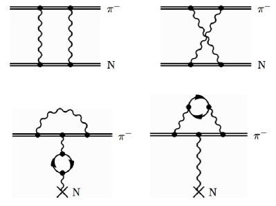
Figure 1: Diagrams relative to the unevaluated QED contributions: second order recoil correction (top), and vacuum polarization and self-energy mixed diagrams (bottom). Their effects are estimated using the available formulas for spin-$\frac{1}{2}$ particles.

The calculations presented here do not take into account second order recoil effects (Fig. 1 top), or higher QED corrections as vacuum polarization and self-energy mixed diagrams (Fig. 1 botton). The contribution from these terms has been estimated using the formula for a spin-$\frac{1}{2}$ particle with a mass equal to the pion’s. For the $5\to 4$ pionic nitrogen transitions, vacuum polarization and self-energy mixed diagrams contribute in the order of 1 meV for the diagram with the vacuum polarization loop in the nuclear photon line Pachucki (1996) (Fig. 1 bottom-left), and 0.0006 meV for the diagram with the vacuum polarization loop inside the self-energy loop Eides et al. (2001) (Fig. 1 bottom-right). The second order recoil contributions are in the order of 0.04 meV Sapirstein and Yennie (1990) (Fig. 1 top). The largest contribution comes from the unevaluated diagram with the vacuum polarization loop in the nuclear photon line Pachucki (1996).

Assuming a statistical population distribution of the HFS sublevels, we can use Eq. (31) to calculate the mean value of the transitions using the results in Table 2. Comparing this calculation with the one without the HFS, we obtain a value for the HFS shift. For transitions $5g\to 4f$ and $5f\to 4d$ we obtain shifts of 0.8 and 2.2 meV, respectively. These values correspond to a correction to the pion mass between 0.2 and 0.6 ppm.

Table 3: Energy (in eV) contribution for the selected levels in kaonic nitrogen. The first error takes into account neglected next order QED corrections. The second is due to the accuracy of the kaon mass ($\pm 32$ ppm).

	8k-7i	8i-7h
Coulomb	2968.4565	2968.5237
Finite size	0.0000	0.0000
Self Energy	0.0000	0.0000
Vac. Pol. (Uehling)	1.1678	1.8769
Vac. Pol. Wichman-Kroll	-0.0007	-0.0008
Vac. Pol. Loop after Loop	0.0007	0.0016
Vac. Pol. Källén-Sabry	0.0111	0.0152
Relativistic Recoil	0.0025	0.0025
HFS Shift	-0.0006	-0.0008
Total	2969.6374	2970.4182
Error	0.0005	0.0005
Error due to the kaon mass	0.096	0.096

Table 4: Hyperfine transition energies and transition rate in kaonic nitrogen.

Transition	F-F’	Trans. rate (s-1)	Trans. E (eV)	Shift (eV)
$8i\to 7h$	7-6	$1.19\times 10^{13}$	2970.4169	-0.00216
	6-5	$1.00\times 10^{13}$	2970.4196	0.00050
	6-6	$0.98\times 10^{13}$	2970.4145	-0.00453
	5-4	$0.84\times 10^{13}$	2970.4217	0.00265
	5-5	$0.03\times 10^{13}$	2970.4175	-0.00154
	5-6	$0.00\times 10^{13}$	2970.4125	-0.00656
$8k\to 7i$	8-7	$1.54\times 10^{13}$	2969.6365	-0.00149
	7-6	$1.33\times 10^{13}$	2969.6383	0.00029
	7-7	$1.31\times 10^{13}$	2969.6347	-0.00326
	6-5	$1.15\times 10^{13}$	2969.6398	0.00178
	6-6	$0.03\times 10^{13}$	2969.6367	-0.00126
	6-7	$0.00\times 10^{13}$	2969.6332	-0.00480

The transition energies for the $8\to 7$ transitions in kaonic nitrogen are presented in Tables 3 and 4. As for the pionic nitrogen, the error contribution due to the QED correction not considered is dominated by the unevaluated diagram with the vacuum polarization loop in the nuclear photon line Pachucki (1996), the associated correction is estimated in the order of 0.5 meV. For $8k\to 7i$ and $8i\to 7h$ transitions we have a HFS shift of 0.6 and 0.8 meV, respectively, which correspond to a correction of the kaon mass between 0.2 and 0.3 ppm.

As a general note, we remark that if we assume a statistical distribution of the initial state sublevels populations, transitions $nl\to n^{\prime}s$ with a $s$ orbital as final state have an average HFS shift equal to zero due to an exact cancellation between the weighted excited sublevels energy shifts as seen from Eq. (31).

IV.2 General behavior of the hyperfine structure correction over Z

For the non-relativistic case, the HFS splitting normalized to the binding energy and to the nuclear magnetic moment, depends linearly on $Z\alpha$. Any deviation from this linear dependence in the Klein-Gordon HFS can be attributed only to relativistic effects.

To study the behavior of the normalized HFS splitting $(E^{9p}_{F=3/2}-E^{9p}_{F=3/2})/({\mathcal{E}}_{0}\mu_{I})$ for the relativistic case, we calculated the HFS for a selected choice of pionic atoms with a stable nucleus of spin 1/2. The orbital $9p$ has been chosen to minimize the effect of the finite nuclear size and strong interaction shifts, particularly for high values of $Z$. The results are summarized in Table 5. For these calculations we used the nuclear mass values from Ref. Audi et al. (2003), the nuclear radii from Refs. Mohr and Taylor (2005); Angeli (2004) and the nuclear magnetic moments from Ref. Raghavan (1989).

For higher $Z$ values a non-linear dependence on $Z\alpha$ appears as we can see in Fig. 2. This non-linearity originates in the two different parts of Eq. (30): the non-trivial dependency on ${\mathcal{E}}_{0}$ in the denominator and the expectation value $\langle nl|r^{-3}|nl\rangle$.

Table 5: HFS separation of the F=1/2 and F=3/2 levels for the $9p$ orbital for pionic atoms with spin $\frac{1}{2}$ nucleus.

Element	Z	$9p$ energy (eV)	HFS splitting (eV)
$\mathrm{H}$	1	-39.93816	0.0001
$\mathrm{{}^{3}He}$	2	-174.8370	-0.0009
$\mathrm{{}^{13}C}$	6	-1633.402	0.0060
$\mathrm{{}^{15}N}$	7	-2226.813	-0.0039
$\mathrm{{}^{19}F}$	9	-3689.435	0.0767
$\mathrm{{}^{31}P}$	15	-10286.63	0.1544
$\mathrm{{}^{57}Fe}$	26	-31023.63	0.0643
$\mathrm{{}^{77}Se}$	34	-53146.21	0.8293
$\mathrm{{}^{89}Y}$	39	-69987.00	-0.3143
$\mathrm{{}^{107}Ag}$	47	-101681.2	-0.4266
$\mathrm{{}^{129}Xe}$	54	-134178.0	-4.1295
$\mathrm{{}^{183}W}$	74	-250634.4	1.2629
$\mathrm{{}^{202}Pb}$	82	-306731.6	7.8662

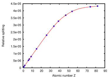
Figure 2: Value of relative splitting $(E^{9p}_{F=3/2}-E^{9p}_{F=3/2})/({\mathcal{E}}_{0}\mu_{I})$ for pionic atoms with different values of $Z$. Nuclear masses, radii and magnetic moments values have been obtained from Refs. Audi et al. (2003); Angeli (2004); Mohr and Taylor (2005); Raghavan (1989).

V Conclusions

We presented a relativistic calculation of the hyperfine structure in pionic and kaonic atoms. The precise evaluation of the specific case of pionic and kaonic nitrogen is particularly important for the new measurement of the pion and kaon mass. The small error on the theoretical predictions, of the order of 1 meV for the $5\to 4$ transition, corresponds to a systematic error of $\gtrsim 0.2$ ppm for the pion mass evaluation, considerably smaller than the error of previous theoretical predictions Schröder et al. (2001).

The formalism presented in this article can be applied for other effect as the quadrupole nuclear moment which can not be negligible for mesonic atoms with high $Z$. In this case, HFS due to the quadrupole moment can be predicted using the next multipole in the development of the electric potential of the nucleus to evaluate the correspondent perturbation operator. This application is particularly important for the calculation of the atomic levels in heavy pionic ions, where relativistic and nucleus deformation effects can be taken into account at the same time.

References

- Gotta (2004) D. Gotta, Progress in Particle and Nuclear Physics 52, 133 (2004).
- Beer et al. (2002) G. Beer, A. M. Bragadireanu, W. Breunlich, M. Cargnelli, C. Curceanu (Petrascu), J.-P. Egger, H. Fuhrmann, C. Guaraldo, M. Giersch, M. Iliescu, et al., Phys. Lett. B 535, 52 (2002).
- Gasser and Leutwyler (1984) J. Gasser and H. Leutwyler, Appl. Phys. 158, 142 (1984).
- Lyubovitskij and Rusetsky (2000) V. E. Lyubovitskij and A. Rusetsky, Phys. Lett. B 494, 9 (2000).
- Gasser et al. (2002) J. Gasser, M. A. Ivanov, E. Lipartia, M. Mojzis, and A. Rusetsky, Eur. Phys. J. C 26, 13 (2002), eprint hep-ph/0206068.
- Pionic Hydrogen Collaboration (1998) Pionic Hydrogen Collaboration, PSI experiment proposal R-98.01 (1998), URL http://pihydrogen.web.psi.ch.
- Anagnostopoulos et al. (2003a) D. F. Anagnostopoulos, M. Cargnelli, H. Fuhrmann, M. Giersch, D. Gotta, A. Gruber, M. Hennebach, A. Hirtl, P. Indelicato, Y. W. Liu, et al., Nucl. Phys. A 721, 849c (2003a).
- Beer et al. (2005) G. Beer, A. M. Bragadireanu, M. Cargnelli, C. Curceanu-Petrascu, J.-P. Egger, H. Fuhrmann, C. Guaraldo, M. Iliescu, T. Ishiwatari, K. Itahashi, et al. (DEAR Collaboration), Phys. Rev. Lett. 94, 212302 (pages 4) (2005).
- Anagnostopoulos et al. (2003b) D. F. Anagnostopoulos, D. Gotta, P. Indelicato, and L. M. Simons, Phys. Rev. Lett. 91, 240801 (2003b).
- Lenz et al. (1998) S. Lenz, G. Borchert, H. Gorke, D. Gotta, T. Siems, D. F. Anagnostopoulos, M. Augsburger, D. Chatellard, J. P. Egger, D. Belmiloud, et al., Phys. Lett. B 416, 50 (1998).
- Pion Mass Collaboration (1997) Pion Mass Collaboration, PSI experiment proposal R-97.02 (1997).
- Nelms et al. (2002) N. Nelms, D. F. Anagnostopoulos, M. Augsburger, G. Borchert, D. Chatellard, M. Daum, J. P. Egger, D. Gotta, P. Hauser, P. Indelicato, et al., Nucl. Instrum. Meth. A 477, 461 (2002).
- Trassinelli (2005) M. Trassinelli, Ph.D. thesis, Université Pierre et Marie Curie, Paris, France (2005), URL http://tel.ccsd.cnrs.fr/tel-00067768.
- Ebersold et al. (1978) P. Ebersold, B. Aas, W. Dey, R. Eichler, H. J. Leisi, W. W. Sapp, and F. Scheck, Nucl. Phys. A 296, 493 (1978).
- Koch and Scheck (1980) J. Koch and F. Scheck, Nucl. Phys. A 340, 221 (1980).
- Scheck (1983) F. Scheck, Leptons, Hadrons, and Nuclei (Elsevier, North-Holland, 1983), 1st ed.
- Austen and de Swart (1983) G. Austen and J. de Swart, Phys. Rev. Lett. 50, 2039 (1983).
- Owen (1994) D. A. Owen, Found. Phys. 24, 273 (1994).
- Trassinelli et al. (2006) M. Trassinelli, D. F. Anagnostopoulos, G. Borchert, A., Dax, J. P. Egger, D. Gotta, M. Hennebach, P. Indelicato, Y.-W. Liu, et al. (2006), in preparation.
- Bjorken and Drell (1964) J. Bjorken and S. Drell, Relativistic Quantum Mechanics (McGraw-Hill Book Company, San Francisco, 1964), 1st ed.
- Decker et al. (1987) R. Decker, H. Pilkuhn, and A. Schlageter, Z. f. Physik 6, 1 (1987).
- Lee et al. (2006) R. N. Lee, A. I. Milstein, and S. G. Karshenboim, Phys. Rev. A 73, 012505 (pages 4) (2006).
- Friar (1980) J. L. Friar, Z. f. Physik 297, 147 (1980).
- Leon and Seki (1981) M. Leon and R. Seki, Nucl. Phys. A 352, 477 (1981).
- Schwartz (1955) C. Schwartz, Phys. Rev. 97, 380 (1955).
- Lindgren and Rosén (1974) I. Lindgren and A. Rosén, Case Studies in Atomic Physics 4, 93 (1974).
- Cheng and Childs (1985) K. Cheng and W. Childs, Phys. Rev. A 31, 2775 (1985).
- Bohr and Weisskopf (1950) A. Bohr and V. F. Weisskopf, Phys. Rev. 77, 94 (1950).
- Edmonds (1974) A. R. Edmonds, Angular Momentum in Quantum Mechanics (Princeton University Press, 1974), 3rd ed.
- Lindgren and Morrison (1982) I. Lindgren and J. Morrison, Atomic Many-Body Theory, Atoms and Plasmas (Springer, Berlin, 1982), 2nd ed.
- Varshalovich et al. (1988) D. A. Varshalovich, A. N. Moskalev, and V. K. Khersonskii, Quantum Theory of Angular Momentum (World Scientific, Singapore, 1988), 1st ed.
- Bethe and Salpeter (1957) H. B. Bethe and E. E. Salpeter, Quantum Mechanics of One- and Two-Electron Atoms (Springer-Verlag, 1957), 1st ed.
- Desclaux (1975) J. P. Desclaux, Comp. Phys. Comm. 9, 31 (1975).
- Desclaux (1993) J. P. Desclaux, in Methods and Techniques in Computational Chemistry, edited by E. Clementi (STEF, Cagliary, 1993), vol. A: Small Systems of METTEC, p. 253, URL hhtp://dirac.spectro.jussieu.fr/mcdf.
- Boucard and Indelicato (2000) S. Boucard and P. Indelicato, Eur. Phys. J. D 8, 59 (2000).
- Desclaux et al. (2003) J. Desclaux, J. Dolbeault, M. Esteban, P. Indelicato, and E. Séré, in Computational Chemistry, edited by P. Ciarlet (Elsevier, 2003), vol. X, p. 1032.
- Santos et al. (2005) J. P. Santos, F. Parente, S. Boucard, P. Indelicato, and J. P. Desclaux, Phys. Rev. A 71, 032501 (pages 8) (2005).
- Béretetski et al. (1989) V. Béretetski, E. Lifchitz, and L. Pitayevsky, Électrodynamique Quantique, Physique Theorique (Éditions MIR, Moscou, 1989), 2nd ed.
- Audi et al. (2003) G. Audi, A. Wapstra, and C. Thibault, Nucl. Phys. A 729, 337 (2003).
- Boucard (2000) S. Boucard, Ph.D. thesis, Université Pierre et Marie Curie, Paris, France (2000), URL http://tel.ccsd.cnrs.fr/tel-00067768.
- Eidelman et al. (2004) S. Eidelman, K. Hayes, K. Olive, M. Aguilar-Benitez, C. Amsler, D. Asner, K. Babu, R. Barnett, J. Beringer, P. Burchat, et al., Phys. Lett. B 592, 1+ (2004), URL http://pdg.lbl.gov.
- Angeli (2004) I. Angeli, At. Data Nucl. Data Tables 87, 185 (2004).
- Fullerton and Rinker (1976) L. W. Fullerton and G. A. Rinker, Phys. Rev. A 13, 1283 (1976).
- Huang (1976) K. N. Huang, Phys. Rev. A 14, 1311 (1976).
- Jeckelmann (1985) B. Jeckelmann, Tech. Rep., ETHZ-IMP (1985), lB-85-03.
- Barker and Glover (1955) W. A. Barker and F. N. Glover, Phys. Rev. 99, 317 (1955).
- Pachucki (1996) K. Pachucki, Phys. Rev. A 53, 2092 (1996).
- Eides et al. (2001) M. I. Eides, H. Grotch, and V. A. Shelyuto, Phys. Rep. 342, 63 (2001).
- Sapirstein and Yennie (1990) J. R. Sapirstein and D. R. Yennie, in Quantum Electrodynamis, edited by T. Kinoshita (World Scientific, 1990), vol. 7 of Directions in High Energy Physics, p. 560.
- Mohr and Taylor (2005) P. J. Mohr and B. N. Taylor, Rev. Mod. Phys. 77, 1 (2005).
- Raghavan (1989) P. Raghavan, At. Data Nucl. Data Tables 42, 189 (1989).
- Schröder et al. (2001) H. C. Schröder, A. Badertscher, P. F. A. Goudsmit, M. Janousch, H. Leisi, E. Matsinos, D. Sigg, Z. G. Zhao, D. Chatellard, J.-P. Egger, et al., Eur. Phys. J. C 21, 473 (2001).