Multiple time scales and the empirical models for stochastic volatility

Abstract

The most common stochastic volatility models such as the Ornstein-Uhlenbeck (OU), the Heston, the exponential OU (ExpOU) and Hull-White models define volatility as a Markovian process. In this work we check of the applicability of the Markovian approximation at separate times scales and will try to answer the question which of the stochastic volatility models indicated above is the most realistic. To this end we consider the volatility at both short (a few days) and long (a few months)time scales as a Markovian process and estimate for it the coefficients of the Kramers-Moyal expansion using the data for Dow-Jones Index. It has been found that the empirical data allow to take only the first two coefficients of expansion to be non zero that define form of the volatility stochastic differential equation of Itô. It proved to be that for the long time scale the empirical data support the ExpOU model. At the short time scale the empirical model coincides with ExpOU model for the small volatility quantities only.
PACS: 89.65.Gh; 02.50.Ey; 02.50.Ga; 02.50.Cw
Keywords: Stochastic volatility models; Volatility autocorrelation; Leverage; Fokker-Plank equation

1. Introduction

The stochastic volatility (SV) models with continuous time have been introduced into literature in late of 80-s of the last century [1, 2, 3, 4]. According to these models the market dynamics is the two-dimensional stochastic process in which the asset price $S_{t}$ obeys the stochastic differential equation in the Itô form ( the index $t$ is omitted for simplicity)

$$dS=\mu Sdt+\sigma SdW_{1}(t),$$ (1)

where the parameter $\mu$ is the drift coefficient, $W_{1}(t)$ is a standard Wiener process and $\sigma_{t}$ is the volatility considered as a stochastic variable.

The empirical analysis have established two important stylized facts concerning with the volatility. Firstly, this process has a long memory emerging, in particular, in that the autocorrelation function absolute returns decay very slowly with time. One can separate, at least, two characteristic time scales in the behavior of the autocorrelation function. At the initial stage there is a fast decay on the short time scale of the order of few days followed by the slow decay during a few months, defining the long time scale. Secondly, there is the negative correlation between past returns change and future volatility (so-called ”leverage” effect).

At the present different SV models are discussed in literature. To a certain extent these models are based either on the model of the geometrical Brownian motion or originate from Ornstein-Uhlenbeck (OU) process. It is assumed that volatility is a function $\sigma=g(Y)$ of a stochastic process $Y_{t}$ and that the dynamic equation for $Y_{t}$ can be represented as a stochastic differential equation in Itô form

$$dY=\alpha(m-Y)dt+f(Y)dW_{2}(t),$$ (2)

$$\sigma=g(Y)\,.$$

Eq.(2) defines the so-called class of mean-reverting processes in which $Y_{t}$ goes to mean value $m$ at $t\to\infty$ with the velocity $\alpha$.The quantity $1/\alpha$ is the time of relaxation of $\sigma$ to its equilibrium value approximately equal to $g(m)$ and actually represents the characteristic time scale of the process. The Wiener process $W_{2}(t)$ in general is correlated with the process $W_{1}(t)$.

Depending on $g$ and $f$ one can distinguish basically four frequently used SV models.
1) The Ornstein-Uhlenbeck (OU) model [1, 2] with $\sigma=Y$ and $f(y)=k$, where $k$ is a positive constant and

$$d\sigma=\sigma(m-Y)dt+kdW_{2}(t)$$ (3)

2) The exponential Ornstein-Uhlenbeck (ExpOU) model [1] with $\sigma=e^{y}$ and $f(y)=k>0$, where it is assumed that $Y=\ln\sigma$ follows to the OU process and variable $\sigma$, as it is easy to show in this case, satisfies the equation

$$d\sigma=\sigma\left[\frac{k^{2}}{2}-\alpha(\ln\sigma-m)\right]dt+k\sigma dW_{2}(t)$$ (4)

3)The Heston model [3] where $\sigma=\sqrt{y}$ and $f(y)=k\sqrt{y}$, $(k>0)$. In this model it is assumed that the volatility is the OU process of the form (3).

4) The Hull-White model [4]with $\sigma=\sqrt{y}$, $f(y)=ky$, $(k>0))$ and

$$d\sigma=\frac{1}{2\sigma}\left[\alpha(m-\sigma^{2})-\frac{k^{2}\sigma^{2}}{4}\right]dt+\frac{k\sigma}{2}dW_{2}(t)$$ (5)

Originally the parameters of the models 1) - 4) were being estimated by a fitting to the empirical data from options pricing. Lately the question about the applicability of one or the other stochastic volatility model for describing a time evolution of stock prices, market indices or exchange rates is actively discussed in the physical literature. The fundamental problem is finding the most realistic model and estimating its parameters.

One of the approaches is that parameters of a model are estimated by fitting the theoretical probability distribution functions (PDF) of returns to the empirical curves. So the studies carried out in works [5, 6, 7, 8] have showed that the Heston model well enough reproduce the empirical distributions for Dow - Jones Index and a number of stocks. On the other hand, in the case of the high-frequency data, the Heston model, as well as Hull-White model, applied to German DAX Index give the return distributions not conforming to tails of the empirical curves [9](see also [10]).

The alternative approach is to estimate the parameters of the above models in such a way as to reproduce other the market stylized facts.In particular, in works [11, 12, 13, 14] the parameters of the OU, Heston and ExpOU models have been estimated by comparison of the theoretical predictions to the observed leverage effect. It has been showed that these models qualitatively reproduce the observed effect as a result of the choice of the parameters, however, the empirical data do not allow to assert the most appropriate model. As regards the autocorrelation function, in contrast with other models, ExpOU qualitatively reproduces the behavior of the empirical curve at medium and long times by fitting the parameters. On the other hand in order to take into account the occurrence of two time scale in the work [15] (see also [16]) a three dimensional diffusion model, assuming that the mean reverting level $m$ is random, has been introduced.

Thus by fitting the parameters above SV models sometimes can reproduce well enough the probability densities of the returns or describe specific observed authoritativeness (the leverage effect, behavior of autocorrelation function). However the question of choice of most realistic stochastic volatility model still remains open.

Models 1) - 4) determinate the volatility as a Markovian process. This follows from the well-known fact that solutions of a SDE of Itô have the Markovian properties [17]. At the same time the empirical volatility autocorrelation function, decaying very slowly with time, shows , in general, the non-Markovian behavior. Furthermore as it has been noted above the autocorrelation function has at least two characteristic time scales. In this connection it is worth noting that the empirical analysis reveals the presence of a well-separated time scales in the dynamics of the volatility itself.

So, LeBaron in [18] has showed that the SV model, where the volatility behavior at short ($\sim 1$ day), medium ($\sim 5$ weeks) and long ($\sim 5$ years) time scales is defined by three different stochastic processes, reproduces power law in the asymptotic of log returns of the Dow-Jones Index and long memory in the volatility fluctuations.

In the work of J.-P. Fouque at al [19] (see also [20]) volatility dynamics both at short (a few days) and long (few a months) time scales was considered within the scope of the ExpOU model but with different relaxation times for each scale. For S&P 500 high-frequency data the short time scale has been found of order $\alpha^{-1}\sim 1.5$ days.

In this work we want to check the application of the above SV models separately both at short and long the time scales. If at the specific time scale the Markovian approximation is applicable, then the coefficients of the SDE of Itô written as

$$d\sigma=D_{1}(\sigma)dt+\sqrt{2D_{2}(\sigma)}dW_{2}(t)$$ (6)

can be obtained from the known expression of the theory of Markovian processes [21]

$$D_{k}(x)=\mathop{\lim}\limits_{\tau\to 0}\frac{1}{\tau}\frac{1}{k!}\int\ {dx^{\prime}(x^{\prime}-x)^{k}p(x^{\prime},t+\tau|x,t)},$$ (7)

where $p(x^{\prime},t^{\prime}|x,t)$ is the conditional PDF and $D_{k}$ are the coefficients of the Kramers-Moyal expansion. Such approach has recently been used in [22, 23] and allowed directly from the data to estimate the coefficients of SDE of Itô for returns handling high-frequency dynamics of DEM/USD exchange rates. Here this method is applied to both high-frequency and low-frequency data. The SDEs of the form (6) obtained for this two data sets have to define the volatility behavior both at short and long time scales. In the end this gives an opportunity to make a comparison with the known SV models and, to a certain extent, to answer the question of how consistent one or the other model is with the empirical data.

The paper is organized as follows. Section 2 is devoted to describing the method of determination of the volatility time series. In Section 3 the coefficients of the Kramers-Moyal expansion have been obtained for different time scales. In Section 4. the numerical solution of the Fokker-Plank equation for conditional PDF is given and the convergence of the solutions to the stationary distributions is considered for both time scales. In section 5 on the basis of the obtained SDE for volatility the simulation of the return series is carried out and its properties are studied. The analysis of the results is given in conclusion.

2. The estimation of volatility and data sets

Unlike prices changes the volatility is not directly observed. At the present there are a different methods of its estimation (for example, see [14, 24]). Most frequently the volatility at the moment of time $t$ is estimated as the standard deviation

$$\sigma_{t}^{2}=\frac{1}{T}\sum\limits_{t^{\prime}=t}^{t+T}(r_{t^{\prime}}-<{r_{t}}>)^{2},$$ (8)

$$<r_{t}>=\frac{1}{N}\sum\limits_{t^{\prime}=t}^{t+T}r_{t^{\prime}},$$

where $r_{t}=\ln S_{t}/S_{t-\Delta}$ are log-returns and an average is carried out over time window $T=(N-1)\Delta$ with an integer $N$.

The two different data sets have been used for the empirical analysis: the high-frequently data set (HFD) for the Dow-Jones Index (data sampled at 5 min intervals from Feb. 16, 2001 to Feb. 26, 2005) and low-frequently data (LFD) (with daily data for the Dow-Jones Index from Jan. 2, 1990 to Feb. 25, 2005). One has respectively $\Delta=5$ min, T=2 hours for HFD and $\Delta=1$ day, T=1 month (21 days) for LFD. The non-overlapping intervals of averaging T have been used for calculation of the volatility given Eq.(8) and respectively the sampling time interval for the volatility data equals T.

The obtained empirical values $\sigma_{t}$ have been used for the construction of the stationary distributions of the volatility and the conditionals PDFs. In doing so it has been assumed that the volatility is a stationary process [14].

3. The estimation of the Kramers-Moyal coefficients

According to what was said in the introduction we shall consider the volatility on the above indicated time scales in the Markovian approximation. In this case, as it is known, the conditional probability density obeys a master equation in the form of a Kramers-Moyal expansion [21].

$$\frac{\partial}{\partial t}p(\sigma,t|\sigma_{0},t_{0})=\sum\limits_{k=1}^{\infty}{\left({-\frac{\partial}{\partial\sigma}}\right)^{k}D_{k}(\sigma)p(\sigma,t|\sigma_{0},t_{0})}$$ (9)

where the coefficients $D_{k}$ are defined as

$$D_{k}(\sigma)=\mathop{\lim}\limits_{\Delta t\to 0}\frac{M_{k}(\sigma,\Delta t)}{\Delta t}$$ (10)

and moments $M_{k}$ are

$$M_{k}(\sigma,\Delta t)=\frac{1}{k!}\int\ {(\tilde{\sigma}-\sigma)^{k}p(\tilde{\sigma},t+\Delta t|\sigma,t)d\tilde{\sigma}}$$ (11)

In this section we shall calculate the coefficients $D_{1}$ and $D_{2}$ of the expansion (9) and show that with enough accuracy the data set allows to take $D_{4}$ to be zero. According to Pawla’s theorem [21] at $D_{4}=0$ all coefficients $D_{k}$ with $k\geq 3$ vanish and the equation (9) reduces to a Fokker-Plank equation. In this case it is coefficients $D_{1}$ and $D_{2}$ that define the form of SDE for volatility of the form (6).

For the calculation of the moments $M_{k}$ the conditional densities $p(\tilde{\sigma},t+\Delta t|\sigma,t)$ (see Fig.4) have been determinated from the empirical data and the numerical integration in (11) has been performed. Further the approximation of the limiting passage $\Delta t\rightarrow 0$ in (10) has been employed and coefficients $D_{1}$ and $D_{2}$ have been obtained.

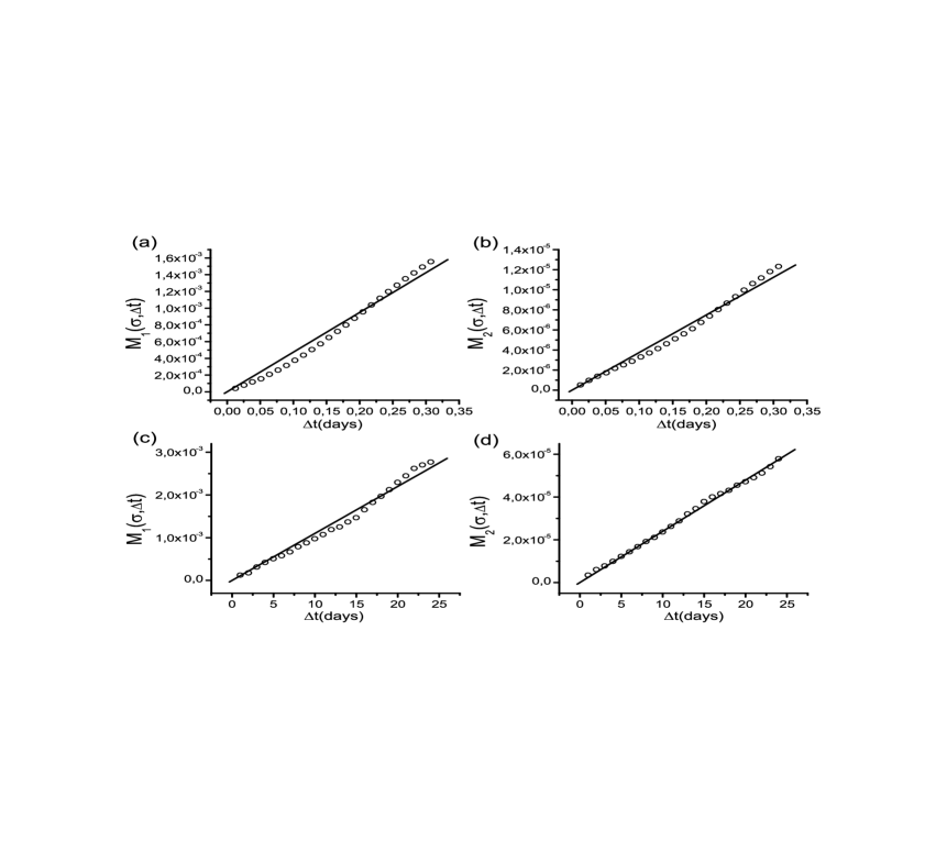
Figure 1: The typical dependence of $M_{1,2}(\sigma,\Delta t)$ on $\Delta t$ at small $\sigma$ (solid line). Circles correspond to the quantities obtained from Eq.(11). Figs.1a,1b correspond to HFD set at $\sigma=0.032$; Figs. 1c, 1d correspond to LFD set at $\sigma=0.02$.

Fig.1 shows some typical dependence of the moments $M_{1,2}$ of $\Delta t$. In order to obtain the moments $M_{1,2}(\sigma,\Delta t)$ for the case of the small $\Delta t$, the volatility given Eq.(8) has been calculated using the overlapping intervals T. At the small $\sigma$ the moments $M_{1,2}$ are well enough described by the linear dependence on $\Delta t$. Therefore the limit in (10) has been approximated as follows

$$\mathop{\lim}\limits_{\Delta t\to 0}\frac{M_{k}(\sigma,\Delta t)}{\Delta t}\approx\frac{M_{k}(\sigma,\Delta t)}{\Delta t}$$ (12)

at $\Delta t=T$. At large $\sigma$ values of moments fluctuate drastically because of the decrease of the statistical data. Nevertheless here too limit (10) has been approximated by relationship (12) at $\Delta t=T$.

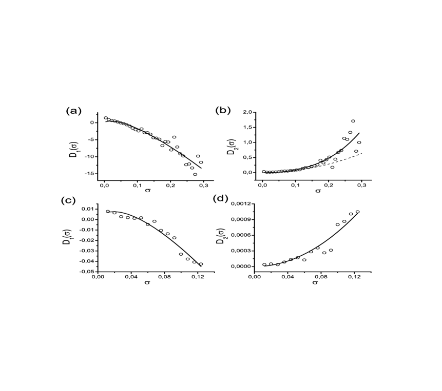
Figure 2: The coefficients $D_{1,2}(\sigma,t)$ obtained from the empirical data using Eqs. (11) and (12) (circles). The solid line is the approximation by the smooth curve. Figs.2a and 2b correspond to HFD set; Figs.2c and 2d correspond to LFD set. The dashed line in Fig. 2b shows the square dependence of $D_{2}$ on $\sigma$.

The results of the calculation of the coefficients $D_{1,2}(\sigma)$ given by Eqs.(10-11) are shown in Fig.2. It has turned out that for both data sets $D_{1}(\sigma)$ can be approximated well enough by the function that coincides in form with the drift coefficient of the ExpOU model (4) (Fig.2a; 2c). For approximation of the coefficient $D_{2}(\sigma)$ for LFD the square dependence on $\sigma$ has been used (Fig. 2d). For HFD for the small $\sigma$, $D_{2}(\sigma)$ can also be approximated by the square dependence on $\sigma$, however, for large $\sigma$ it increases faster then the square function. Therefor for approximation $D_{2}(\sigma)$ for all $\sigma$ the function has been used

$$D_{2}(\sigma)=b_{1}\sigma^{2}\exp(b_{2}\sigma).$$ (13)

In the result of the fitting we have obtained:

for HFD

$$D_{1}^{(H)}(\sigma)=-\sigma(a_{1}-a_{2}\ln(\sigma/\sigma_{0}))$$ (14)

$$D_{2}^{(H)}(\sigma)=b_{1}\sigma^{2}\exp(b_{2}\sigma)$$ (15)

where $a_{1}=-0.071\,{\rm(month)}^{-1}$; $a_{2}=26.5\,{\rm(month)}^{-1}$; $b_{1}=7.08\,{\rm(month)}^{-1}$; $b_{2}=2.65\,{\rm(month)}^{1/2}$; for LFD

$$D_{1}^{(L)}(\sigma)=-\sigma(a_{1}-a_{2}\ln(\sigma/\sigma_{0}))$$ (16)

$$D_{2}^{(L)}(\sigma)=b_{1}\sigma^{2}$$ (17)

where $a_{1}=4.47\,{\rm(month)}^{-1}$; $a_{2}=0.41\,{\rm(month)}^{-1}$; $b_{1}=0.06\,{\rm(month)}^{-1}$. For both data sets $\sigma_{0}$ is the mean volatility equal to $0.044\,{\rm(month)}^{-1/2}$. Correspondingly, the relaxation times are $1/\alpha^{(H)}=1/a_{2}^{(H)}=0.79$ day and $1/\alpha^{(L)}=1/a_{2}^{(L)}=2.43$ month.

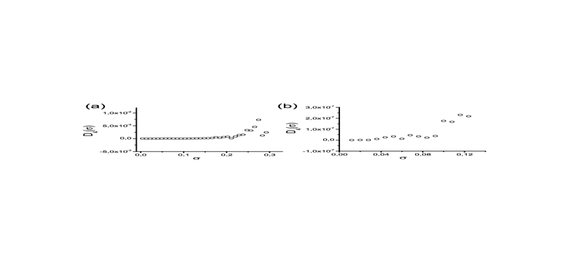
Figure 3: The dependence of the coefficient the $D_{4}$ on $\sigma$ ; (a) - HFD set; (b) - LFD set.

At last, the results of the calculation of the coefficients $D_{4}$ are represented in Fig.3. It is shown that the values of the coefficient $D_{4}$ in fact are equal to zero, the fluctuations do not exceed $10^{-2}$ for HFD and $3\cdot 10^{-7}$ for LFD which is a few orders less than the corresponding values of $D_{1}$ and $D_{2}$.

4. The numerical solution of the Fokker-Plank equation

As it has been noted in the previous section at $D_{4}=0$ the master equation (9) reduces to the Fokker-Plank equation

$$\frac{\partial}{\partial t}p(\sigma,t_{0}|\sigma_{0},t_{0})=\left\{{-\frac{\partial}{\partial\sigma}D_{1}(\sigma)+\frac{\partial^{2}}{\partial\sigma^{2}}D_{2}(\sigma)}\right\}p(\sigma,t_{0}|\sigma_{0},t_{0})$$ (18)

In this section we shall consider on the basis of a numerical solution of Eq.(18) the time evolution of the conditional densities $p(\sigma,t|\sigma_{0},t_{0})$ and show that the stationary solution of this equation is consistent enough with the empirical densities.

Eq.(18) was solved with at boundary conditions at $\sigma=0$ and $\sigma=\infty$

$$p(\sigma,t_{0}|\sigma_{0},t_{0})|_{\sigma=0;+\infty}=0\hskip 28.45274pt(\sigma\geq 0)$$

and the initial condition $p(\sigma,t_{0}|\sigma_{0},t_{0})=\delta(\sigma-\sigma_{0})$ where $\delta(x)$ is $\delta$-function and $\sigma_{0}=0.044$. For the numerical solution of the Fokker-Plank equation (18) the finite-difference method given in [22] has been used.

The conditional densities $p(\sigma,t|\sigma_{0},t_{0})$ for different times $t$ are represented in Fig.4. As it is shown from Fig.4a for high-frequency data the stationary state is reached within $t\simeq 1.5$ days (from this on time the theoretical curves practically coincide). For low-frequency data the stationary state is settling within the time of the order of 5 months (Fig.4c). As it is shown from Fig.4b;4c the theoretical stationary distributions are consistent enough with the empirical volatility densities. To some extent this fact can serve as validation of estimating the coefficients $D_{1,2}$.

5. The simulation of the return series

As it is known [17, 21] the Fokker-Plank equation (18) is equivalent to the SDE of Itô of the form

$$d\sigma=D_{1}(\sigma)dt+\sqrt{2D_{2}(\sigma)}dW_{2}(t)$$ (19)

This equation in combination with Eq.(1) enables to perform the simulation of the prices series that gives an opportunity to obtain a theoretical return PDF.

In order to eliminate the parameter $\mu$ in Eq.(1) let us introduce the new variable $x_{t}=\ln S_{t}/S_{0}-\mu t$, where $S_{0}$ is the initial price. It is easy to obtain that

$$dx_{t}=-\frac{\sigma_{t}^{2}}{2}dt+\sigma_{t}dW_{1}(t).$$ (20)

Using Eqs.(19) and (20) and the explicit form of the coefficients $D_{1}$ and $D_{2}$ for both data sets we have generated the series $x_{t}$. The Wiener processes $W_{1}(t)$ and $W_{2}(t)$ have been assumed to be independent. The found price series have been used for the plotting of the probability density and the autocorrelation function of the absolute log-returns.

Fig.5 represents the plots of PDF of the prices changes $\triangle x=\ln S_{t}/S_{t-\triangle}-\mu\triangle$ obtained from both the generated price series and the empirical data. As it is seen there is a good agreement between the corresponding curves.

The plots of the autocorrelation function of the absolute log-returns $|r_{t}|$ are given in Fig.6. In the case of high-frequency dynamics (Fig.6a) there is a rapid decay of the empirical autocorrelation function at the time of the order of one day followed by a more slow decrease (solid line). The generated curves reproduces this abrupt drop (dashed line) at time of the order of 1.5 days. The same behavior is also exhibited for S&P500 Index [19]. The periodic oscillations of the empirical correlation function arises from a stable increase of the trade activity at both the beginning and the end of day.

In the case of low-frequency dynamics the generated autocorrelation function reproduces the initial drop of the empirical curve at times of the order of two months (Fig.6b).

6. Conclusion

The SV models introduced in [1, 2, 3, 4] define the volatility as a Markovian process. On the other hand the volatility autocorrelation function shows the existence of two or more characteristic times,which, in general, is not typical for the Markovian processes. In recent works [18, 19, 20] the SV models have been considered, describing volatility as a superposition of Markovian processes with different characteristic times. Using these approaches we consider volatility at both short and long time scales in the Markovian approximation. On the basis of the empirical data, employing Eqs.(10) and (11), we estimated the coefficients $D_{1,2}$ of Ito SDE defining the volatility dynamics. It has been shown that for the long time scale the empirical data support the ExpOU model with the characteristic time $\alpha^{-1}=2.43$ months (see Eqs.(16) and (17)). On the short time scale the drift coefficient can also be described within the scope of this model with $\alpha^{-1}=0.79$ days (Eq.(14)). As regards the diffusion coefficient it shows more complicated behavior than a simple square dependence (see Eq.(15)).

On the base of the numerical solution of the Fokker-Plank equation we have considered the time evolution of the conditional PDF $p(\sigma,t|\sigma_{0},t_{0})$. It has been shown that the stationary state settles in accordance with the found relaxation times within time of the order $t\sim 2/\alpha$, where for the long time scale $t_{L}\sim 5$ months and for short time scale $t_{S}\sim 1,5$ days. Very good agreement is found between the calculated stationary densities and the empirical curves (Fig.4). This fact supports the validity of estimating of the coefficients $D_{1,2}$.

On the basis of Eqs (19) and (20) the price series $x_{t}$ has been generated and PDFs of the price changes $\Delta x_{t}=x_{t}-x_{t-\Delta}$ for the different time delays $\Delta$ obtained. In the absence of a correlation between the Wiener processes $W_{1}(t)$ and $W_{2}(t)$ the agreement between the simulated and empirical densities for both time scales is good enough (Fig.5).

On the basis of the generated data the volatility autocorrelation function has been obtained. The empirical autocorrelation function within the interval of a few months shows the existence of at least two characteristic time scales (Fig.6). At the initial stage there is a drop within approximately 0.5 days followed by a slow decay. As it is seen from Fig.6 the generated data at both short (within $\sim 0.5$ days) and long (within $\sim 2$ months) time scale separately describe such behavior.

The obtained results deserve attention especially if one takes into account that the parameters $D_{1,2}$ were not fitted specially to neither the empirical densities nor the behavior of autocorrelation function.

The parameters of the ExpOU model for the Dow-Jones Index were estimated in other works also. In [14] it has been shown that the fitting of the theoretical curve to the empirical volatility autocorrelation function at the interval of a few months gives the estimation of the relaxation time of the order of $35\pm 18$ days. On the upper bound this estimation is close to our results for LFD.

On the other hand the derivation of SDE for the volatility on the basis of the empirical data was also considered in [26]. The equation obtained in this work for the low-frequency dynamics of the Dow-Jones Index is close enough to the Eq.(4) of the ExpOU model. Numerical solution the the Fokker-Plank equation for the conditional PDF has shown that the stationary state settles within 3-4 months, which approximately corresponds to our data.

Thus the results reported in this work show that the employment of the Markovian approximation at the individual time scale in all probability allows to describe at this scale a number of market appropriateness. In particular we have shown that the volatility autocorrelation function and the probability return densities obtained within the scope of this approximation are consistent enough with their empirical analogues separately at both short and long time scales.

Figures

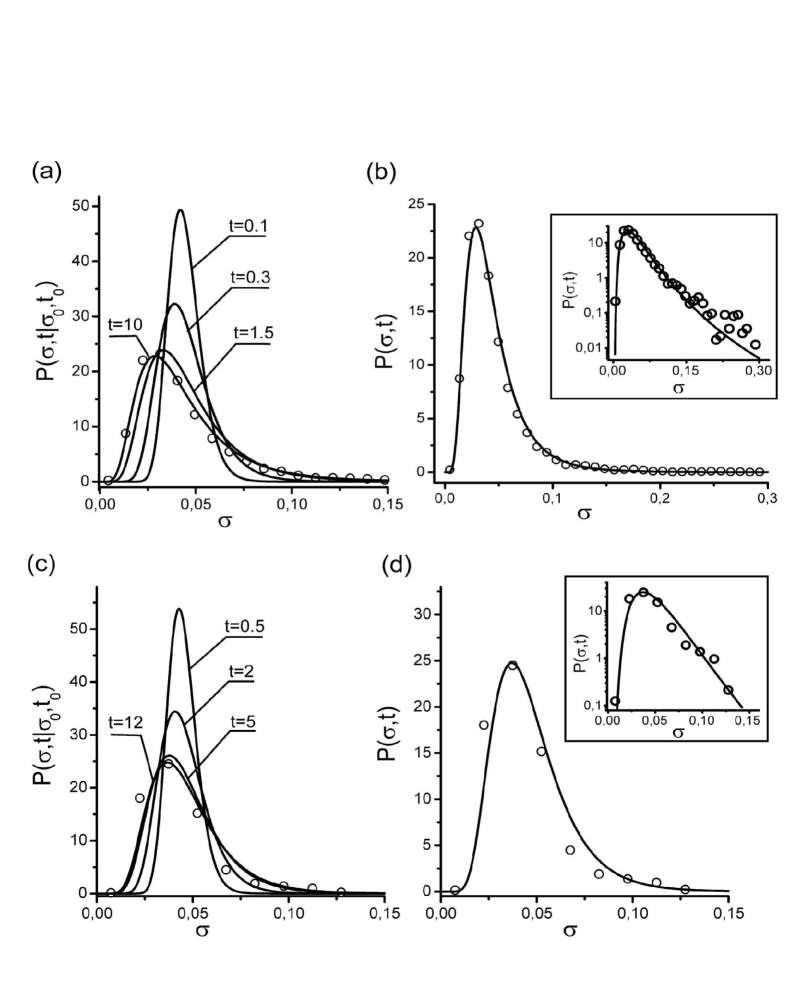
Figure 4: The time evolution of the conditional PDFs $p(\sigma t|\sigma_{0}t_{0})$; (a) - HFD set, $t=0.1;1.5;10;12$ days; (c) - LFD set, $t=0.5;2;5;12$ months; $t_{0}=0$. The solid line in Figs. 4b and 4d correspond the stationary distributions obtained from the Fokker-Plank equation, respectively, for $t=10$ days (HFD) and $t=12$ months (LFD). Circles - the empirical distributions. The inset shows the same curves in the log - log scale.

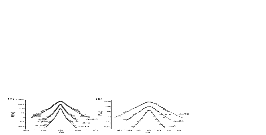
Figure 5: The probability densities of the price changes $\Delta x=\ln S_{t}/S_{t-\Delta}-\mu\Delta$. The solid line have been obtained from the simulated data; circles - the empirical data;(a) - HFD set, $\Delta=0.5;2;6.5$ hours; (b) - LFD set, $\Delta=6;24;72$ days. For convenience of presentation the PDFs are shifted in vertical direction by multiplication by 10.

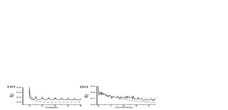
Figure 6: The autocorrelation function of $|r_{t}|$. The dashed line have been obtained from the generated data, the solid line obtained on the basis the empirical data; (a) - HFD set, (b) - LFD set.

References

- [1] L.J. Scott, Option Pricing when the Variance Changes Randomly: Theory, Estimation, and an Application, Fin. Quant. Anal. 22 (1987) 419-438.
- [2] E.M. Stein and J.C. Stein, Stock Price Distributions with Stochastic Volatility: An Analytic Approach, Rev. Financial Studies 4 (1991) 727-752.
- [3] S.L. Heston, A closed-form solution for options with stochastic volatility with applications to bond and currency options, Rev. Financial Studies 6 (1993) 327-343.
- [4] J. Hull, A.J. White, The Pricing of Options on Assets with Stochastic Volatilities, Finance XLII (1987) 281-300.
- [5] A. Dragulescu, V.M. Yakovenko, Probability distribution of returns in the Heston model with stochastic volatility, Quant. Finance 2 (2002) 443-453.
- [6] A. Silva, V. Yakovenko, Comparison between the probability distribution of returns in the Heston model and empirical data for stock indices, Physica A 324 (2003) 303-311.
- [7] A. Silva, R.E. Prange, V.M. Yakovenko, Expotential distribution of financial returns at mesoscopic time lags: a new stylized fact, Physica A 344 (2004) 227-235.
- [8] G.L. Buchbinder, K.M. Chistilin, The description of the Russian stock market within the scope of the Heston model, Math. Model. 17(10) (2005) 31-38 (in Russian).
- [9] R. Remer, R. Mahnke, Application of Heston model and its solution to German DAX data, Physica A 344 (2004) 236-239.
- [10] S. Vicciche, at. al., Volatility in financial markets: stochastic models and empirical results, Physica A 314 (2002) 756-761.
- [11] J. Perello, J. Masoliver, Random diffusion and leverage effect in financial markets, Phys. Rev. E 67 (2003) 037102.
- [12] J. Masoliver, J. Perello, A correlated stochastic volatility model measuring leverage and other stylized facts, Int. J. Theor. Appl. Fin. 5 (2002) 5-41.
- [13] J. Perello, J. Masoliver, N. Anento, A comparison between several correlated stochastic volatility models, Physica A 344 (2004) 134-137.
- [14] J. Perello, J. Masoliver, Multiple time scales and the exponential Ornstein-Uhlenbeck stochastic volatility model, arXiv.org/abs/cond-mat/0501639v1.
- [15] J. Perello, J. Masoliver, J.-P. Bouchaud, Multiple time scales in volatility and leverage correlations: An stochastic volatility model, Appl. Math. Finance 11 (2004) 27-50.
- [16] R. Vicente, at al., Common underlying dynamics in an emerging market: from minutes to months, Physica A 361 (2006) 272.
- [17] C.W. Gardiner, Handbook of stochastic methods for physics, chemistry, and the natural sciences, Springer-Verlag, New York, 1997.
- [18] B. LeBaron, Stochastic volatility as a simple generator of apparent financial power laws and long memory, Quant. Finance 1 (2001) 621-631
- [19] J.-P. Fouque, at al., Short time-scale in S&P 500 volatility, J. Comput. Finance 6 (2003) 1-23.
- [20] J.-P. Fouque, at al., Multiscale stochastic volatility asymptotics, Multiscale. Model. Simul. 2(1) (2003) 22-42.
- [21] H. Risken The Fokker-Planck Equation, Springer, Berlin, 1984.
- [22] R. Friedrich, J. Peinke, Ch. Renner, How to quantify deterministic and random influences on the statistics of the foreign exchange market, Phys. Rev. Lett. 84 (2000) 5224-5227.
- [23] Ch. Renner,J. Peinke, R. Friedrich, Evidence of Markov properties of high frequency exchange rate data, Physica A. 298 (2001) 499-520.
- [24] Yanhui Liu, at al., Statistical properties of the volatility of price fluctuation, Phys. Rev. E 60 (1999) 1390-1400.
- [25] U. Brosa, W. Cassing, Numerical Studies on the Phase-Space Evolution of Relative Motion of Two Heavy Ions, Z. Phys. A 307 (1982) 167-174.
- [26] P. Wilmott, A. Oztukel, Uncertain parameters, an empirical stochastic volatility model and confidance limits, Int. J. Theor. Appl. Fin. 1 (1998) 175-198.