Unified theory for Goos-Hänchen and Imbert-Fedorov effects

Abstract

A unified theory is advanced to describe both the lateral Goos-Hänchen (GH) effect and the transverse Imbert-Fedorov (IF) effect, through representing the vector angular spectrum of a 3-dimensional light beam in terms of a 2-form angular spectrum consisting of its 2 orthogonal polarized components. From this theory, the quantization characteristics of the GH and IF displacements are obtained, and the Artmann formula for the GH displacement is derived. It is found that the eigenstates of the GH displacement are the 2 orthogonal linear polarizations in this 2-form representation, and the eigenstates of the IF displacement are the 2 orthogonal circular polarizations. The theoretical predictions are found to be in agreement with recent experimental results.

I Introduction

In 1947, Goos and Hänchen Goos-H experimentally demonstrated that a totally reflected light beam at a plane dielectric interface is laterally displaced in the incidence plane from the position predicted by geometrical reflection. Artmann Artmann in the next year advanced a formula for this displacement on the basis of a stationary-phase argument. This phenomenon is now referred to as Goos-Hänchen (GH) effect. In 1955, Fedorov Fedorov expected a transverse displacement of a totally reflected beam from the fact that an elliptical polarization of the incident beam entails a non-vanishing transverse energy flux inside the evanescent wave. Imbert Imbert calculated this displacement using an energy flux argument developed by Renard Renard for the GH effect and experimentally measured it. This phenomenon is usually called Imbert-Fedorov (IF) effect. The investigation of the GH effect has been extended to the cases of partial reflection and transmission in transmitting configurations Hsue-T ; Li-W and to other areas of physics, such as acoustics Briers-LS , nonlinear optics Jost-AS , plasma physics Yin-HLFZ , and quantum mechanics Renard ; Ignatovich . And the IF effect has been connected with the angular momentum conservation and the Hall effect of light Onoda-MN ; Bliokh-B . But the comment of Beauregard and Imbert Beauregard-I is still valid up to now that there are, strictly speaking, no completely rigorous calculations of the GH or IF displacement. Though the argument of stationary phase was used to explain Artmann the GH displacement and to calculate the IF displacement Schilling , it was on the basis of the formal properties of the Poynting vector inside the evanescent wave Beauregard-I that the quantization characteristics were acquired for both the GH and IF displacements in total reflection. On the other hand, it has been found that the GH displacement in transmitting configurations has nothing to do with the evanescent wave Li-W .

The purpose of this paper is to advance a unified theory for the GH and IF effects through representing the vector angular spectrum of a 3-dimensional (3D) light beam in terms of a 2-form angular spectrum, consisting of its 2 orthogonal polarizations. From this theory, the quantization characteristics of the GH and IF displacements are obtained, and the Artmann formula Artmann for the GH displacement is derived. The amplitude of the 2-form angular spectrum describes the polarization state of a beam in such a way that the eigenstates of the GH displacement are the 2 orthogonal linear polarizations and the eigenstates of the IF displacement are the 2 orthogonal circular polarizations.

II General theory

Consider a monochromatic 3D light beam in a homogenous and isotropic medium of refractive index $n$ that intersects the plane $x=0$. In order to have a beam representation that can describe the propagation parallel to the $x$-axis, the vector electric field of the beam is expressed in terms of its vector angular spectrum as follows Ghatak-T ,

$$\mathbf{E}(\mathbf{r})=\frac{1}{2\pi}\int^{\infty}_{-\infty}\int^{\infty}_{-\infty}\mathbf{A}(k_{y},k_{z})\exp(i\mathbf{k}\cdot\mathbf{r})dk_{y}dk_{z},$$ (1)

where time dependence $\exp(-i\omega t)$ is assumed and suppressed, $\mathbf{A}=(\begin{array}[]{ccc}A_{x}&A_{y}&A_{z}\end{array})^{T}$ is the vector amplitude of the angular spectrum, $\mathbf{k}=(\begin{array}[]{ccc}k_{x}&k_{y}&k_{z}\end{array})^{T}$ is the wave vector satisfying $k^{2}_{x}+k^{2}_{y}+k^{2}_{z}=k^{2}$, $k=2n\pi/\lambda_{0}$, $\lambda_{0}$ is the vacuum wavelength, superscript $T$ means transpose, and the beam is supposed to be well collimated so that its angular distribution function is sharply peaked around the principal axis $(k_{y0},k_{z0})$ and that the integration limits have been extended to $\pm\infty$ for both variables $k_{y}$ and $k_{z}$ Marcuse . When this beam intersects the plane $x=0$, the electric field distribution on this plane is thus

$$\mathbf{\Psi}(y,z)\equiv\mathbf{E}(\mathbf{r})|_{x=0}=\frac{1}{2\pi}\int\int\mathbf{A}e^{i(k_{y}y+k_{z}z)}dk_{y}dk_{z},$$

hereafter the integration limits will be omitted as such. The position coordinates of the centroid of the beam (1) on the plane $x=0$ are defined by

$$\langle y\rangle=\frac{\int\int\mathbf{\Psi}^{\dagger}y\mathbf{\Psi}dydz}{\int\int\mathbf{\Psi}^{\dagger}\mathbf{\Psi}dydz}=\frac{\int\int\mathbf{A}^{\dagger}i\frac{\partial\mathbf{A}}{\partial k_{y}}dk_{y}dk_{z}}{\int\int\mathbf{A}^{\dagger}\mathbf{A}dk_{y}dk_{z}}$$ (2)

and

$$\langle z\rangle=\frac{\int\int\mathbf{\Psi}^{\dagger}z\mathbf{\Psi}dydz}{\int\int\mathbf{\Psi}^{\dagger}\mathbf{\Psi}dydz}=\frac{\int\int\mathbf{A}^{\dagger}i\frac{\partial\mathbf{A}}{\partial k_{z}}dk_{y}dk_{z}}{\int\int\mathbf{A}^{\dagger}\mathbf{A}dk_{y}dk_{z}},$$ (3)

where $\frac{\partial}{\partial k_{y}}$ means partial derivative with respect to $k_{y}$ with $k_{z}$ fixed, $\frac{\partial}{\partial k_{z}}$ means partial derivative with respect to $k_{z}$ with $k_{y}$ fixed, and superscript $\dagger$ stands for transpose conjugate.

Since the Fresnel formula for the amplitude reflection coefficient at a dielectric interface depends on whether the incident plane wave is in $s$ or $p$ polarization, it is profitable to represent the vector amplitude of the angular spectrum in terms of its $s$ and $p$ polarized components. To this end, let us first consider one plane-wave element of the angular spectrum whose wave vector is $\mathbf{k}^{0}=(\begin{array}[]{ccc}k\cos\theta&k\sin\theta&0\end{array})^{T}$, where $\theta$ is its incidence angle. Its vector amplitude is given by $\mathbf{A}^{0}=\mathbf{A}^{0}_{s}+\mathbf{A}^{0}_{p}\equiv A_{s}\mathbf{s}^{0}+A_{p}\mathbf{p}^{0}$, where $A_{s}$ and $A_{p}$ are the complex amplitudes of $\mathbf{A}^{0}_{s}$ and $\mathbf{A}^{0}_{p}$, respectively, $\mathbf{s}^{0}=(\begin{array}[]{ccc}0&0&1\end{array})^{T}$ is the unit vector of $\mathbf{A}^{0}_{s}$ and is perpendicular to the plane $xoy$, and $\mathbf{p}^{0}=(\begin{array}[]{ccc}-\sin\theta&\cos\theta&0\end{array})^{T}$ is the unit vector of $\mathbf{A}^{0}_{p}$ and is parallel to the plane $xoy$. This means that $\mathbf{A}^{0}$ can be represented as

$$\mathbf{A}^{0}=\left(\begin{array}[]{cc}0&-\sin\theta\\ 0&\cos\theta\\ 1&0\end{array}\right)\tilde{A},$$

where

$$\tilde{A}=\left(\begin{array}[]{c}A_{s}\\ A_{p}\end{array}\right)\equiv A_{s}\tilde{s}+A_{p}\tilde{p}$$ (4)

is what we introduce in this paper and is referred to as the 2-form amplitude of the angular spectrum, $\tilde{s}=\left(\begin{array}[]{c}1\\ 0\end{array}\right)$ represents the normalized state of s polarization, and $\tilde{p}=\left(\begin{array}[]{c}0\\ 1\end{array}\right)$ represents the normalized state of p polarization. $\tilde{s}$ and $\tilde{p}$ form the orthogonal complete set of linear polarizations.

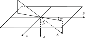
Figure 1: Schematic diagram for the rotation of the vector amplitude $\mathbf{A}$ of an arbitrarily polarized light beam.

After this element is rotated by angle $\varphi$ around the $x$-axis as is displayed in Fig. 1, its wave vector becomes

$$\mathbf{k}=\mathrm{M}(\varphi)\mathbf{k}^{0}=\left(\begin{array}[]{c}k\cos\theta\\ k\sin\theta\cos\varphi\\ k\sin\theta\sin\varphi\end{array}\right),$$

and its vector amplitude becomes

$$\mathbf{A}=\mathrm{M}(\varphi)\mathbf{A}^{0}=A_{s}\mathbf{s}+A_{p}\mathbf{p},$$ (5)

where

$$\mathrm{M}(\varphi)=\left(\begin{array}[]{ccc}1&0&0\\ 0&\cos\varphi&-\sin\varphi\\ 0&\sin\varphi&\cos\varphi\end{array}\right)$$

is the rotation matrix,

$$\mathbf{s}=\mathrm{M}(\varphi)\mathbf{s}^{0}=(\begin{array}[]{ccc}0&-\sin\varphi&\cos\varphi\end{array})^{T}$$

is the unit vector of $\mathbf{A}_{s}=\mathrm{M}(\varphi)\mathbf{A}^{0}_{s}$, and

$$\mathbf{p}=\mathrm{M}(\varphi)\mathbf{p}^{0}=\left(\begin{array}[]{c}-\sin\theta\\ \cos\theta\cos\varphi\\ \cos\theta\sin\varphi\end{array}\right)$$

is the unit vector of $\mathbf{A}_{p}=\mathrm{M}(\varphi)\mathbf{A}^{0}_{p}$. This shows that the vector amplitude (5) can be represented as

$$\mathbf{A}=\left(\begin{array}[]{cc}0&p_{x}\\ s_{y}&p_{y}\\ s_{z}&p_{z}\end{array}\right)\tilde{A}\equiv\mathrm{P}\tilde{A},$$ (6)

where matrix $\mathrm{P}$ represents the projection of 2-form amplitude $\tilde{A}$ onto vector amplitude $\mathbf{A}$ and is thus referred to as projection matrix, and

$$s_{y}=-\sin\varphi=-\frac{k_{z}}{(k^{2}_{y}+k^{2}_{z})^{1/2}}$$

$$s_{z}=\cos\varphi=\frac{k_{y}}{(k^{2}_{y}+k^{2}_{z})^{1/2}}$$

$$p_{x}=-\sin\theta=-\frac{(k^{2}_{y}+k^{2}_{z})^{1/2}}{k}$$

$$p_{y}=\cos\theta\cos\varphi=\frac{k_{x}k_{y}}{k(k^{2}_{y}+k^{2}_{z})^{1/2}}$$

$$p_{z}=\cos\theta\sin\varphi=\frac{k_{x}k_{z}}{k(k^{2}_{y}+k^{2}_{z})^{1/2}}$$

Now we have successfully represented, through the projection matrix, the vector amplitude $\mathbf{A}$ in terms of the 2-form amplitude $\tilde{A}$, that is to say, in terms of the 2 orthogonal linear polarizations $\mathbf{A}_{s}$ and $\mathbf{A}_{p}$. It should be pointed out that in this representation, $\mathbf{s}$ is not necessarily perpendicular to the plane $xoy$, and $\mathbf{p}$ is not necessarily parallel to this plane. Denoting $\mathbf{k}_{r}=k_{r}\mathbf{e}_{r}=k_{y}\mathbf{e}_{y}+k_{z}\mathbf{e}_{z}$, where $k_{y}=k_{r}\cos\varphi$, $k_{z}=k_{r}\sin\varphi$, $\mathbf{e}_{y}$ and $\mathbf{e}_{z}$ are the unit vectors in $y$ and $z$ directions, respectively, and $\mathbf{e}_{r}$ is the unit vector in the radial direction, we find that $\mathbf{s}$ is in fact the unit vector in the azimuthal direction, $\mathbf{s}=\mathbf{e}_{\varphi}$. Furthermore, letting $\mathbf{p}_{r}=p_{y}\mathbf{e}_{y}+p_{z}\mathbf{e}_{z}$, it is apparent that $\mathbf{p}_{r}=\frac{k_{x}}{k}\mathbf{e}_{r}$. In other words, $\mathbf{p}_{r}$ is in the radial direction. The directions of $\mathbf{s}$ and $\mathbf{p}_{r}$ are schematically shown in Fig. 2.

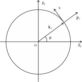
Figure 2: $\mathbf{s}$ and $\mathbf{p}_{r}$ are in the azimuthal and radial directions, respectively.

Unit vectors $\mathbf{s}$ and $\mathbf{p}$ and the wave vector $\mathbf{k}$ are orthogonal to each other and thus satisfy the following relations,

$$\begin{array}[]{r}s^{2}_{y}+s^{2}_{z}=1\\ p^{2}_{x}+p^{2}_{y}+p^{2}_{z}=1\\ s_{y}p_{y}+s_{z}p_{z}=0\\ k_{y}s_{y}+k_{z}s_{z}=0\\ k_{x}p_{x}+k_{y}p_{y}+k_{z}p_{z}=0\end{array}$$ (7)

The first 3 equations guarantee

$$\mathbf{A}^{\dagger}\mathbf{A}=\tilde{A}^{\dagger}\tilde{A}.$$ (8)

From expression (6) for the vector amplitude and with the help of Eq. (7), we obtain

$$\mathbf{A}^{\dagger}\frac{\partial\mathbf{A}}{\partial k_{y}}=\tilde{A}^{\dagger}\frac{\partial\tilde{A}}{\partial k_{y}}-\frac{k_{x}k_{z}}{k(k^{2}_{y}+k^{2}_{z})}(A^{*}_{s}A_{p}-A^{*}_{p}A_{s}),$$ (9)

$$\mathbf{A}^{\dagger}\frac{\partial\mathbf{A}}{\partial k_{z}}=\tilde{A}^{\dagger}\frac{\partial\tilde{A}}{\partial k_{z}}+\frac{k_{x}k_{y}}{k(k^{2}_{y}+k^{2}_{z})}(A^{*}_{s}A_{p}-A^{*}_{p}A_{s}).$$ (10)

Eqs. (2), (3), (8), (9), and (10) are the central results of this paper, from which the GH and IF displacements are derived below.

III Description of incident and reflected beams

Without loss of generality, we consider an arbitrarily polarized incident beam of the following 2-form amplitude,

$$\tilde{A}_{i}=(l_{i1}\tilde{s}+l_{i2}\tilde{p})A\equiv\tilde{L}_{i}A,$$ (11)

where $\tilde{L}_{i}=l_{i1}\tilde{s}+l_{i2}\tilde{p}$ describes the polarization state of the beam and is assumed to satisfy the normalization condition

$$\tilde{L}^{\dagger}_{i}\tilde{L}_{i}=1,$$ (12)

angular distribution function $A(k_{y},k_{z})$ is assumed to be a positively-definite sharply-peaked symmetric function around the principal axis $(k_{y0},k_{z0})=(k\sin\theta_{0},0)$ and satisfy the normalization condition

$$\int\int A^{2}(k_{y},k_{z})dk_{y}dk_{z}=1,$$ (13)

and $\theta_{0}$ stands for the incidence angle of the beam. Eqs. (12) and (13) guarantee the following normalization condition for the 2-form amplitude (11),

$$\int\int\tilde{A}^{\dagger}_{i}\tilde{A}_{i}dk_{y}dk_{z}=1.$$ (14)

One example of such a distribution function that satisfies normalization condition (13) is the following Gaussian function Ghatak-T ; Zhang-L ,

$$A_{G}=\left(\frac{w_{y}w_{z}}{\pi}\right)^{\frac{1}{2}}\exp\left[-\frac{w^{2}_{y}}{2}(k_{y}-k_{y0})^{2}\right]\exp\left(-\frac{w^{2}_{z}}{2}k^{2}_{z}\right),$$ (15)

where $w_{y}=w_{0}/\cos\theta_{0}$, $w_{z}=w_{0}$, $w_{0}$ is half the width of the beam at waist. $\Delta\theta=\frac{1}{kw_{0}}$ is half the divergence angle of the beam.

According to Eq. (6), the vector amplitude of the incident beam is given by $\mathbf{A}_{i}=\mathrm{P}\tilde{A}_{i}$. For a uniformly polarized beam that was obtained from a linearly polarized beam in experiments Pillon-GG ; Pillon-GGLKG ; Pillon-GGLE , the $s$ components of all its plane-wave elements are in the same direction, and the same to the $p$ components. But in our representation advanced here, the $s$ polarizations of different plane-wave elements are generally in different directions; so are the $p$ polarizations. Considering Eqs. (6), (11) and (15) together, one concludes that in order to describe a uniformly polarized beam mentioned above, it is essential that the incidence angle $\theta_{0}$ be much larger than $\Delta\theta$. So we will only consider the case of large $\theta_{0}$ below. Fortunately, this is just what we have in the case of total reflection.

It will be convenient to express $\tilde{L}_{i}$ on the orthogonal complete set of circular polarizations as follows,

$$\tilde{L}_{i}=c_{i1}\tilde{r}+c_{i2}\tilde{l}=\mathrm{U}\tilde{C}_{i},$$ (16)

where $c_{i1}$ represents the complex amplitude of right circular polarization, $c_{i2}$ represents the complex amplitude of left circular polarization, $\tilde{r}=\mathrm{U}\tilde{s}=\frac{1}{\sqrt{2}}\left(\begin{array}[]{c}1\\ -i\end{array}\right)$ is the normalized state of right circular polarization, $\tilde{l}=\mathrm{U}\tilde{p}=\frac{1}{\sqrt{2}}\left(\begin{array}[]{c}1\\ i\end{array}\right)$ is the normalized state of left circular polarization, $\mathrm{U}$ is the unitary transformation matrix $\mathrm{U}=\frac{1}{\sqrt{2}}\left(\begin{array}[]{cc}1&1\\ -i&i\end{array}\right)$, and $\tilde{C}_{i}=\left(\begin{array}[]{c}c_{i1}\\ c_{i2}\end{array}\right)$. $\tilde{r}$ and $\tilde{l}$ form the orthogonal complete set of circular polarizations. Unitary transformation guarantees $\tilde{L}^{\dagger}_{i}\tilde{L}_{i}=\tilde{C}^{\dagger}_{i}\tilde{C}_{i}$.

When the beam is reflected at plane $x=0$, the reflected beam has the following 2-form amplitude,

$$\tilde{A}_{r}=\mathrm{R}_{l}\tilde{A}_{i}=\tilde{L}_{r}A,$$ (17)

where

$$\mathrm{R}_{l}=\left(\begin{array}[]{cc}R_{s}&0\\ 0&R_{p}\end{array}\right)$$

is the reflection coefficient matrix, $\tilde{L}_{r}=\mathrm{R}_{l}\tilde{L}_{i}\equiv\left(\begin{array}[]{c}l_{r1}\\ l_{r2}\end{array}\right)$ describes the polarization state of the reflected beam, and $R_{s}\equiv|R_{s}|\exp(i\Phi_{s})$ and $R_{p}\equiv|R_{p}|\exp(i\Phi_{p})$ are the reflection coefficients for s and p polarizations, respectively. It will be convenient to express $\tilde{L}_{r}$ on the orthogonal complete set of circular polarizations as follows,

$$\tilde{L}_{r}=c_{r1}\tilde{r}+c_{r2}\tilde{l}=\mathrm{U}\tilde{C}_{r},$$ (18)

where $c_{r1}$ represents the complex amplitude of right circular polarization for reflected beam, $c_{r2}$ represents the complex amplitude of left circular polarization, $\tilde{C}_{r}=\left(\begin{array}[]{c}c_{r1}\\ c_{r2}\end{array}\right)=\mathrm{R}_{c}\tilde{C}_{i}$, and $\mathrm{R}_{c}=\mathrm{U}^{\dagger}\mathrm{R}_{l}\mathrm{U}$. Unitary transformation guarantees $\tilde{L}^{\dagger}_{r}\tilde{L}_{r}=\tilde{C}^{\dagger}_{r}\tilde{C}_{r}$.

IV GH effect and its quantization

Applying Eqs. (2), (8), and (9) to $\tilde{A}_{i}$ produces the $y$ coordinate of the centroid of the incident beam on the plane $x=0$,

$$\langle y\rangle_{i}=0.$$

Since $R_{s}$ and $R_{p}$ are all even functions of $k_{z}$, we have for the $y$ coordinate of the centroid of the reflected beam on the plane $x=0$, on applying Eqs. (2), (8), and (9) to $\tilde{A}_{r}$,

$$\langle y\rangle_{r}=-\frac{1}{\mathfrak{R}}\int\int\left(|l_{r1}|^{2}\frac{\partial\Phi_{s}}{\partial k_{y}}+|l_{r2}|^{2}\frac{\partial\Phi_{p}}{\partial k_{y}}\right)A^{2}dk_{y}dk_{z},$$ (19)

where

$$\mathfrak{R}=\int\int(|l_{r1}|^{2}+|l_{r2}|^{2})A^{2}dk_{y}dk_{z}$$ (20)

describes the reflectivity of a 3D beam. The above equation can also be written as

$$\mathfrak{R}=|l_{i1}|^{2}\mathfrak{R}_{s}+|l_{i2}|^{2}\mathfrak{R}_{p},$$

with

$$\mathfrak{R}_{s}=\int\int|R_{s}|^{2}A^{2}dk_{y}dk_{z}$$

and

$$\mathfrak{R}_{p}=\int\int|R_{p}|^{2}A^{2}dk_{y}dk_{z}.$$

The displacement of $\langle y\rangle_{r}$ from $\langle y\rangle_{i}$ is the GH effect and is thus given by

$$D_{GH}=-\frac{|l_{i1}|^{2}}{\mathfrak{R}}\int\int|R_{s}|^{2}A^{2}\frac{\partial\Phi_{s}}{\partial k_{y}}dk_{y}dk_{z}-\frac{|l_{i2}|^{2}}{\mathfrak{R}}\int\int|R_{p}|^{2}A^{2}\frac{\partial\Phi_{p}}{\partial k_{y}}dk_{y}dk_{z}.$$ (21)

It is obviously quantized with eigenstates the $s$ and $p$ polarization states. The eigenvalues are

$$D_{GHj}=-\frac{1}{\mathfrak{R}_{j}}\int\int|R_{j}|^{2}A^{2}\frac{\partial\Phi_{j}}{\partial k_{y}}dk_{y}dk_{z},$$

with $j=s,p$. When the angular distribution function $A(k_{y},k_{z})$ is so sharp that $\frac{\partial\Phi_{s}}{\partial k_{y}}$ and $\frac{\partial\Phi_{p}}{\partial k_{y}}$ are approximately constant in the area in which $A$ is appreciable, we arrive at the Artmann formula Artmann ,

$$D_{GHj}=-\frac{\partial\Phi_{j}}{\partial k_{y}}.$$ (22)

It is now clear that the quantization description of GH displacement depends closely on the 2-form representation of the angular spectrum.

IV.1 Total reflection

When the beam is totally reflected, the reflection coefficients take the form of

$$R_{s}=\exp(i\Phi_{s}),\hskip 28.45274ptR_{p}=\exp(i\Phi_{p}),$$ (23)

and $\mathfrak{R}=1$. Substituting Eq. (23) into Eq. (21), we obtain

$$D_{GH}=-\int\int\left(|l_{i1}|^{2}\frac{\partial\Phi_{s}}{\partial k_{y}}+|l_{i2}|^{2}\frac{\partial\Phi_{p}}{\partial k_{y}}\right)A^{2}dk_{y}dk_{z}.$$

If $\frac{\partial\Phi_{s}}{\partial k_{y}}$ and $\frac{\partial\Phi_{p}}{\partial k_{y}}$ are approximately constant in the area in which $A$ is appreciable, the reflected beam maintains the shape of the incident beam Shi-LW and the GH displacement takes the form of

$$D_{GH}=-|l_{i1}|^{2}\frac{\partial\Phi_{s}}{\partial k_{y}}-|l_{i2}|^{2}\frac{\partial\Phi_{p}}{\partial k_{y}},$$

which leads naturally to the Artmann formula (22) for $s$ or $p$ polarization and agrees well with the recent experimental results Pillon-GG ; Pillon-GGLKG .

IV.2 Partial reflection and generalized GH displacement

When the beam is partially reflected, the reflected beam is also displaced from $\langle y\rangle_{i}$ to $\langle y\rangle_{r}$ in $y$-direction. This is the so-called generalized GH displacement Li-W and is given by Eq. (21). Such generalized GH displacements may also occur in attenuated total reflection Yin-HLFZ , amplified total reflection Fan-DW , and in reflections from absorptive Lai-C and active Yan-CL media. If $\frac{\partial\Phi_{s}}{\partial k_{y}}$ and $\frac{\partial\Phi_{p}}{\partial k_{y}}$ are approximately constant in the area in which $A(k_{y},k_{z})$ is appreciable, Eq. (21) reduces to

$$D_{GH}=-\frac{|l_{i1}|^{2}\mathfrak{R}_{s}}{\mathfrak{R}}\frac{\partial\Phi_{s}}{\partial k_{y}}-\frac{|l_{i2}|^{2}\mathfrak{R}_{p}}{\mathfrak{R}}\frac{\partial\Phi_{p}}{\partial k_{y}},$$

which also leads to the Artmann formula (22) for $s$ or $p$ polarized beams.

V IF effect and its quantization

Now let us pay our attention to the problem of the IF effect. As before, we first want to find out the $z$ coordinate of the centroid of the incident beam on the plane $x=0$. On applying Eqs. (3), (8), and (10) to $\tilde{A}_{i}$ and with the help of Eq. (16), we have

$$\langle z\rangle_{i}=(|c_{i1}|^{2}-|c_{i2}|^{2})\langle z\rangle^{c}_{i},$$ (24)

where

$$\langle z\rangle^{c}_{i}=\frac{1}{k}\int\int\frac{k_{x}k_{y}}{k^{2}_{y}+k^{2}_{z}}A^{2}dk_{y}dk_{z}.$$

Eq. (24) shows that $\langle z\rangle_{i}$ does not vanish and is quantized with eigenstates the 2 circular polarizations. The eigenvalues are the same in magnitude and opposite in direction. For the Gaussian distribution function (15), we have comment

$$\langle z\rangle^{c}_{i}\approx\frac{1}{k\tan\theta_{0}}$$

at large incidence angle, $\theta_{0}\gg\Delta\theta$.

The non-vanishing transverse displacement of the incident beam from the plane $z=0$ is in fact an evidence of the so-called translational inertial spin effect of light that was once discussed by Beauregard Beauregard . Beauregard found that although the transverse wave vector of a 2-dimensional beam is identically zero, the 2 circular polarizations have non-vanishing transverse Poynting vector, and called this phenomenon the translational inertial spin effect. The problem is that the electromagnetic field of so defined 2-dimensional beam is uniform in transverse direction, $\frac{\partial}{\partial z}=0$. In order to observe this effect, it is necessary to have a bound beam that is not transversely uniform, provided that the expectation of transverse wave vector is zero. The 3D beam that we consider here is such a beam satisfying

$$\langle k_{z}\rangle=\int\int\mathbf{A}^{\dagger}k_{z}\mathbf{A}dk_{y}dk_{z}=\int\int\tilde{A}^{\dagger}k_{z}\tilde{A}dk_{y}dk_{z}=0.$$

Figure 3: Normalized intensity distributions of right circularly polarized beam (solid curve) and left circularly polarized beam (dashed curve) on the $z$-axis, where $\theta_{0}=10^{\circ}$, $\Delta\theta=10^{-3}$, and $z$ is in units of $\lambda$.

For example, when $\theta_{0}=10^{\circ}$, we have $\langle z\rangle^{c}_{i}\approx 0.9\lambda$. This displacement has been confirmed by the numerical calculation of the field intensity distribution, $|\mathbf{\Psi}(0,z)|^{2}$, on $z$-axis as is shown in Fig. 3, where the Gaussian distribution function (15) is considered with $\Delta\theta=10^{-3}\ll\theta_{0}$. The right circularly polarized beam (solid curve) is displaced $0.9\lambda$ to the positive direction, and the left circularly polarized beam (dashed curve) is displaced $0.9\lambda$ to the negative direction.

When the beam is totally reflected, the 2-form amplitude of the reflected beam is represented by Eq. (17), with $R_{s}$ and $R_{p}$ given by Eq. (23). Applying Eqs. (3), (8), and (10) to this amplitude and with the help of Eq. (18) gives the transverse displacement of the reflected beam from the plane $z=0$. So defined displacement is the IF effect Imbert ; Beauregard-I ; Pillon-GG ; Pillon-GGLKG and is given by

$$D_{IF}\equiv\langle z\rangle_{r}=\frac{1}{k}\int\int(|c_{r1}|^{2}-|c_{r2}|^{2})\frac{k_{x}k_{y}}{k^{2}_{y}+k^{2}_{z}}A^{2}dk_{y}dk_{z}.$$ (25)

This shows that the IF displacement of the reflected beam is quantized with eigenstates the 2 circular polarizations. The eigenvalues are the same in magnitude and are opposite in direction. Eqs. (24) and (25) indicate that the quantization description of IF displacement depends closely on the 2-form representation of the angular spectrum.

In order to compare with the recent experimental results Pillon-GG ; Pillon-GGLKG ; Pillon-GGLE , we consider such an incident beam that has the following elliptical polarization and Gaussian distribution function,

$$\tilde{A}_{i}=\left(\begin{array}[]{c}\cos\psi\\ e^{-i\phi}\sin\psi\end{array}\right)A_{G},$$ (26)

where $0\leq\psi\leq\pi/2$. In this case, the IF displacement of totally reflected beam is

$$D_{IF}=\frac{w_{y}w_{z}\sin(2\psi)}{k\pi}\int\int\frac{k_{x}k_{y}}{k^{2}_{y}+k^{2}_{z}}e^{-w^{2}_{y}(k_{y}-k_{y0})^{2}}e^{-w^{2}_{z}k^{2}_{z}}\sin(\phi+\Phi_{s}-\Phi_{p})dk_{y}dk_{z}.$$ (27)

Since Eq. (27) holds whether the beam is totally reflected by a single dielectric interface Pillon-GG or by a thin dielectric film in a resonance configuration Pillon-GGLKG , it is no wonder that the observed IF displacement in the resonance configuration Pillon-GGLKG is not enhanced in the way that the lateral GH displacement is enhanced.

If the total reflection takes place at a single dielectric interface and the incidence angle is far away from the critical angle for total reflection and the angle of grazing incidence in comparison with $\Delta\theta$, the first and the last factors of the integrand in Eq. (27) can be regarded as constants for a well-collimated beam Shi-LW and thus can be taken out of the integral with $k_{y}$, $k_{z}$, $\Phi_{s}$, and $\Phi_{p}$ evaluated at $k_{y}=k_{y0}$ and $k_{z}=k_{z0}$, producing

$$D_{IF}=\frac{\sin(2\psi)\sin(\phi+\Phi_{s0}-\Phi_{p0})}{k\tan\theta_{0}}.$$ (28)

This shows that for given $\theta_{0}$, the magnitude of $D_{IF}$ is maximum for circularly polarized reflected beams ($\psi=\pi/4$ and $\phi+\Phi_{s0}-\Phi_{p0}=(m+1/2)\pi$). It also shows that the non-vanishing IF displacement for the case of oblique linear polarization of the incident beam ($\phi=m\pi$) Imbert results from the different phase shifts between s and p polarizations in total reflection. The incidence angle dependence $\sim 1/\tan\theta_{0}$ is in consistency with the recent experimental result Pillon-GGLE . Since $\theta_{0}$ is larger than the critical angle for total reflection, it is no wonder that the IF displacement is of the order of $\lambda_{0}/2\pi$ Imbert ; Pillon-GG ; Pillon-GGLKG .

VI Concluding Remarks

We have advanced a unified theory for the GH and IF effects by representing the vector angular spectrum of a 3D light beam in terms of a 2-form angular spectrum consisting of the $s$ and $p$ polarized components. The 2-form amplitude of the angular spectrum describes the polarization state of a beam in such a way that the GH displacement is quantized with eigenstates the 2 orthogonal linear polarizations and the IF displacement is quantized with eigenstates the 2 orthogonal circular polarizations. We have also derived the Artmann formula for the GH displacement and found an observable evidence of the so-called translational inertial spin effect that was discussed more than 40 years ago Beauregard . It was shown that the IF displacement is in fact the translational inertial spin effect happening to the totally reflected beam.

In the 2-form representation of a bound beam presented here, only large incidence angle $\theta_{0}$ in the angular distribution function $A(k_{y},k_{z})$ corresponds to the uniformly polarized beams Pillon-GG ; Pillon-GGLKG ; Pillon-GGLE . When $\theta_{0}$ is very small, especially when $\theta_{0}=0$, this representation gives quite different beams with peculiar polarization distributions, which needs further investigations.

References

• (1) F. Goos and H. Hänchen, Ann. Phys. (Leipzig) 1, 333 (1947).
• (2) K. Artmann, Ann. Phys. (Leipzig) 2, 87 (1948).
• (3) F. I. Fedorov, Dokl. Akad. Nauk SSSR 105, 465 (1955).
• (4) C. Imbert, Phys. Rev. D 5, 787 (1972).
• (5) R. H. Renard, J. Opt. Soc. Am. 54, 1190 (1964).
• (6) C. W. Hsue and T. Tamir, J. Opt. Soc. Am. A 2, 978 (1985).
• (7) C.-F. Li and Q. Wang, Phys. Rev. E 69, 055601(R) (2004).
• (8) R. Briers, O. Leroy, and G. Shkerdin, J. Acoust. Soc. Am. 108, 1622 (2000).
• (9) B. M. Jost, Abdul-AzeezR. Al-Rashed, and B. E. A. Saleh, Phys. Rev. Lett. 81, 2233 (1998).
• (10) X. Yin, L. Hesselink, Z. Liu, N. Fang, and X. Zhang, Appl. Phys. Lett. 85, 372 (2004).
• (11) V. K. Ignatovich, Phys. Lett. A 322, 36 (2004).
• (12) M. Onoda, S. Murakami, and N. Nagaosa, Phys. Rev. Lett. 93, 083901 (2004).
• (13) K. Yu. Bliokh and Y. P. Bliokh, Phys. Rev. Lett. 96, 073903 (2006).
• (14) O. Costa de Beauregard and C. Imbert, Phys. Rev. D 7, 3555 (1973).
• (15) H. Schilling, Ann. Phys. (Leipzig) 16, 122 (1965).
• (16) A. K. Ghatak and K. Thyagarajan, Contemporary Optics (Plenum Press, New York, 1978), 128.
• (17) D. Marcuse, Light Transmission Optics, 2nd ed. (Van Nostrand Reinhold, New York, 1982), 107.
• (18) Y. Zhang and C.-F. Li, Eur. J. Phys. 27, 779 (2006).
• (19) F. Pillon, H. Gilles, and S. Girard, Appl. Opt. 43, 1863 (2004).
• (20) F. Pillon, H. Gilles, S. Girard, M. Laroche, R. Kaiser, and A. Gazibegovic, J. Opt. Soc. Am. B 22, 1290 (2005).
• (21) F. Pillon, H. Gilles, S. Girard, M. Laroche, and O. Emile, Appl. Phys. B 80, 355 (2005).
• (22) J.-L. Shi, C.-F. Li, and Q. Wang, Intern. J. Mod. Phys. B (in press).
• (23) J. Fan, A. Dogariu, and L. J. Wang, Opt. Exp. 11, 299 (2003).
• (24) H. M. Lai and S. W. Chan, Opt. Lett. 27, 680 (2002).
• (25) Y. Yan, X. Chen, and C.-F. Li, Phys. Lett. A 361, 178 (2007).
• (26) Schilling once obtained this result on the basis of stationary phase argument Schilling .
• (27) O. Costa de Beauregard, Phys. Rev. 139, B1443 (1965).