Statistical variances in traffic data

Abstract

We perform statistical analysis of the single-vehicle data measured on the Dutch freeway A9 and discussed in [2]. Using tools originating from the Random Matrix Theory we show that the significant changes in the statistics of the traffic data can be explained applying equilibrium statistical physics of interacting particles.

PACS numbers: 89.40.-a, 05.20.-y, 45.70.Vn

Key words: vehicular traffic, thermodynamical gas, Random Matrix Theory, number variance

                                                                                                                                                  

                                                                                                                                                  

The detailed understanding of the processes acting in the traffic systems is one of the most essential parts of the traffic research. The basic knowledge of the vehicular interactions can be found by means of the statistical analysis of the single-vehicle data. As reported in Ref. [3], [5], and [4] the microscopical traffic structure can be described with the help of a repulsive potential describing the mutual interaction between successive cars in the chain of vehicles. Especially, the probability density $P_{\beta}(r)$ for the distance $r$ of the two subsequent cars (clearance distribution) can be described with the help of an one-dimensional gas having an inverse temperature $\beta$ and interacting by a repulsive potential $V(r)=r^{-1}$ (as discussed in Ref. [5] and [3]). Such a potential leads to a clearance distribution

$$P_{\beta}(r)=A\,e^{-\frac{\beta}{r}-Br},$$ (1)

where the constants $A=A(\beta),$ $B=B(\beta)$ fix up the proper normalization $\int_{0}^{\infty}P_{\beta}(r)~{}dr=1$ and scaling $\int_{0}^{\infty}rP_{\beta}(r)~{}dr=1.$ This distribution is in an excellent agreement with the clearance distribution of real-road data whereas the inverse temperature $\beta$ is related to the traffic density $\varrho$.

Another way to seek for the interaction between cars within the highway data is to investigate the traffic flow fluctuations. One possibility is to use the so-called time-gap variance $\Delta_{T}$ considered in paper [2] and defined as follows. Let $\{t_{i}:i=1\ldots Q\}$ be the data set of time intervals between subsequent cars passing a fixed point on the highway. Using it one can calculate the moving average

$$T_{k}^{(N)}=\frac{1}{N}\sum_{i=k}^{k+N-1}t_{i}\hskip 14.22636pt(k=1\ldots Q-N+1)$$

of the time intervals produced by the $N+1$ successive vehicles (i.e. $N$ gaps) as well as the total average

$${\overline{T}}=\frac{1}{Q}\sum_{i=1}^{Q}t_{i}\equiv T_{1}^{(Q)}.$$

The time-gap variance $\Delta_{T}$ is defined by the variance of the sample-averaged time intervals as a function of the sampling size $N,$

$$\Delta_{T}=\frac{1}{Q-N+1}\sum_{k=1}^{Q-N+1}\left(T_{k}^{(N)}-{\overline{T}}\right)^{2},$$

where $k$ runs over all possible samples of $N+1$ successive cars. For time intervals $t_{i}$ being statistically independent the law of large numbers gives $\Delta_{T}(N)\propto 1/N$.

A statistical analysis of the data set recorded on the Dutch freeway A9 and published in Ref. [2] leads, however, to different results - see the Figure 1. For the free traffic flow $(\varrho<15~{}\mathrm{veh/km/lane})$ one observes indeed the expected behavior $\Delta_{T}(N)\propto 1/N$. More interesting behavior, nevertheless, is detected for higher densities $(\varrho>35~{}\mathrm{veh/km/lane}).$ Here Nishinari, Treiber, and Helbing (in Ref. [2]) have empirically found a power law dependence

$$\Delta_{T}(N)\propto N^{\gamma}$$

with an exponent $\gamma\approx-2/3,$ which can be explained as a manifestation of correlations between the queued vehicles in a congested traffic flow.

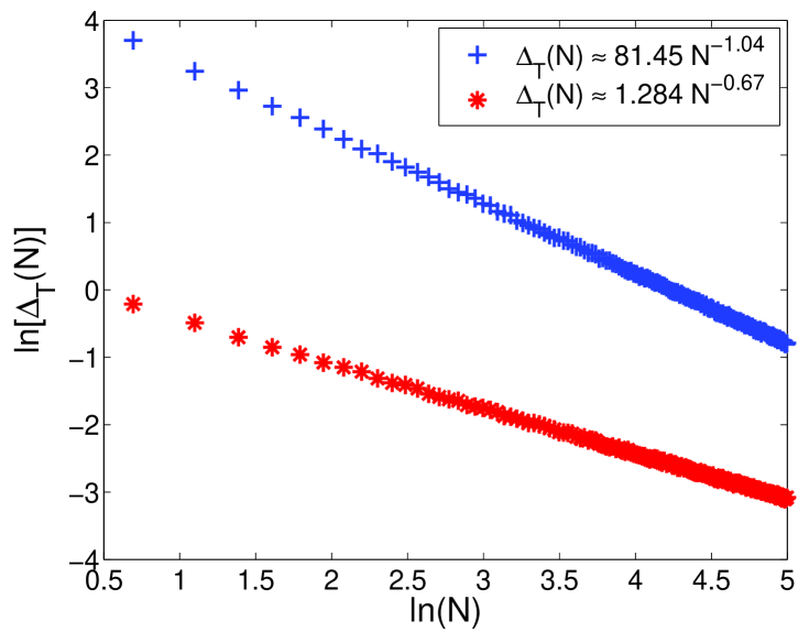
Figure 1: The time-gap variance $\Delta_{T}(N)$ as a function of the sampling size $N$ (in log-log scale). Plus signs and stars represent the variance of average time-gaps for free and congested flows, respectively.

There is, however, one substantial drawback of this description. The time-gap variance was introduced ad hoc and hardly anything is known about its exact mathematical properties in the case of interacting vehicles. It is therefore appropriate to look for an alternative that is mathematically well understood. A natural candidate is the number variance $\Delta_{n}(L)$ that was originally introduced for describing the statistics of eigenvalues in the Random Matrix Theory. It reproduces also the variances in the particle positions of certain class of one-dimensional interacting gases (for example Dyson gas in Ref. [1]).

Consider a set $\{r_{i}:i=1\ldots Q\}$ of distances (i.e. clearances in the traffic terminology) between each pair of cars moving in the same lane. We suppose that the mean distance taken over the complete set is re-scaled to one, i.e.

$$\sum_{i=1}^{Q}r_{i}=Q.$$

Dividing the interval $[0,Q]$ into subintervals $[(k-1)L,kL]$ of a length $L$ and denoting by $n_{k}(L)$ the number of cars in the $k$th subinterval, the average value ${\overline{n}}(L)$ taken over all possible subintervals is

$${\overline{n}}(L)=\frac{1}{\lfloor Q/L\rfloor}\sum_{k=1}^{\lfloor Q/L\rfloor}n_{k}(L)=L,$$

where the integer part $\lfloor Q/L\rfloor$ stands for the number of all subintervals $[(k-1)L,kL]$ included in the interval $[0,Q].$ Number variance $\Delta_{n}(L)$ is then defined as

$$\Delta_{n}(L)=\frac{1}{\lfloor Q/L\rfloor}\sum_{k=1}^{\lfloor Q/L\rfloor}\left(n_{k}(L)-L\right)^{2}$$

and represents the statistical variance of the number of vehicles moving at the same time inside a fixed part of the road of a length $L.$ The mathematical properties of the number variance are well understood. For independent events one gets $\Delta_{n}(L)=L$. Applying it to the highway data in the low density regime (free traffic) one obtains however $\Delta_{n}(L)\approx 5L/6$ (not plotted). The small deviation from the behavior $\Delta_{n}(L)=L$ is induced by the weak (but still nonzero) interaction among the cars.

The situation becomes more tricky when a congested traffic is investigated. The touchy point is that behavior of the number variance is sensitive to the temperature of the underlying gas - or in the terminology of the Random Matrix Theory - to the universality class of the random matrix ensemble. To use the known mathematical results one has not to mix together states with different densities - a procedure known as data unfolding in the Random Matrix Theory. For the transportation this means than one cannot mix together traffic states with different traffic densities and hence with different vigilance of the drivers. So we will perform a separate analysis of the data-samples lying within short density intervals to prevent so the undesirable mixing of the different states.

We divide the region of the measured densities $\varrho\in[0,85~{}\mathrm{veh/km/lane}]$ into eighty five equidistant subintervals and analyze the data from each one of them separately. The number variance $\Delta_{n}(L)$ evaluated with the data in a fixed density interval has a characteristic linear tail (see Fig. 2) that is well known from the Random Matrix Theory. Similarly, such a behavior was found in models of one-dimensional thermodynamical gases with the nearest-neighbor repulsion among the particles (see Ref. [6]). We remind that for the case where the interaction is not restricted to the nearest neighbors but includes all particles the number variance has typically a logarithmical tail - see [1]. So the linear tail of $\Delta_{n}(L)$ supports the view that in the traffic stream the interactions are restricted to the few nearest cars only. The slope of the linear tail of $\Delta_{n}(L)$ decreases with the traffic density (see the top subplot in the Fig. 3). It is a consequence of the increasing alertness of the drivers and hence of the increasing coupling between the neighboring cars in the dense traffic flows.

The fact that the behavior of the number variance evaluated from the traffic data coincides with the results obtained for interacting one-dimensional gases strengthen the idea to apply the equilibrium statistical physics for describing the local properties of the traffic flow. We take the advantage of this approach in a following thermodynamical traffic model.

Consider $N$ identical particles (cars) on a circle of the circumference $N$ exposed to the thermal bath with inverse temperature $\beta.$ Let $x_{i}$ $(i=1\ldots N)$ denote the position of the $i$-th particle and put $x_{N+1}=x_{1}+N,$ for convenience. The particle interaction is described by a potential (see Ref. [3])

$$U\propto\sum_{i=1}^{N}r_{i}^{-1},$$ (2)

where $r_{i}=|x_{i+1}-x_{i}|$ is the distance between the neighboring particles. The nearest-neighbor interaction is chosen with the respect to the realistic behavior of a car-driver in the traffic stream. As published in Ref. [5], the heat bath drives the model into the thermal equilibrium and the probability density $P_{\beta}(r)$ for gap $r$ among the neighboring particles corresponds to the function (1).

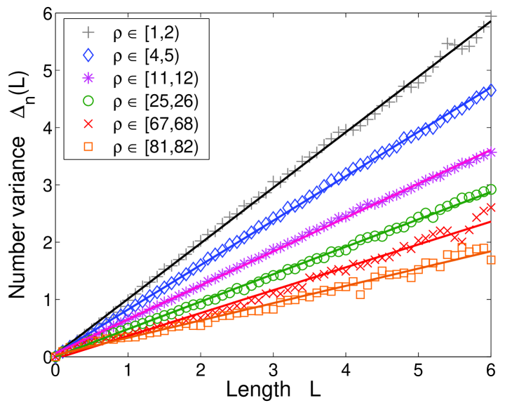
Figure 2: Number variance $\Delta_{n}(L)$ as a function of length $L.$ Plus signs, diamonds, stars, circles, crosses, and squares represent the number variance of real-road data in selected density regions (see legend for details). The curves show the linear approximations of the individual data. Their slopes were carefully analyzed and consecutively visualized on the Fig. 3 (top part).

According to [1], the number variance $\Delta_{n}(L)$ of an one-dimensional gas in thermal equilibrium can be exactly determined from its spacing distribution $P_{\beta}(r).$ For the clearance distribution (1) we obtain (see [10])

$$\Delta_{n}(L)\approx\chi L+\gamma\hskip 28.45274pt(L\rightarrow\infty),$$ (3)

i.e. a linear function with a slope

$$\chi\approx 1+\frac{3-16B\beta-16\sqrt{B\beta}}{\left(3+4\sqrt{B\beta}\right)^{2}}$$

and

$$\gamma\approx\frac{32B\beta\left(21+8B\beta+24\sqrt{B\beta}\right)-48\sqrt{B\beta}-63}{24B\left(3+4\sqrt{B\beta}\right)^{2}},$$

which depend on the inverse temperature $\beta$ only. Above relations represent a large $\beta$ approximations whereas two phenomenological formulae

$$\chi\approx\frac{1}{2.4360~{}\beta^{0.8207}+1}$$

and

$$\gamma\approx\frac{\beta}{5.1926~{}\beta+2.3929}$$

specify the behavior of $\chi$ and $\gamma$ near the origin. We emphasize that, in the limiting case $\beta=0,$ the value of $\chi$ is equal to one, i.e. $\Delta_{n}(L)=L,$ as expected for the independent events. The slope $\chi$ is a decreasing function of $\beta.$

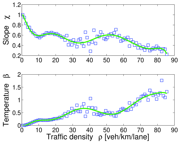
Figure 3: The slope $\chi$ and the inverse temperature $\beta$ as functions of the traffic density $\varrho.$ The squares on the upper subplot display the slope of the number variance $\Delta_{n}(L)$ (see Fig. 2), separately analyzed for various traffic densities. The lower subplot visualizes the fitted values of the inverse temperature $\beta,$ for which the exact form of number variance $\Delta_{n}(L)=\chi(\beta)~{}L+\gamma(\beta)$ corresponds to the number variance obtained from the traffic data. The continuous curves represent a polynomial approximations of the relevant data.

The described properties of the function $\Delta_{n}(L)$ agree with the behavior of the number variance extracted from the traffic data (see Fig. 2). A comparison between traffic data number variance and the formula (3) allows us to determine the empirical dependence of inverse temperature $\beta$ on traffic density $\varrho$. The inverse temperature reflects the microscopic status in which the individual vehicular interactions influence the traffic. Conversely, in the macroscopic approach, traffic is treated as a continuum and modelled by aggregated, fluid-like quantities, such as density and flow (see [7]). Its most prominent result is the dependence of the traffic flow on the traffic density - the fundamental diagram.

It is clear that the macroscopic traffic characteristics are determined by its microscopic status. Consequently there should be a relation between the behavior of the fundamental diagram and that of the inverse temperature $\beta$. On the Figure 4 we display the behavior of the inverse temperature $\beta$ simultaneously with the fundamental diagram. The both curves show a virtually linear increase in the region of a free traffic (up to $\varrho\approx 10~{}\mathrm{veh/km/lane}$). The inverse temperature $\beta$ then displays a plateau for the densities up to $18~{}\mathrm{veh/km/lane}$ while the flow continues to increase. A detailed inspection uncovers, however, that the increase of the traffic flow ceases to be linear and becomes concave at that region. So the flow is reduced with respect to the outcome expected for a linear behavior - a manifestation of the onset of the phenomenon that finally leads to a congested traffic. For larger densities the temperature $\beta$ increases up to $\varrho\gtrapprox 32~{}\mathrm{veh/km/lane}$. The center of this interval is localized at $\varrho\approx 25$ - a critical point of the fundamental diagram at which the flow starts to decrease. This behavior of the inverse temperature is understandable and imposed by the fact that the drivers, moving quite fast in a relatively dense traffic flow, have to synchronize their driving with the preceding car (a strong interaction) and are therefore under a considerable psychological pressure. After the transition from the free to a congested traffic regime (between 40 and $50~{}\mathrm{veh/km/lane}$), the synchronization continues to decline because of the decrease in the mean velocity leading to decreasing $\beta$. Finally - for densities related to the congested traffic - the inverse temperature increases while the flow remains constant. The comparison between the traffic flow and the inverse temperature is even more illustrative when the changes of the flow are taken into account. Therefore we evaluate the derivative of the flow

$$J^{\prime}=\frac{\partial J}{\partial\varrho}$$

and plot the result on the Figure 5. The behavior of the inverse temperature $\beta$ can be understood as a quantitative description of the alertness required by the drivers in a given situation.

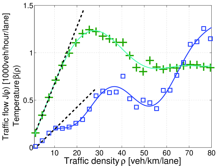
Figure 4: Traffic flow $J(\varrho)$ and inverse temperature $\beta(\varrho)$ as functions of a traffic density $\varrho$. Plus signs display a traffic flow in thousands of vehicles per hour and squares correspond to inverse temperature of the traffic gas. The results of a polynomial curve-fitting are visualized by the continuous curves. The dashed lines represent a linear approximations of the relevant data near the origin.

The dependence of $\beta$ on the density $\varrho$ can be obtained also using the measured clearance distribution and comparing it with the formula (1). It leads to the same results as $\beta$ obtained from the number variance $\Delta_{n}(L)$. It is known (see [1]) that for one-dimensional gases in thermal equilibrium the function $\Delta_{n}(L)$ can be determined from the knowledge of the spacing distribution $P_{\beta}(r).$ So the fact that obtaining $\beta$ by virtue of the number variance $\Delta_{n}(L)$ and the spacing distribution $P_{\beta}(r)$ leads to the same results supports the view that locally the traffic can be described by instruments of equilibrium statistical physics.

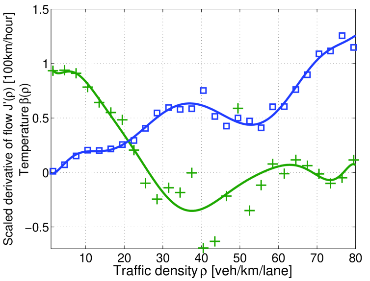
Figure 5: Inverse temperature $\beta(\varrho)$ and scaled derivative of the flow $J^{\prime}=\frac{\partial J}{\partial\varrho}$ as functions of a traffic density $\varrho.$ Squares correspond to the inverse temperature of traffic sample while plus signs display the first derivative of the flow (scaled for better visualization). The continuous curves represent a relevant polynomial approximations.

In summary, we have investigated the statistical variances of the single-vehicle data from the Dutch freeway A9. Particularly, we have separately analyzed the number variance in eighty five equidistant density-subregions and found a linear dependence in each of them. Using the thermodynamical model presented originally in Ref.[3], we have found an excellent agreement between the number variance of particles in thermal-equilibrium and that of the traffic data. It was demonstrated that the inverse temperature of the traffic sample, indicating the degree of alertness of the drivers, shows an increase at both the low and high densities. In the intermediate region, where the free flow regime converts to the congested traffic, it displays more complex behavior.

The presented results support the possibility for applying the equilibrium statistical physics to the traffic systems. It confirms also the hypothesis that short-ranged forwardly-directed power-law potential (2) is a good choice for describing the fundamental interaction among the vehicles.

Acknowledgements

We would like to thank Dutch Ministry of Transport for providing the single-vehicle induction-loop-detector data. This work was supported by the Ministry of Education, Youth and Sports of the Czech Republic within the projects LC06002 and MSM 6840770039.

References

- [1] M.L. Mehta: Random matrices (revised and enlarged), Academic Press, New York (1991)
- [2] D. Helbing and M. Treiber, Phys. Rev. E 68 (2003) 067101.
- [3] M. Krbalek and D. Helbing, Physica A 333 (2004) 370.
- [4] D. Helbing, M. Treiber, and A. Kesting, Physica A 363 (2006) 62.
- [5] M. Krbalek, J. Phys. A 40 (2007) 5813.
- [6] E.B. Bogomolny, U. Gerland, and C. Schmit, Eur. Phys. J. B 19 (2001) 121.
- [7] D. Helbing, Rev. Mod. Phys. 73 (2001) 1067.
- [8] M. Treiber, A. Kesting, and D. Helbing, Physical Review E 74 (2006) 016123.
- [9] P. Wagner, Eur. Phys. J. B 52 (2006) 427.
- [10] M. Krbalek: in preparation