Studies of Stability and Robustness for Artificial Neural Networks and Boosted Decision Trees

Hai-Jun Yang^a,c,∗, Byron P. Roe^a, Ji Zhu^b ^a Department of Physics, University of Michigan, Ann Arbor, MI 48109, USA ^b Department of Statistics, University of Michigan, Ann Arbor, MI 48109, USA ^c Los Alamos National Laboratory, Los Alamos, NM 87545, USA Corresponding author. E-mail address: yhj@umich.edu

Abstract

In this paper, we compare the performance, stability and robustness of Artificial Neural Networks (ANN) and Boosted Decision Trees (BDT) using MiniBooNE Monte Carlo samples. These methods attempt to classify events given a number of identification variables. The BDT algorithm has been discussed by us in previous publications. Testing is done in this paper by smearing and shifting the input variables of testing samples. Based on these studies, BDT has better particle identification performance than ANN. The degradation of the classifications obtained by shifting or smearing variables of testing results is smaller for BDT than for ANN.

keywords:

Boosted Decision Trees; Artificial Neural Networks; Stability; Robustness; Particle Identification; Neutrino Oscillations; MiniBooNE

PACS:

29.85.+c, 02.70.Uu, 07.05.Mh, 14.60.Pq

1 Introduction

The boosting algorithm is one of the most powerful learning techniques introduced during the past decade. The motivation for the boosting algorithm is to design a procedure that combines many “weak” classifiers (such as decision trees, random forests, ANNs etc.) to achieve a powerful classifier. One starts with unweighted training events and builds a decision tree[6]. If a training event is misclassified, then the weight of that event is increased (boosted). A second tree is built using exactly the same set of training events but with new weights. Again misclassified events have their weights boosted and the procedure is repeated several hundred to thousand times until the performance becomes optimal. Each test event is followed through each tree in turn. If it lands on a signal leaf it is given a score of 1, otherwise $-1$ . The sum of the scores from all trees,is the final score of the event. A high score means that the event is most likely signal and a low score that it is most likely background. The major advantages of boosted decision trees are their stability, their ability to handle large numbers of input variables, and their use of boosted weights for misclassified events to give these events a better chance to be correctly classified in succeeding trees.

The Artificial Neural Network (ANN) technique has been widely used in data analysis of High Energy Physics (HEP) experiments in the last decade. The use of the ANN technique usually gives better results than the traditional simple-cut techniques. Based on our previous studies, Boosted Decision Trees (BDT) with the Adaboost[1, 2, 3] or $\epsilon-$ Boost[4, 5] algorithms perform better than ANN and some other boosting algorithms for MiniBooNE particle identification (PID)[6, 7]. More and more major HEP experiments (ATLAS,BaBar,CDF,D0 etc.) [10, 11, 12, 13, 14, 15, 16] have begun to use boosting algorithms as an important tool for data analysis since our first successful application of BDT for MiniBooNE PID[6, 7].

In this paper we discuss the Boosting method in the context of MiniBooNE. For practical applications of data mining algorithms, performance, stability and robustness are determinants. We focus on stability and robustness of ANN and BDT with $\epsilon-$ Boost ( $\epsilon=0.01$ ) by smearing or shifting values of input variables randomly for testing samples. The results obtained in this paper do not represent optimal MiniBooNE PID performance because we only use 30 arbitrarily selected variables for ANN and BDT training and testing. BDT with more input variables results in significantly better performance. However, ANN will not improve significantly by using more input variables [6, 7]. MiniBooNE is a crucial experiment operated at Fermi National Accelerator Laboratory which is designed to confirm or refute the evidence for $\nu_{\mu}\rightarrow\nu_{e}$ oscillations at $\Delta m^{2}\simeq 1eV^{2}$ seen by the LSND experiment[8, 9]. It will imply new physics beyond the Standard Model of particle physics if the LSND signal is confirmed by the MiniBooNE experiment.

2 Training and Testing Samples

The training sample has 50000 signal and 100000 background events. An independent testing sample has 54200 signal and 146600 background events. Fully oscillated $\nu_{e}$ charged current quasi-elastic (CCQE) events are signal; all $\nu_{\mu}$ and non-CCQE intrinsic $\nu_{e}$ events are treated as background. The signature of each event is given by 322 variables[17, 18]. Thirty out of 322 variables were selected randomly for this study. (The selection was by variable name not by the power of the variables.) All selected variables are used for ANN and BDT training and testing.

The detailed description of reconstructed variables is available in MiniBooNE technical notes[17, 18]. Here we briefly mention some of variables used for this study. The MiniBooNE neutrino detector is filled with 800 tons of pure mineral oil, which is contained in a spherical tank of 610-cm inner radius. The detector is divided into two optical isolated regions. The inner region employs 1280 8-inch photomultiplier tubes (PMTs) to measure the charge, time and position of particles produced by neutrino interactions on nuclei. The outer veto region is instrumented with 240 PMTs to tag particles entering or leaving the detector. The final state charged particles passing through the oil can emit both prompt Cherenkov and delayed isotropic scintillation photons, which are detected in a ratio of about 3:1 for $\beta\sim 1$ particles. Some reconstructed variables are listed in the following:

•

fraction of very prompt PMT hits, $-2~{}ns<\Delta T<3~{}ns$
•

fraction of very late PMT hits, $\Delta T>15~{}ns$
•

reconstructed track length
•

angle between track direction and neutrino beam direction
•

ratio of scintillation flux to Cherenkov flux
•

time likelihood in the Cherenkov ring region $0.55<\cos\theta<0.85$
•

time likelihood in $0.4<\cos\theta<0.5$
•

time likelihood in $0.2<\cos\theta<0.4$
•

time likelihood in $-0.2<\cos\theta<0.2$
•

time likelihood in $\cos\theta<-0.2$
•

charge likelihood in various $\cos\theta$ regions
•

reconstructed $\pi^{0}$ mass
•

angle between two $\gamma$ ’s from $\pi^{0}$ decay
•

distance from the first $\gamma$ conversion point to the tank wall
•

the difference of time likelihoods between electron and $\pi^{0}$
•

the difference of charge likelihoods between electron and $\pi^{0}$
•

ratio of measured to predicted charge in $\cos\theta<-0.8$
•

ratio of measured to predicted charge in $0.5<\cos\theta<0.7$
•

for the two $\gamma$ hypothesis, the fraction of Cherenkov flux in the lower energy $\gamma$

The time (charge) likelihood is the likelihood of the time (charge) distribution of the PMT hits under the given hypothesis.

2.1 Training Samples

We prepared 10 statistically independent training samples. Each sample has 5000 signal and 10000 background events selected sequentially from the large training sample. Both ANN and BDT are trained separately on each of these training samples. For a given testing sample, then, ANN and BDT each have 10 sets of results. The mean values and variance of the 10 sets of results are calculated to compare the ANN and BDT methods.

2.2 Testing Samples Set 1 - Smearing Randomly

In order to study the stability of ANN and BDT on the testing samples, we randomly smear the input variables by 1%, 3%, 5%, 8% and 10%, respectively. The smearing formula is written as

V^{j}_{i}=V^{j}_{i}\times(1+sf\times R^{j}_{i})

where $V^{j}_{i}$ represents value of $j$ -th variable in $i$ -th testing event, $sf$ is the smearing factor (= 0, 0.01, 0.03, 0.05, 0.08, 0.1). $R^{j}_{i}$ is a random number with a Gaussian distribution; it is different for each variable and each event.

2.3 Testing Samples Set 2 - Shifting Randomly

The random shift formula can be written as

V^{j}_{i}=V^{j}_{i}\times(1+sf\times R^{j}_{i})

where $V^{j}_{i}$ represents value of $j$ -th variable in $i$ -th testing event, $sf$ is the shifting factor (= 0, 0.01, 0.03, 0.05, 0.08, 0.1) and $R^{j}_{i}$ is a discrete random number with value 1 or $-1$ .

2.4 Testing Samples Set 3 - Shifting Positively

The values of all training variables are shifted positively. The formula is,

V^{j}_{i}=V^{j}_{i}\times(1+sf)

where $V^{j}_{i}$ represents value of $j$ -th variable in $i$ -th testing event, $sf$ is the shifting factor (= 0, 0.01, 0.03, 0.05, 0.08, 0.1).

2.5 Testing Samples Set 4 - Shifting Negatively

The values of all training variables are shifted negatively. The formula is,

V^{j}_{i}=V^{j}_{i}\times(1-sf)

where $V^{j}_{i}$ represents value of $j$ -th variable in $i$ -th testing event, $sf$ is the shifting factor (= 0, 0.01, 0.03, 0.05, 0.08, 0.1).

2.6 Testing Samples Set 5 - Shifting Mix

Each variable is shifted in one direction for all testing events. The shift direction for each variable is determined by a random number with the discrete values of 1 or $-1$ .. The formula is written as,

V^{j}_{i}=V^{j}_{i}\times(1+sf\times R^{j})

where $V^{j}_{i}$ represents value of $j$ -th variable in $i$ -th testing event, $sf$ is the shifting factor (= 0, 0.01, 0.03, 0.05, 0.08, 0.1).

3 Results

All ANN and BDT results shown in this paper are from testing samples.

3.1 Results from original testing samples

Table 1 lists the signal and background efficiencies for ANN and BDT with root mean square (RMS) errors and statistical errors for background efficiencies. The efficiency ratio is defined as background efficiency from ANN divided by that from BDT using the original testing sample (no smearing and shifting) and the same signal efficiency. Efficiency ratio values greater than 1 mean that BDT works better than ANN by suppressing more background events (less background efficiency) for a given signal efficiency. From Table 1, the efficiency ratios vary from about 1.12 to 1.75 for signal efficiencies ranging from 90% to 30%. Lower signal efficiencies yield higher ratio values. The statistical error of the test background efficiency for ANN is slightly higher than that for BDT depending on the signal efficiency. The variance of 10 test background efficiencies for ANN trained with 10 randomly selected training samples is about $2\sim 5$ times larger than that for BDT. This result indicates that BDT training performance is more stable than ANN training.

3.2 Results from smeared testing samples

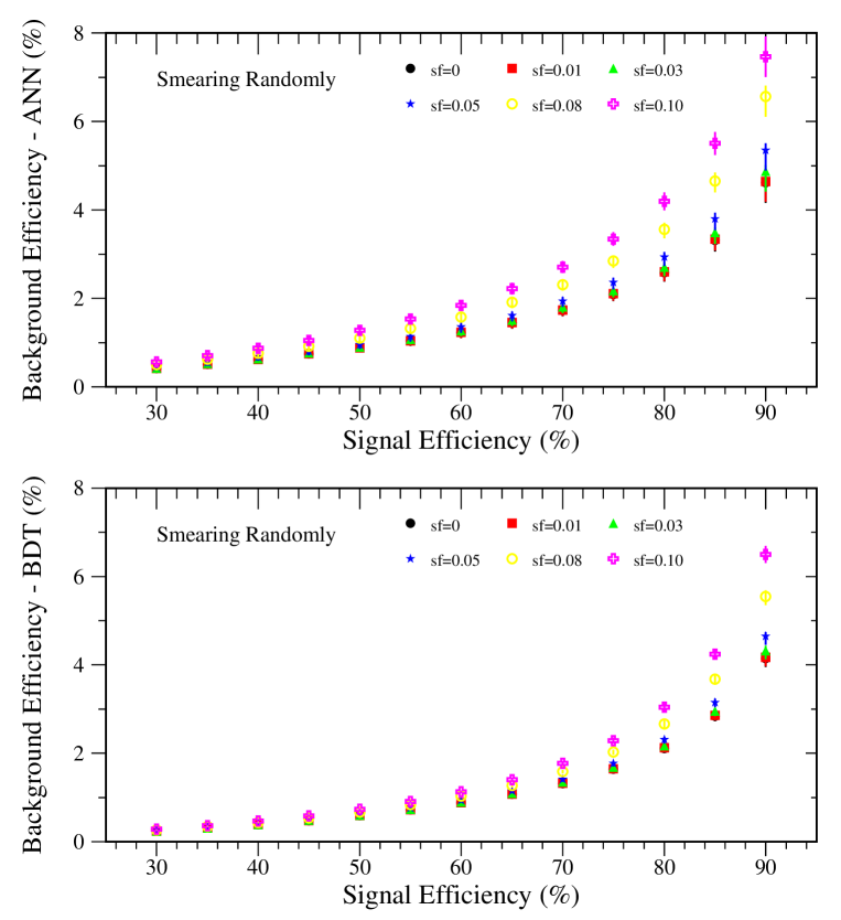
The background efficiency versus signal efficiency for the smeared testing sample set 1 is shown in Figure 1. The top plot shows results from ANN, the bottom plot shows results from BDT. Dots are for the results from the testing sample without smearing, boxes, triangles, stars, circles and crosses are for results from testing samples with 1%, 3%, 5%, 8% and 10% smearing, respectively. Both ANN and BDT are quite stable for testing samples which are randomly smeared within 5%, typically within about 5%-12% performance decrease for BDT and 7% - 16% decrease for ANN as shown in Figure 1. For the 10% smeared testing sample, however, the performance of ANN is degraded by 37% to 62%; higher signal efficiency results have larger degradation. The corresponding performance of BDT is degraded by 19% to 57%.

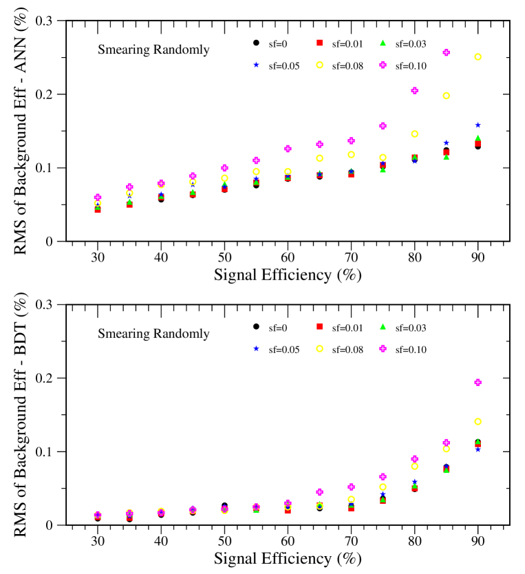
The variance (RMS) of background efficiencies based on trials versus signal efficiency for the 10 different smeared testing samples is shown in Figure 2. The variance of background efficiencies from BDT is about $2\sim 5$ times smaller than that from ANN as presented in the bottom plot of Figure 3. The variance ratios between ANN and BDT remain reasonably stable for various testing samples with different smearing factors.

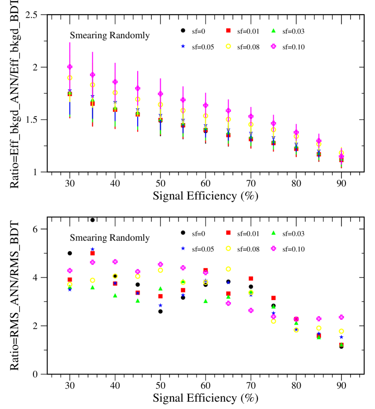
Figure 3 shows the ratio of background efficiency from ANN and BDT versus signal efficiency (top plot) and the ratio of RMS of background efficiency from ANN and BDT versus signal efficiency (bottom plot). Dots are for results from the testing sample without smearing; boxes, triangles, stars, circles and crosses are for results from 1%, 3%, 5%, 8% and 10% smearing, respectively. Error bars in the top plot are for RMS errors of ratios which are calculated by propagating errors from the RMS errors from ANN and BDT results. The performance of BDT ranges from 12% to 75% better than that of ANN, depending on the signal efficiency as shown in the top plot of Figure 3. The ratio of background efficiency from ANN and BDT increases with an increase in the smearing factor. For the testing sample with 10% random smearing, the efficiency ratio increases about 15%. This result indicates that the BDT is more stable than ANN for this set of specific testing samples with random smearing.

Figure 4 shows the background efficiency versus smearing factor for three given signal efficiencies 30%(dots) , 50%(boxes) and 70%(triangles). The top plot of Figure 4 shows results from ANN. The bottom plot of Figure 4 shows results from BDT. The performance of ANN and BDT degrade modestly with relatively small smearing factors $>\sim$ 0.03. Larger smearing factors result in significant performance degradation of ANN and BDT.

3.3 Results from shifted testing samples

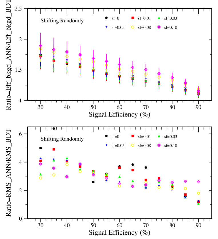
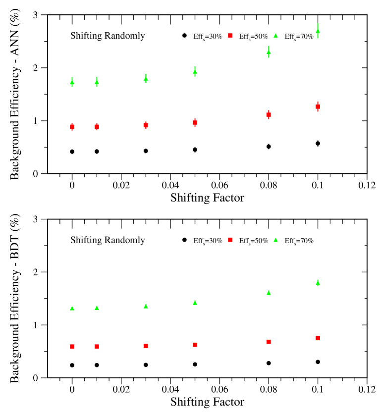
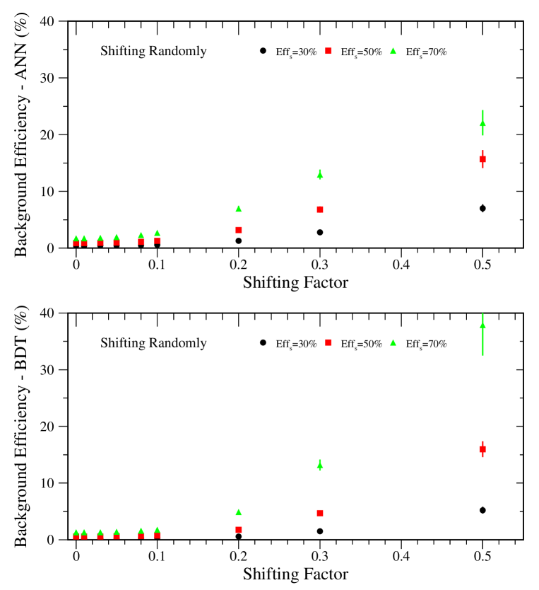
Figure 5 shows the ratio of background efficiency from ANN and BDT versus signal efficiency (top plot) and the ratio of variance of background efficiency from ANN and BDT versus signal efficiency (bottom plot) for the testing samples of set 2 with random shifting. Figure 6 shows the background efficiency versus smearing factor, for ANN (top plot) and BDT (bottom plot). Resutls from the randomly shifted testing samples of set 2 are comparable to those from the randomly smeared testing samples of set 1. In order to estimate the dependence of ANN and BDT performance on the factor of random shifting, we vary the shifting factor from 0 to 0.5, as shown in Figure 7. Both ANN and BDT performance degrade significantly by randomly shifting the input variables with large shifting factor( $>$ 0.1).

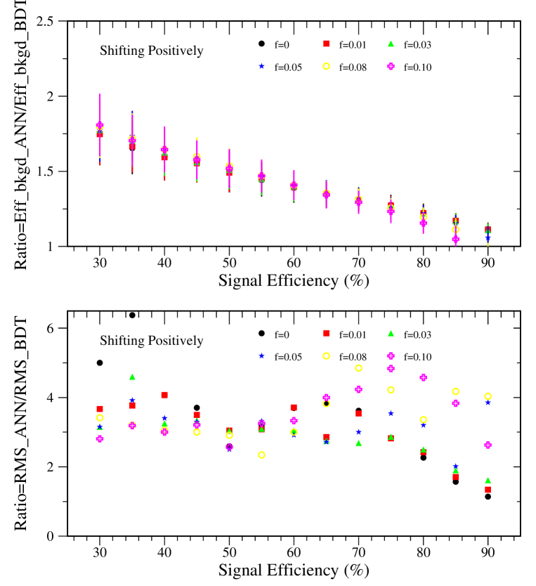
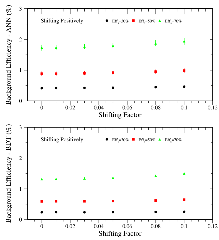
Figure 8 shows the ratio of background efficiency from ANN and BDT versus signal efficiency (top plot) and the ratio of variance of background efficiency from ANN and BDT versus signal efficiency (bottom plot) for the testing samples of set 3 with overall positive shifting. Figure 9 shows the background efficiency versus smearing factor, for ANN (top plot) and BDT (bottom plot). The results are reasonably stable for both ANN and BDT versus shifting factor.

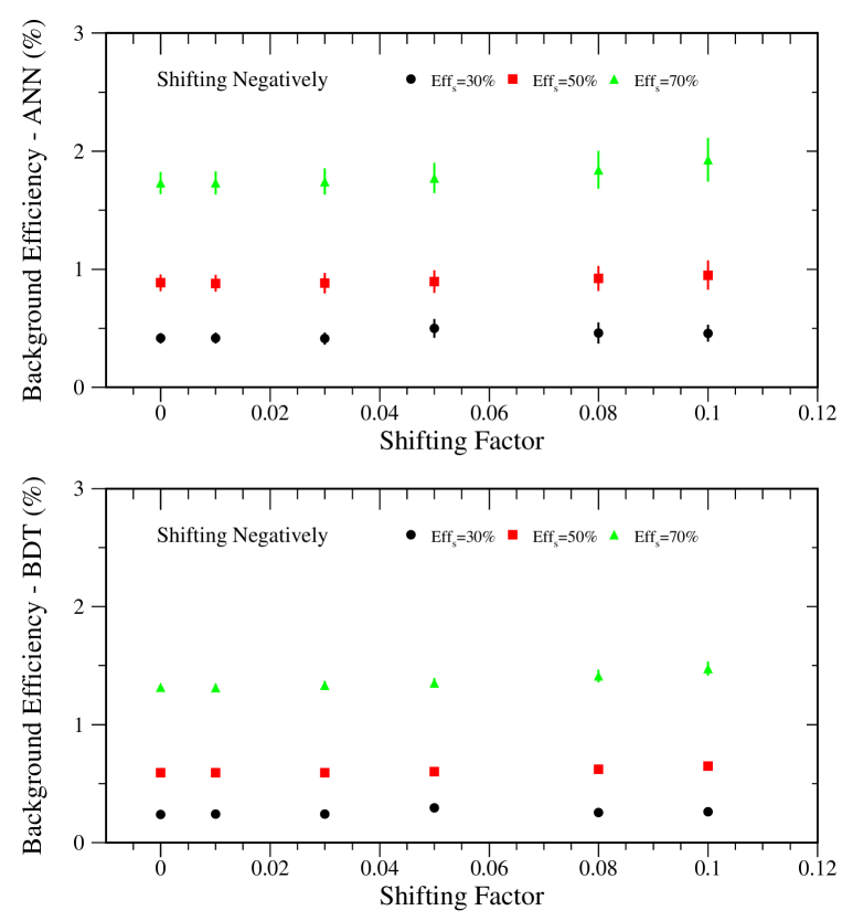
Figure 10 shows the ratio of background efficiency from ANN and BDT versus signal efficiency (top plot) and the ratio of variance of background efficiency from ANN and BDT versus signal efficiency (bottom plot) for the testing samples of set 4 with overall negative shifting. Figure 11 shows the background efficiency versus smearing factor, for ANN (top plot) and BDT (bottom plot). The results are remain reasonably stable for both ANN and BDT versus shifting factor.

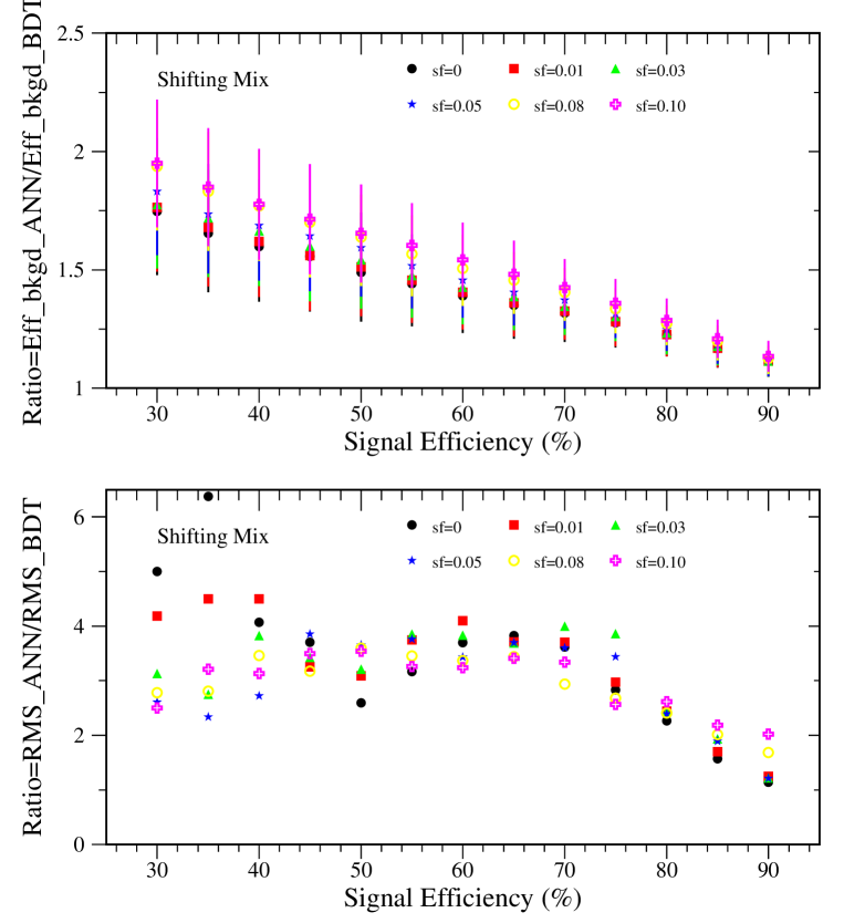
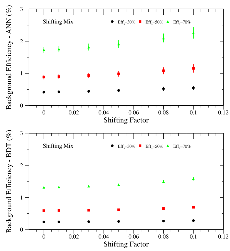
Figure 12 shows the ratio of background efficiency from ANN and BDT versus signal efficiency (top plot) and the ratio of variance of background efficiency from ANN and BDT versus signal efficiency (bottom plot) for the testing samples of set 5 with random positive or negative shifting. Figure 13 shows the background efficiency versus smearing factor, for ANN (top plot) and BDT (bottom plot).

3.4 Further Validation

In order to make a cross check, a new set of 30 out of the 322 particle identification variables were selected and the whole analysis was redone. Most results are quite similar to the results obtained in Sections 3.1–3.3. BDT, again, was more stable than ANN. However, the second set of 30 variables overall was less powerful by a factor of about 2 than the first set. Because of this, the variances were dominated more by the random variations than the variations due to a change in power with smearing or shifting. The variances of the second set were only about half the variances of the first set, but exhibited much more random behavior.

4 Conclusions

The performance, stability and robustness of ANN and BDT were compared for particle identification using the MiniBooNE Monte Carlo samples. BDT has better particle identification performance than ANN, even using only 30 PID variables. The BDT performance relative to that of ANN depends on the signal efficiency. The variance in background efficiencies of testing results due to various BDT trainings is smaller than those from ANN trainings regardless of testing samples with or without smearing and shifting. The performance of both BDT and ANN are degraded by smearing and shifting the input variables of the testing samples. ANN degrades more than BDT depending on the signal efficiency based on MiniBooNE Monte Carlo samples.

5 Acknowledgments

We wish to express our gratitude to the MiniBooNE collaboration for the excellent work on the Monte Carlo simulation and the software package for physics analysis. This work is supported by the Department of Energy and by the National Science Foundation of the United States.

References

[1] Y. Freund and R.E. Schapire (1996), Experiments with a new boosting algorithm. Proc COLT, 209–217. ACM Press, New York (1996).
[2] Y. Freund and R.E. Schapire, A short introduction to boosting, Journal of Japanese Society for Artificial Intelligence, 14(5), 771-780, (September, 1999).
[3] R.E. Schapire, The boosting approach to machine learning: An overview, MSRI Workshop on Nonlinear Estimation and Classification, (2002).
[4] J. Friedman (2001), Greedy function approximation: a gradient boosting machine, Annals of Statistics, 29:5.
[5] J. Friedman, Recent Advances in Predictive Machine Learning, Proceedings of Phystat2003, Stanford U., (Sept. 2003).
[6] B.P. Roe, H.J. Yang, J. Zhu, Y. Liu, I. Stancu, G. McGregor, Boosted decision trees as an alternative to artificial neural network for particle identification, Nucl.Instrum.Meth. A543(2005) 577-584, physics/0408124.
[7] H.J. Yang, B.P. Roe, J. Zhu, Studies of boosted decision trees for MiniBooNE Particle Identification Nucl.Instrum.Meth. A555(2005) 370-385, physics/0508045.
[8] E. Church et al., BooNE Proposal, FERMILAB-P-0898(1997).
[9] A. Aguilar et al., Phys. Rev. D 64(2001) 112007.
[10] J. Conrad and F. Tegenfeldt, Applying Rule Ensembles to the Search for Super-Symmetry at the Large Hadron Collider, JHEP 0607040(2006), hep-ph/0605106.
[11] I. Narsky, StatPatternRecognition: A $C^{++}$ Package for Statistical Analysis of High Energy Physics Data, physics/0507143.
[12] I. Narsky, Optimization of Signal Significance by Bagging Decision Trees, physics/0507157.
[13] BaBar Collaboration, Measurement of CP-violation asymmetries in the $B^{0}\rightarrow K^{+}K^{-}K^{0}$ Dalitz plot, hep-ex/0607112.
[14] M.L. Yu, M.M. Xu, L.S. Liu, An Empirical study of boosted neural network for particle classification in high energy collisions, hep-ph/0606257.
[15] P.M. Perea, Search for t-Channel Single Top Quark Production in ppbar Collisions at 1.96 TeV, FERMILAB-THESIS-2006-15.
[16] A. Hocker, J. Stelzer, H. Voss, K. Voss, X Prudent, Toolkit for Parallel Multivariate Data Analysis, http://tmva.sourceforge.net/. http://root.cern.ch/root/html512/TMVA__MethodBDT.html
[17] Y. Liu and I. Stancu, BooNE-TN-36, 09/15/2001; BooNE-TN-50, 02/18/2002; BooNE-TN-100, 09/19/2003; BooNE-TN-141, 08/25/2004; BooNE-Memoxx, 08/03/2005; BooNE-TN-178, 03/01/2006.
[18] B.P. Roe and H.J. Yang, BooNE-TN-117, 03/18/2004; BooNE-TN-147, 11/18/2004; BooNE-TN-151, 01/08/2005; BooNE-Memo24, 08/10/2005; BooNE-TN-189, 7/10/2006.

Eff_signal (%)	Eff_bkgd_ANN (%)	Eff_bkgd_BDT (%)	Ratio = Eff_bkgd_ANN
	$\pm~{}\sigma_{RMS}$	$\pm~{}\sigma_{RMS}$	/ Eff_bkgd_BDT
30	0.416 $\pm$ 0.045	0.238 $\pm$ 0.009	1.748 $\pm$ 0.201
35	0.512 $\pm$ 0.051	0.310 $\pm$ 0.008	1.655 $\pm$ 0.172
40	0.623 $\pm$ 0.057	0.389 $\pm$ 0.014	1.599 $\pm$ 0.157
45	0.748 $\pm$ 0.063	0.481 $\pm$ 0.017	1.557 $\pm$ 0.142
50	0.885 $\pm$ 0.070	0.594 $\pm$ 0.027	1.489 $\pm$ 0.136
55	1.041 $\pm$ 0.076	0.722 $\pm$ 0.024	1.441 $\pm$ 0.116
60	1.227 $\pm$ 0.085	0.882 $\pm$ 0.023	1.391 $\pm$ 0.102
65	1.449 $\pm$ 0.088	1.074 $\pm$ 0.023	1.350 $\pm$ 0.088
70	1.732 $\pm$ 0.094	1.315 $\pm$ 0.026	1.317 $\pm$ 0.076
75	2.095 $\pm$ 0.102	1.643 $\pm$ 0.036	1.276 $\pm$ 0.068
80	2.585 $\pm$ 0.111	2.110 $\pm$ 0.049	1.225 $\pm$ 0.060
85	3.316 $\pm$ 0.124	2.842 $\pm$ 0.079	1.167 $\pm$ 0.054
90	4.618 $\pm$ 0.129	4.143 $\pm$ 0.113	1.115 $\pm$ 0.044

Table 1: Signal and background efficiencies for ANN and BDT with RMS errors for background efficiencies. The ratio is defined as the background efficiency from ANN divided by that from BDT using the original testing sample (no smearing and shifting) and the same signal efficiency.

Refer to caption — Figure 1: Background efficiency versus signal efficiency. The top plot shows results from ANN with smeared testing samples set 1. The bottom plot shows results from BDT. Dots are for the testing sample without smearing; boxes, triangles, stars, circles and crosses are for 1%, 3%, 5%, 8% and 10% smearing, respectively.