Seismic motion in urban sites consisting of blocks in welded contact with a soft layer overlying a hard half space: II. large and infinite number of identical equispaced blocks

Abstract

We address the problem of the response to a seismic wave of an urban site consisting of a large and infinite number ($N_{b}$) of identical, equispaced blocks overlying a soft layer underlain by a hard substratum. The results of the theoretical analysis, appealing to a space-frequency mode-matching (MM) technique, are compared to those obtained by a space-time finite element (FE) method. The two methods are shown to give rise to much the same prediction of seismic response for $N_{b}=10$. The MM technique is also applied to the case $N_{b}=\infty$, notably to reveal the structure and natural frequencies of the vibration modes of the urban site. The mechanism of the interaction between blocks and the ground, as well as that of the collective effects of the blocks, are studied. It is shown that the presence of a large number of blocks modifies the seismic disturbance in a manner which evokes, and may partially account for, what was observed during many earthquakes in Mexico City. Disturbances at a much smaller level, induced by a small number of blocks are studied in the companion paper.

Keywords: Duration, amplification, seismic response, cities.

Abbreviated title: Seismic response in quasi-periodic and periodic urban sites

Corresponding author: Armand Wirgin, tel.: 33 4 91 16 40 50, fax: 33 4 91 16 42 70, e-mail: wirgin@lma.cnrs-mrs.fr

1 Introduction

The Michoacan earthquake that struck Mexico City in 1985 presented some particular characteristics which have since been encountered at the same site and at various other urban sites [32, 25, 27, 22], but usually at a smaller scale. Other than the fact that the response in downtown Mexico varied considerably in a spatial sense [14, 33], was quite intense and of very long duration at certain locations (as much as $\approx$3min [30, 33, 15]), and often took the form of a quasi-monochromatic signal with beatings [28, 33], a remarkable feature of this earthquake (studied in [15, 6, 18, 19]) was that such strong motion could be caused by a seismic source so far from the city (the epicenter was located in the subduction zone off the Pacific coast, approximately 350km from Mexico City). It is now recognized [6, 7] that the characteristics of the abnormal response recorded in downtown Mexico were partially present in the waves entering into the city (notably $60$km from the city as recorded by the authors of [15]) after having accomplished their voyage from the source, this being thought to be due to the excitation of Love and generalized-Rayleigh modes by the irregularities of the crust [6, 9, 15]).

In the present investigation (as well as in the companion paper), we focus on the the presence of the built features of the urban site as a complementary explanation of the abnormal response. In the companion paper, we treat the case of one or two (different or identical) built features in the form of cylindrical blocks. Herein, we study the case of many (10, 20, 40,…., $\infty$) identical blocks. Such a configuration is a more realistic representation of a real city due to the large number of blocks it incorporates, but the assumptions that the blocks are: i) cylindrical, ii) identical and iii) periodically arranged, are rather far removed from reality, except in restricted portions of modern cities and megacities. Nevertheless, these assumptions are not more unrealistic than random dispositions of blocks with random sizes [10, 34, 17] and compositions, and have the advantage of enabling a theoretical analysis which can shed some light on the physical origins of the above-mentioned exotic phenomena.

The periodic model of cities built on sites with a soft layer overlying a hard substratum solicited by seismic waves originated in the work of Wirgin and Bard [38]. Unfortunately, the theoretical apparatus underlying the numerical results was not given in this paper (only references were made to studies that treat this issue, but as most of these references were relative to problems of electromagnetic waves, they have escaped the attention of the civil engineering and geophysical communities) and the distance between blocks in the computational results was taken to be 2000m, which, in our present opinion, is unrealistically large (unless the blocks represent skyscrapers, of which there are usually few, and largely-distant one from the other).

The object of the present investigation is thus twofold: i) give the missing theoretical foundations of the results of [38], and ii) treat cities that are more realistic than those in [38] and in the companion paper. More specifically, we shall address the following questions:

(i) how should one account for the principal features of the seismic response in the cases of a relatively-large number of blocks (the case of a relatively small number of blocks being treated in the companion paper)?

(ii) what are the vibrational modes of the global structures (i.e. the superstructure plus the geophysical structure) and what are the mechanisms of their excitation and interaction?

(iii) what are the repercussions of resonant phenomena on the seismic response?

(iv) what are the differences in seismic response between configurations with a small and a large number of blocks?

2 Candidate sites

Many earthquake-prone cities and megacities (New Delhi, Tokyo, Mexico City, Istanbul, San Francisco, Basel, etc.) are built on soft soil underlain by a hard substratum and contain districts with periodic, or nearly-periodic arrangements of blocks or buildings. An attempt will be made in the present investigation to analyze the seismic response of districts of this type in the two cities, Mexico City and Nice (satellite pictures of which are depicted in figs. 1 and 2 respectively).

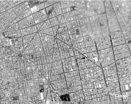
Figure 1: Satellite picture of a portion of Mexico City, Mexico.

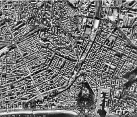
Figure 2: Satellite picture of a portion of Nice, France.

3 Description of the configurations

We focus on a portion of a city characterized by a periodic or quasi-periodic set of identical blocks, assumed to have 2D geometry, with $x_{3}$ the ignorable coordinate of a $Ox_{1}x_{2}x_{3}$ cartesian coordinate system (see fig. 3).

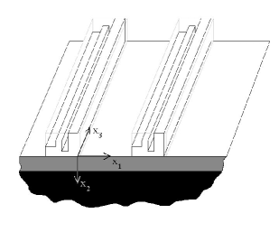
Figure 3: View of the 2D city (only two of the blocks are represented).

The blocks are in welded contact with the ground underneath which is located a horizontal soft layer underlain by a hard half space (see fig. 3). Each block is composed of one or more buildings, all the blocks have the same shape (rectangular in the cross-section plane), are of the same size (characterized by two constants, their height $b$ and width $w$) and composition, and their separation (center-to-center spacing) is a constant $d$. For the purpose of the analysis, each block is homogenized, so that the final geometry of the city is as represented in fig. 4.

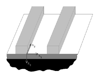
Figure 4: View of the 2D city with homogenized blocks (only two of the blocks are represented).

Fig. 5 represents a cross-section (sagittal plane) view of the city.

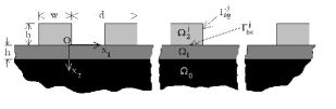
Figure 5: Sagittal plane view of the 2D city with a set of identically, equally-spaced, homogenized blocks.

$\Gamma_{f}$ is the stress-free surface composed of a ground portion $\Gamma_{g}$, assumed to be flat and horizontal, and a portion $\Gamma_{ag}$, constituting the reunion of the above-ground-level boundaries $\Gamma_{ag}^{j}~{};~{}j\in\mathbb{Z}$ of the blocks. The ground $\Gamma_{G}$ is flat and horizontal, and is the reunion of $\Gamma_{g}$ and the base segments $\Gamma_{bs}^{j}~{};~{}j\in\mathbb{Z}$ joining the blocks to the underground.

The medium in contact with, and above, $\Gamma_{f}$ is air, assumed to be the vacumn (i.e., $\Gamma_{f}$ is stress-free). The medium in contact with, and below $\Gamma_{G}$ is the mechanically-soft layer occupying the domain $\Omega_{1}$, which is laterally-infinite and of thickness $h$, and whose lower boundary is $\Gamma_{h}$, assumed to be flat and horizontal. The soft material in the layer is in welded contact across $\Gamma_{h}$ with the mechanically-hard material in the semi-infinite domain (substratum) $\Omega_{0}$.

The domain of the $j$-th block is denoted by $\Omega_{2}^{j}$ and the reunion of all the $\Omega_{2}^{j}~{};~{}j\in\mathbb{B}$ is denoted by $\Omega_{2}$. The material in each block is in welded contact with the material in the soft layer across the base segments $\Gamma_{bs}^{j}~{};~{}j\in\mathbb{Z}$.

The origin $O$ of the cartesian coordinate system is on the ground, $x_{2}$ increases with depth and $x_{3}$ is perpendicular to the (sagittal) plane in figs. 3-5. With $\mathbf{i}_{j}$ the unit vector along the positive $x_{j}$ axis, we note that the unit vectors normal to $\Gamma_{G}$ and $\Gamma_{h}$ are $-\mathbf{i}_{2}$.

The media filling $\Omega_{0}$, $\Omega_{1}$ and $\Omega_{2}^{j}$ are $M^{0}$, $M^{1}$ and $M^{2j}=M^{2}~{};~{}\forall j\in\mathbb{B}$ respectively and the latter are assumed to be initially stress-free, linear, isotropic and homogeneous (thus, each block, which is generally inhomogeneous, is assumed to be homogenized in our analysis). We assume that $M^{0}$ is non-dissipative whereas $M^{1}$ and $M^{2}$ are dissipative.

The seismic disturbance is delivered to the site in the form of a shear-horizontal (SH) plane pulse wave, initially propagating in $\Omega_{0}$. The SH nature of the incident wave (which fact is indicated by the superscript $i$ in the following) means that the motion associated with it is strictly transverse (i.e., in the $x_{3}$ direction and independent of the $x_{3}$ coordinate). Both the SH polarization and the invariance of the incident wave with respect to $x_{3}$ are communicated to the fields that are generated at the site in response to the incident wave. Thus, our analysis will deal only with the propagation of 2D SH waves (i.e., waves that depend exclusively on the two cartesian coordinates $x_{1},~{}x_{2}$ and that are associated with motion in the $x_{3}$ direction only).

We shall be concerned with a description of the elastodynamic wavefield on the free surface (i.e., on $\Gamma_{f}$) resulting from plane seismic wave solicitation of the site.

4 Governing equations

4.1 Space-time framework wave equations

In a generally-inhomogeneous, isotropic elastic or viscoelastic medium $M$ occupying $\mathbb{R}^{3}$, the space-time framework wave equation for SH waves is:

$$\nabla\cdot(\mu(\mathbf{x},\omega)\nabla u(\mathbf{x},t))-\rho(\mathbf{x})\partial_{t}^{2}u(\mathbf{x},t)=-\rho(\mathbf{x})f(\mathbf{x},t)~{},$$ (1)

wherein $u$ is the displacement component in the $\mathbf{i}_{3}$ direction, $f$ the component of applied force density in the $\mathbf{i}_{3}$ direction, $\mu$ the Lamé descriptor of rigidity, $\rho$ the mass density, $t$ the time variable, $\omega$ the angular frequency, $\partial^{n}_{t}$ the $n-$th partial derivative with respect to $t$, and $\mathbf{x}=(x_{1},x_{2})$. Since our configuration involves three homogeneous media and the solicitation takes the form of a plane wave initially propagating in $\Omega_{0}$ (thus, the source density is nil for this type of wave), we have

$$\left(c^{m}(\omega)\right)^{2}\nabla\cdot\nabla u^{m}(\mathbf{x},t)-\partial_{t}^{2}u^{m}(\mathbf{x},t)=0~{}~{};~{}~{}\mathbf{x}\in\Omega_{m}~{};~{}m=0,1,2j~{}~{},~{}j\in\mathbb{B}~{},$$ (2)

wherein $m$ superscripts designate the medium (0 for $M^{0}$, etc.), and $c^{m}$ is the generally-complex velocity of shear body waves in $M^{m}$, related to the density and rigidity by

$$\left(c^{m}(\omega)\right)^{2}=\frac{\mu^{m}(\omega)}{\rho^{m}}~{},$$ (3)

it being understood that $\rho^{m},\mu^{m}(\omega)~{};~{}m=0,1,2j,~{}j\in\mathbb{B}$ are constants with respect to $\mathbf{x}$. In addition, the densities are positive real, and we assume that the substratum is a dissipation-free solid so that the rigidity therein is a positive real constant with respect to $\omega$, i.e., $\mu^{0}(\omega)=\mu^{0}>0$.

4.2 Space-frequency framework wave equations

The space-frequency framework versions of the wave equations (2) are obtained by expanding the displacements in Fourier integrals:

$$u^{m}(\mathbf{x},t)=\int_{-\infty}^{\infty}u^{m}(\mathbf{x},\omega)e^{-\mbox{i}\omega t}d\omega~{},\forall t\in\mathbb{R}~{},$$ (4)

(wherein $\mbox{i}=\sqrt{-1}$, $\omega$ the angular frequency and $t$ the time) so as to give rise to the Helmholtz equations

$$\nabla\cdot\nabla u^{m}(\mathbf{x},\omega)+\left(k^{m}(\omega)\right)^{2}u^{m}(\mathbf{x},\omega)=0~{}~{};~{}~{}\forall\mathbf{x}\in\Omega_{m}~{}~{};~{}~{}m=0,1~{},2j,~{}j\in\mathbb{B}~{},$$ (5)

wherein

$$k^{m}(\omega):=\frac{\omega}{c^{m}(\omega)}=\omega\sqrt{\frac{\rho^{m}}{\mu^{m}(\omega)}}~{}.$$ (6)

is the generally-complex wavenumber in $M^{m}$.

We shall deal with constant quality factors $Q^{m}~{};~{}m=1,2$ over the frequency range of solicitation, so that the frequency-dependent rigidities take the form given in [26],

$$\mu^{m}(\omega)=\mu^{m}_{ref}\left(\frac{-\mbox{i}\omega}{\omega_{ref}}\right)^{\frac{2}{\pi}\arctan\left(\frac{1}{Q^{m}}\right)}~{};~{}m=1,2~{},$$ (7)

wherein: $\omega_{ref}$ is a reference angular frequency, chosen herein to be equal to $9\times 10^{-2}$Hz. Hence

$$c^{m}(\omega)=c^{m}_{ref}\left(\frac{-\mbox{i}\omega}{\omega_{ref}}\right)^{\frac{1}{\pi}\arctan\left(\frac{1}{Q^{m}}\right)}~{};~{}m=1,2~{},$$ (8)

with $c^{m}_{ref}:=\sqrt{\frac{\mu^{m}_{ref}}{\rho^{m}}}$. Even though $Q^{m}~{},~{}m=1,2$ are non-dispersive (i.e., do not depend on $\omega$) under the present assumption, the phase velocities $c^{m}~{};~{}m=1,2$ are dispersive.

Due to the assumptions made in sect. 3:

$$k^{0}(\omega):=\frac{\omega}{c^{0}}=\omega\sqrt{\frac{\rho^{0}}{\mu^{0}}}~{},$$ (9)

(i.e., $Q^{0}=\infty$ so that $k^{0}$ is real).

4.3 Space-frequency and space-time framework expressions of the incident plane wave

As mentioned above, we shall be concerned with plane wave excitation of the city.

Actually, a plane wave satisfies the homogeneous wave equation in the space-time framework and a homogeneous Helmholtz equation in the space-frequency framework.

The field is chosen to take the form of a pseudo Ricker-type pulse in the space-time framework, whose shape is directly connected with the site we will consider in the numerical application (either a Nice-like site, or a Mexico city -like site) .

4.3.1 Space-frequency-framework representation of the plane, impulsive, incident wave

The plane wave nature of the incident wave is embodied in the choice

$$u^{i}(\mathbf{x},\omega)=S(\omega)\exp\left[\mbox{i}k^{0}\left(x_{1}s^{i}-x_{2}c^{i}\right)\right]~{},$$ (10)

wherein $s^{i}=\sin\theta^{i}$, $c^{i}=\cos\theta^{i}$ and $\theta^{i}$ is the angle of incidence in the $x_{1}-x_{2}$ plane with respect to the $x_{2}$ axis.

The fact that the incident wave is a pseudo Ricker pulse means that the amplitude spectrum $S(\omega)$ is given by

$$S(\omega)=\frac{1}{\sqrt{\pi}}\frac{\omega^{2}}{4\alpha^{3}}\exp\left(\mbox{i}t_{s}\omega-\frac{\omega^{2}}{4\alpha^{2}}\right)~{},$$ (11)

to which corresponds the temporal variation (Fourier inverse of $S(\omega)$):

$$S(t)=-\left[2\alpha^{2}(t_{s}-t)^{2}-1\right]\exp\left[-\alpha^{2}(t_{s}-t)^{2}\right]~{},$$ (12)

for Nice-like site solicitation and by

$$S(\omega)=-\frac{2\alpha^{2}}{\sqrt{\pi}}\frac{\omega^{2}}{4\alpha^{3}}\exp\left(\mbox{i}t_{s}\omega-\frac{\omega^{2}}{4\alpha^{2}}\right)~{},$$ (13)

to which corresponds the temporal variation (Fourier inverse of $S(\omega)$):

$$S(t)=2\alpha^{2}\left[2\alpha^{2}(t_{s}-t)^{2}-1\right]\exp\left[-\alpha^{2}(t_{s}-t)^{2}\right]~{},$$ (14)

for the Mexico-like site solicitation.

In both cases, $\alpha=\pi/t_{p}$, $t_{p}$ is the characteristic period of the pulse, and $t_{s}$ the time at which the pulse attains its maximal value. In particular we will chose $t_{p}=t_{s}=\frac{1}{\nu_{0}}$, where $\nu_{0}$ is the central frequency (in Hz) of the spectrum of the pulse.

4.4 Boundary and radiation conditions in the space-time framework

Since our finite element method [16, 17] for solving the wave equation in a heterogeneous medium $M$ (in our case, involving three homogeneous components, $M^{0}$, $M^{1}$ and $M^{2}$) relies on the assumption that $M$ is a continuum, it does not appeal to any boundary conditions except on $\Gamma_{f}$ where the vanishing traction condition is invoked. The latter is modeled with the help of the fictitious domain method [2], which allows us to model diffraction of waves by a boundary of complicated geometry, not necessarily matching the volumic mesh. Furthermore, since the essentially unbounded nature of the geometry of the city cannot be implemented numerically, we take the geometry to be finite and surround it (except on the $\Gamma_{f}$ portion) by a PML perfectly-matched layer [12] which enables closure of the computational domain without generating unphysical reflected waves (from the PML layer). In a sense, this replaces the radiation condition of the unbounded domain.

4.5 Boundary and radiation conditions in the space-frequency domain

The translation of the stress-free (i.e., vanishing traction) nature of $\Gamma_{f}=\Gamma_{g}\bigcup\Gamma_{ag}$, with $\Gamma_{ag}:=\bigcup_{j\in\mathbb{B}}\Gamma_{ag}^{j}$, is:

$$\mu^{1}(\omega)\partial_{n}u^{1}(\mathbf{x},\omega)=0~{};~{}\mathbf{x}\in\Gamma_{g},$$ (15)

$$\mu^{2}(\omega)\partial_{n}u^{2j}(\mathbf{x},\omega)=0~{};~{}\mathbf{x}\in\Gamma_{ag}^{j}~{},~{}j\in\mathbb{B}~{},$$ (16)

wherein $\mathbf{n}$ denotes the generic unit vector normal to a boundary and $\partial_{n}$ designates the operator $\partial_{n}=\mathbf{n}\cdot\nabla$.

Since $M^{1}$ and $M^{2}$ are in welded contact across $\Gamma_{bs}:=\bigcup_{j\in\mathbb{B}}\Gamma_{bs}^{j}$, the displacement and traction are continuous across $\Gamma_{bs}$:

$$u^{1}(\mathbf{x},\omega)-u^{2j}(\mathbf{x},\omega)=0~{};~{}\mathbf{x}\in\Gamma_{bs}^{j}~{},~{}j\in\mathbb{B}~{},$$ (17)

$$\mu^{1}(\omega)\partial_{n}u^{1}(\mathbf{x},\omega)-\mu^{2}(\omega)\partial_{n}u^{2j}(\mathbf{x},\omega)=0~{};~{}\mathbf{x}\in\Gamma_{bs}^{j}~{},~{}j\in\mathbb{B}~{}.$$ (18)

Since $M^{1}$ and $M^{0}$ are in welded contact across $\Gamma_{h}$, the displacement and traction are continuous across this interface:

$$u^{1}(\mathbf{x},\omega)-u^{0}(\mathbf{x},\omega)~{};~{}\mathbf{x}\in\Gamma_{h}~{},$$ (19)

$$\mu^{1}(\omega)\partial_{n}u^{1}(\mathbf{x},\omega)-\mu^{0}(\omega)\partial_{n}u^{0}(\mathbf{x},\omega)~{};~{}\mathbf{x}\in\Gamma_{h}.$$ (20)

The uniqueness of the solution to the forward-scattering problem is assured by the radiation condition in the substratum:

$$u^{0}(\mathbf{x},\omega)-u^{i}(\mathbf{x},\omega)\sim~{}\text{ outgoing waves}~{}~{};~{}~{}\|\mathbf{x}\|\rightarrow\infty,~{}~{}x_{2}>h~{}.$$ (21)

4.6 Recovery of the space-frequency displacements from the space-time displacements

The spectra of the displacements are obtained from the time records of the displacements by Fourier inversion, i.e.,

$$u^{m}(\mathbf{x},\omega)=\frac{1}{2\pi}\int_{-\infty}^{\infty}u^{m}(\mathbf{x},t)e^{\mbox{i}\omega t}dt~{};~{}j=0,1,2j,~{}j\in\mathbb{B}~{}.$$ (22)

5 Field representations in the space-frequency framework for $N_{b}=\infty$

Since the formulation for the case of $N_{b}<\infty$ identical (or non-identical) blocks was given in the companion paper, it will not be repeated here.

The new feature in the present investigation is the possibility of the existence of an infinite number (i.e., $N_{b}=\infty$) of identical (in shape, dimensions and composition) blocks, separated (horizontally) one from the other by the constant distance $d$ (called the period).

At present, the blocks are identified by indices in the set $\mathbb{B}=\{...,-1,$ $0,1,...\}=\mathbb{Z}$, with the understanding that the center of the segment $\Gamma_{bs}^{0}$ is at the origin.

Owing to the plane wave nature of the incident wave, the periodic nature of $\Gamma_{G}$, and the fact that the blocks are assumed to be identical in height, width, and composition, one can show that the field is quasi-periodic (this constituting the so-called Floquet relation, i.e.,

$$u^{j}(x_{1}+nd,x_{2})=u^{j}(x_{1},x_{2})e^{\mbox{i}k_{1}^{i}nd}~{};~{}\forall\mathbf{x}\in\Omega_{j}~{};~{}\forall n\in\mathbb{Z}~{};~{}j=0,1~{}.$$ (23)

wherein $k_{1}^{i}:=k^{0}s^{i}$.

5.1 Field in $\Omega_{0}$

By referring to the companion paper, and after use of the Green’s second identity, the field in $\Omega_{0}$ can be shown to take the form:

$$u^{0}(\mathbf{x},\omega)=u^{i}(\mathbf{x},\omega)+\int_{-\infty}^{\infty}B^{0}(k_{1},\omega)\exp\left\{\mbox{i}\left[k_{1}x_{1}+k_{2}^{0}(x_{2}-h)\right]\right\}dk_{1}~{};\\ ~{}\mathbf{x}\in\Omega_{0}~{},$$ (24)

wherein:

$$B^{0}(k_{1},\omega)=\frac{i}{4\pi k_{2}^{0}}\int_{-\infty}^{\infty}\left\{\partial_{y_{1}}u^{0}(y_{1},h,\omega)+ik_{2}^{0}u^{0}(y_{1},h,\omega)\right\}\times\\ \exp\left(-ik_{1}y_{1}\right)dy_{1}~{},$$ (25)

By a suitable change of variables and use of the Floquet relation $B^{0}(k_{1})$ can be cast in the form:

$$B^{0}(k_{1})=\frac{\mbox{i}}{4\pi k_{2}^{0}}\int_{-d/2}^{d/2}\left\{\partial_{y_{1}}u^{0}(y_{1},h,\omega)+\mbox{i}k_{2}^{0}u^{0}(y_{1},h,\omega)\right\}\times\\ \exp\left[-\mbox{i}k_{1}y_{1}\right]dy_{1}\sum_{n=-\infty}^{\infty}\exp\left[\mbox{i}xnd\left(k_{1}^{i}-k_{1}\right)\right]~{}.$$ (26)

With the help of the Poisson summation formula [29] it follows that:

$$\sum_{n=-\infty}^{\infty}\exp\left[ind\left(k_{1}^{i}-k_{1}\right)\right]=\frac{2\pi}{d}\sum_{n=-\infty}^{\infty}\delta\left(k_{1n}-k_{1}\right)~{},$$ (27)

wherein $\delta(~{})$ is the Dirac delta distribution and

$$k_{1n}=k_{1}^{i}+\frac{2n\pi}{d}~{}.$$ (28)

On the other hand, $F(x)\delta(x-y)=F(y)\delta(x-y)$ in the sense of distributions, so that

$$B^{0}(k_{1})=\sum_{n=-\infty}^{\infty}B^{0}_{n}\delta\left(k_{1n}-k_{1}\right)~{},$$ (29)

where

$$B^{0}_{n}=\frac{\mbox{i}}{2k_{2n}^{0}d}\int_{-d/2}^{d/2}\left\{\partial_{y_{1}}u^{0}(y_{1},h,\omega)+\mbox{i}k_{2n}^{0}u^{0}(y_{1},h,\omega)\right\}\times\\ \exp\left(-\mbox{i}k_{1n}y_{1}\right)dy_{1}~{},$$ (30)

and

$$k_{2n}^{j}=\sqrt{\left(k^{j}\right)^{2}-k_{1n}^{2}}~{}~{};~{}~{}\Re(k_{2n}^{j})\geq 0~{}~{},~{}~{}\Im(k_{2n}^{0})\geq 0~{}~{},~{}~{}\omega\geq 0~{};~{}j=0,1~{}.$$ (31)

The introduction of (29) into (24) and the use of the sifting property of the Dirac delta distribution result in:

$$u^{0}(\mathbf{x},\omega)=u^{i}(\mathbf{x},\omega)+\sum_{n=-\infty}^{\infty}B_{n}^{0}\exp\left\{\mbox{i}\left[k_{1n}x_{1}+k_{2n}^{0}(x_{2}-h)\right]\right\}~{};~{}\mathbf{x}\in\Omega_{0}~{}.$$ (32)

However, we can write

$$u^{i}(\mathbf{x},\omega)=\sum_{n=-\infty}^{\infty}A_{n}^{i}\exp\left\{\mbox{i}\left[k_{1n}x_{1}-k_{2n}^{0}x_{2}\right]\right\}~{};~{}\mathbf{x}\in\mathbb{R}^{2}~{},$$ (33)

wherein

$$A_{n}^{i}=S(\omega)\delta_{n0}~{},$$ (34)

$\delta_{nm}$ is the Kronecker symbol, $k_{10}=k_{1}^{i}$, and $k_{20}^{j}=\sqrt{\left(k^{j}\right)^{2}-\left(k_{1}^{i}\right)^{2}}:=k_{2}^{ji}$, so that

$$u^{0}(\mathbf{x},\omega)=\sum_{n=-\infty}^{\infty}A_{n}^{i}\exp\left\{\mbox{i}\left[k_{1n}x_{1}-k_{2n}^{0}x_{2}\right]\right\}+\\ \sum_{n=-\infty}^{\infty}B_{n}^{0}\exp\left\{\mbox{i}\left[k_{1n}x_{1}+k_{2n}^{0}(x_{2}-h)\right]\right\}~{};~{}\mathbf{x}\in\Omega_{0}~{},$$ (35)

with the understanding that $\mathbf{a}^{0}:=\{A_{n}^{0}~{};~{}n\in\mathbb{Z}\}$ is a known vector and $\mathbf{b}^{0}:=\{B_{n}^{0}~{};~{}n\in\mathbb{Z}\}$ an unknown vector.

5.2 Field in $\Omega_{1}$

By proceeding in the same manner as previously, we find:

$$u^{1}(\mathbf{x},\omega)=\sum_{n=-\infty}^{\infty}A_{n}^{1}\exp\left\{\mbox{i}\left[k_{1n}x_{1}-k_{2n}^{1}x_{2}\right]\right\}+\\ \sum_{n=-\infty}^{\infty}B_{n}^{1}\exp\left\{\mbox{i}\left[k_{1n}x_{1}+k_{2n}^{1}x_{2}\right]\right\}~{};~{}\mathbf{x}\in\Omega_{1}~{},$$ (36)

with the understanding that both $\mathbf{a}^{1}:=\{A_{n}^{1}~{};~{}n\in\mathbb{Z}\}$ and $\mathbf{b}^{1}:=\{B_{n}^{1}~{};~{}n\in\mathbb{Z}\}$ are unknown vectors.

5.3 Field in $\Omega_{2}$

The Floquet relation actually extends to $\Omega_{2}$ wherein it takes the form

$$u^{2j}(x_{1},x_{2},\omega)=u^{20}(x_{1},x_{2},\omega)e^{ik_{1}^{i}jd}~{};~{}j\in\mathbb{Z}~{}.$$ (37)

By referring to the companion paper, the displacement field in the zeroth-th block takes the form:

$$u^{20}(\mathbf{x},\omega):=u^{2}(\mathbf{x},\omega)=\sum_{m=0}^{\infty}B_{m}^{2}\cos\left[k^{2}_{1m}\left(x_{1}+\frac{w}{2}\right)\right]\cos\left[k^{2}_{2m}\left(x_{2}+b\right)\right]\\ ~{}~{};~{}~{}\mathbf{x}\in\Omega_{2}^{(0)}~{},$$ (38)

with:

$$k_{1m}^{2}=\frac{m\pi}{w}~{}~{},~{}~{}k_{2m}^{2}=\sqrt{(k^{2})^{2}-(k_{1m}^{2})^{2}}~{}~{},~{}~{}\Re k_{2m}^{2}\geq 0~{}~{},~{}~{}\Im k_{2m}^{2}\geq 0~{}~{},~{}~{}\omega\geq 0~{},$$ (39)

it being understood that $\mathbf{b}^{2}:=\{B_{m}^{2}~{}~{};~{}~{}n\in\mathbb{N}\}$ is an unknown vector.

6 Determination of the various unknown coefficients by application of the boundary and continuity conditions on $\Gamma_{G}$ and $\Gamma_{h}$

6.1 Application of the boundary and continuity conditions concerning the traction on $\Gamma_{G}$

From (15) and (18) we obtain

$$\mu^{1}\int_{-d/2}^{d/2}\partial_{x_{2}}u^{1}(x_{1},0,\omega)\exp(-\mbox{i}k_{1l}x_{1})dx_{1}-\\ \mu^{2}\int_{-w/2}^{w/2}\partial_{x_{2}}u^{2}(x_{1},0,\omega)\exp(-\mbox{i}k_{1l}x_{1})dx_{1}=0~{}~{};~{}~{}\forall l\in\mathbb{Z}~{}.$$ (40)

Introducing the appropriate field representations therein and making use of the orthogonality relation

$$\int_{-d/2}^{d/2}\exp[\mbox{i}(k_{1n}-k_{1l})x_{1}]dx_{1}=d\delta_{nl}~{}~{};~{}~{}\forall n,l\in\mathbb{Z}~{},$$ (41)

gives rise to

$$A_{n}^{1}-B_{n}^{1}=\frac{w}{\mbox{i}d}e^{\mbox{i}k_{1n}w/2}\sum_{m=0}^{\infty}B_{m}^{2}\frac{\mu^{2}k_{2m}^{2}}{\mu^{1}k_{2n}^{1}}I_{mn}^{-}\sin(k_{2m}^{2}b)~{}~{};~{}~{}\forall n\in\mathbb{Z}~{},$$ (42)

wherein

$$I_{mn}^{\pm}=\int_{0}^{1}\exp(\pm ik_{1n}w\eta)\cos(k_{1m}^{2}w\eta)d\eta=\\ \frac{i^{m}}{2}e^{\pm\mbox{i}k_{1n}\frac{w}{2}}\left\{\mbox{sinc}\left[(k_{1m}^{2}\pm k_{1n})\frac{w}{2}\right]+(-1)^{m}\mbox{sinc}\left[(-k_{1m}^{2}\pm k_{1n})\frac{w}{2}\right]\right\}~{}.$$ (43)

6.2 Application of the continuity condition concerning the displacement on $\Gamma_{G}$

From (15) we obtain

$$\int_{-\frac{w}{2}}^{\frac{w}{2}}u^{1}(x_{1},0,\omega)\cos\left[k_{1n}^{2}(x_{1}+w/2)\right]dx_{1}-\\ \int_{-\frac{w}{2}}^{\frac{w}{2}}u^{2}(x_{1},0,\omega)\cos\left[k_{1n}^{2}(x_{1}+w/2)\right]dx_{1}=0~{}~{};~{}~{}l=0,1,2,...~{}.$$ (44)

Introducing the appropriate field representations therein, and making use of the orthogonality relation

$$\int_{-\frac{w}{2}}^{\frac{w}{2}}\cos\left[k_{1m}^{2}(x_{1}+w/2)\right]\cos\left[k_{1n}^{2}(x_{1}+w/2)\right]dx_{1}=\frac{w}{\epsilon_{m}}\delta_{mn}\\ ~{}~{};~{}~{}\forall m~{},~{}n=0,1,2,....~{},$$ (45)

gives rise to

$$B_{m}^{2}=\frac{\epsilon_{m}}{\cos(k_{2m}^{2}b)}\sum_{n\in\mathbb{Z}}\left[A_{n}^{1}+B_{n}^{1}\right]I_{mn}e^{-\mbox{i}k_{1n}w/2}~{}~{};~{}~{}\forall m=0,1,2,....~{}.$$ (46)

6.3 Application of the continuity conditions concerning the traction on $\Gamma_{h}$

From (20) we obtain

$$\mu^{0}\int_{-d/2}^{d/2}\partial_{x_{2}}u^{0}(x_{1},h,\omega)\exp(-\mbox{i}k_{1l}x_{1})dx_{1}-\\ \mu^{1}\int_{-d/2}^{d/2}\partial_{x_{2}}u^{1}(x_{1},h,\omega)\exp(-\mbox{i}k_{1l}x_{1})dx_{1}=0~{}~{};~{}~{}\forall l\in\mathbb{Z}~{}.$$ (47)

Introducing the appropriate field representations therein, and making use of the orthogonality relation (41), gives rise to

$$-\mu^{0}k_{2n}^{0}A_{n}^{0}e^{-\mbox{i}k_{2n}^{0}h}+\mu^{0}k_{2n}^{0}B_{n}^{0}+\mu^{1}k_{2n}^{1}A_{n}^{1}e^{-\mbox{i}k_{2n}^{1}h}-\mu^{1}k_{2n}^{1}B_{n}^{1}e^{\mbox{i}k_{2n}^{1}h}=0~{}~{};\\ ~{}~{}\forall n\in\mathbb{Z}~{}.$$ (48)

6.4 Application of the continuity condition concerning the displacement on $\Gamma_{h}$

From (19) we obtain

$$\int_{-d/2}^{d/2}u^{0}(x_{1},h,\omega)\exp(-\mbox{i}k_{1l}x_{1})dx_{1}-\\ \int_{-d/2}^{d/2}u^{1}(x_{1},h,\omega)\exp(-\mbox{i}k_{1l}x_{1})dx_{1}=0~{}~{};~{}~{}\forall l\in\mathbb{Z}~{}.$$ (49)

Introducing the appropriate field representations therein, and making use of the orthogonality relation (41), gives rise to

$$A_{n}^{0}e^{-\mbox{i}k_{2n}^{0}h}+B_{n}^{0}-A_{n}^{1}e^{-\mbox{i}k_{2n}^{1}h}-B_{n}^{1}e^{\mbox{i}k_{2n}^{1}h}=0~{}~{};~{}~{}\forall n\in\mathbb{Z}~{}.$$ (50)

6.5 Determination of the various unknowns

6.5.1 Elimination of $B_{m}^{2}$ to obtain a linear system of equations for $B_{n}^{0}$.

After a series of substitutions, the following matrix equation is obtained for $B_{n}^{0}$:

$$C_{n}^{10}B_{n}^{0}-\sum_{m=-\infty}^{\infty}D_{nm}B_{m}^{0}=F_{n}~{}~{};~{}~{}\forall n\in\mathbb{Z}~{},$$ (51)

wherein:

$$C_{n}^{jl}:=\cos\left(k_{2n}^{1}h\right)-\mbox{i}\frac{\mu^{j}k_{2n}^{j}}{\mu^{l}k_{2n}^{l}}\sin\left(k_{2n}^{1}h\right)~{}~{};~{}~{}\forall n\in\mathbb{Z}~{},~{}j,l=0,1~{},$$ (52)

$$D_{nm}:=\sum_{l=0}^{\infty}\frac{\mbox{i}\epsilon_{l}\mu_{2}k_{2l}^{2}w}{\mu^{0}k_{2n}^{0}d}I_{ln}^{-}I_{lm}^{+}\tan\left(k_{2l}^{2}b\right)C_{m}^{01}e^{\mbox{i}\left(k_{1n}-k_{1m}\right)w/2}~{},$$ (53)

and

$$F_{n}=S(\omega)e^{-\mbox{i}k_{2n}^{0}h}C_{n}^{10}\delta_{n0}+\\ \sum_{l=0}^{\infty}\frac{\mbox{i}S(\omega)e^{-\mbox{i}k_{20}^{0}h}w\epsilon_{l}\mu^{2}k_{2l}^{2}\sin\left(k_{2l}^{2}b\right)I_{ln}^{-}I_{l0}^{+}}{\mu^{0}k_{2n}^{0}d}C_{0}^{01}e^{\mbox{i}\left(k_{1n}-k_{1}^{i}\right)w/2}~{}.$$ (54)

Eq. (51) is a matrix equation, which, in principle, enables the determination of the vector $\mathbf{b}^{0}:=\{B_{n}^{0}~{};~{}n=0,\pm 1,\pm 2,...\}$.

6.5.2 Elimination of $B_{n}^{0}$ to obtain a linear system of equations for $B_{m}^{2}$

The procedure is again to make a series of substitutions which now leads to the linear system for $B_{l}^{2}~{};~{}\forall l\in\mathbb{N}$:

$$B_{l}^{2}=P_{l}+\sum_{m=0}^{\infty}Q_{ml}B_{m}^{2}~{}~{};~{}~{}\forall l\in\mathbb{N}~{},$$ (55)

wherein

$$Q_{ml}=\sum_{n=-\infty}^{\infty}\frac{\mbox{i}\epsilon_{l}wk_{2m}^{2}\mu^{2}\sin\left(k_{2m}^{2}b\right)I_{mn}^{-}I_{ln}^{+}C_{n}^{01}}{\mu^{0}k_{n2}^{0}d\cos\left(k_{2l}^{2}b\right)C_{n}^{10}}~{},$$ (56)

and

$$\begin{array}[]{ll}\displaystyle P_{l}&\displaystyle=\sum_{n=-\infty}^{\infty}A_{n}^{i}\frac{2\epsilon_{l}\exp\left(-\mbox{i}k_{n2}^{0}h\right)\exp\left(-\mbox{i}k_{n1}\frac{w}{2}\right)I_{ln}^{+}}{\cos\left(k_{2l}^{2}b\right)C_{n}^{10}}\\[12.0pt] \displaystyle&\displaystyle=S(\omega)\frac{2\epsilon_{l}\exp\left(-\mbox{i}k_{2}^{i}h\right)\exp\left(-\mbox{i}k_{1}^{i}\frac{w}{2}\right)I_{l0}^{+}}{\cos\left(k_{2l}^{2}b\right)C_{0}^{10}}~{}.\\[8.0pt] \end{array}$$ (57)

Eq. (55) is a matrix equation, which, in principle, enables the determination of the vector $\mathbf{b}^{2}:=\{B_{m}^{2}~{};~{}m=0,1,2,...\}$.

7 Modal Analysis

7.1 General considerations

At this point, it is important to recall that the ultimate goal of this investigation is to predict the response of an urban site to a seismic wave. This response takes the form of the displacement field at various locations on the ground as a function of time. Thus, the field quantities of interest are the space-time expressions of $u^{j}~{};~{}j=0,1,2$.

On account of what was written above (see (4) and (24)), the space-time framework diffracted field in $\Omega_{0}$ can be written as

$$u^{d}(\mathbf{x},\omega)=\int_{-\infty}^{\infty}dk_{1}\int_{-\infty}^{\infty}d\omega~{}B^{0}(k_{1},\omega)\exp\left\{\mbox{i}\left[k_{1}x_{1}+k_{2}^{0}(x_{2}-h)-\omega t\right]\right\}~{},$$ (58)

with similar types of expressions for the fields in $\Omega_{1}$ and $\Omega_{2}$, as well as for the (incident) excitation field. These expressions possess at least four important features.

The first feature, underlined in [18] and [19], is that the time framework fields are expressed as integrals over the horizontal wavenumber $k_{1}$ and angular frequency $\omega$ of functions that represent, for each $k_{1}$ and $\omega$ (and assuming there is no material attenuation in the media), either a propagating or evanescent plane wave, the amplitude of which is a function such as $B^{0}(k_{1},\omega)$.

A second important feature, underlined in [18], [19] and in the companion paper, is that the amplitude functions, such as $B^{0}(k_{1},\omega)$, exhibit resonant behavior (i.e., can become large in the presence of material losses, or even larger (and sometimes, infinite) in the absence of material losses), in the neighborhood of certain values, $k_{1}^{\bigstar}$ of $k_{1}$ and $\omega^{\bigstar}$ of $\omega$, which are characteristic of the modes of the structure giving rise to these fields.

The third feature, brought out in [18], [19], is that resonances can be provoked by the solicitation when: a) the frequency $\omega$ of one of the spectral components of the latter is equal to one of the natural frequencies $\omega^{\bigstar}$ and b) the horizontal wavenumber of one of the component plane waves of the excitation field is equal to $k_{1}^{\bigstar}$.

The fourth feature is that a mode (such as the well-known Love mode) corresponds to $\|k_{1}^{\bigstar}\|$ larger than $\|k^{0}\|$, which means that the plane wave associated with an excited mode is necessarily evanescent in $\Omega_{0}$. Consequently, to bring $\|k_{1}\|$ (which is a sort of momentum) up to the required level, requires a momentum boost, which is provided either by the incident field (i.e., the latter should contain evanescent wave components with horizontal wavenumbers $\|k_{1}\|>|k^{0}\|$) and/or by the scattering structure (site) itself.

In [18], [19], the site had horizontal, flat boundaries and interfaces and all the media were homogeneous, so that it could not provide the required momentum boost. Moreover, it was shown in [18], [19] that if the incident field takes the form of a propagating (bulk) plane wave, the (Love) modes of the site cannot be excited, this being possible only if the incident field contains the required evanescent wave component, as is the situation in which the wave is radiated by a line source.

Herein, the incident field takes the form of a propagating plane wave and the momentum boost is provided by the periodic uneveness of the surface (in quanta of $\frac{2\pi}{d}$), as manifested by the presence of evanescent waves in the field representations, so that we can expect the configuration to exhibit resonant behavior corresponding to the excitation of some sort of modes.

The remainder of this section is devoted to the characterization of these modes and to the methods for finding the $(k_{1}^{\bigstar},\omega^{\bigstar})$ with which they are associated.

7.2 The emergence of the quasi-Love modes of the configuration from the iterative solution of the matrix equation for $B_{n}^{0}$

Adding and substracting the same term on the left side of the matrix equation (51) gives

$$\left(C_{n}^{10}-D_{nn}\right)B_{n}^{0}=\sum_{m=-\infty}^{\infty}D_{nm}B_{m}^{0}\left(1-\delta_{mn}\right)+F_{n}~{}~{};~{}~{}\forall n\in\mathbb{Z}~{},$$ (59)

from which we obtain

$$B_{n}^{0}=\frac{\sum_{m=-\infty}^{\infty}D_{nm}B_{m}^{0}\left(1-\delta_{mn}\right)+F_{n}}{C_{n}^{10}-D_{nn}}~{}~{};~{}~{}\forall n\in\mathbb{Z}~{}.$$ (60)

An iterative approach for solving this matrix system consists in computing successively:

$$B_{n}^{0(0)}=\frac{F_{n}}{C_{n}^{10}-D_{nn}}~{}~{};~{}~{}\forall n\in\mathbb{Z}~{},$$ (61)

$$B_{n}^{0(1)}=B_{n}^{0(0)}+\frac{\sum_{m=-\infty}^{\infty}D_{nm}B_{m}^{0(0)}\left(1-\delta_{mn}\right)}{C_{n}^{10}-D_{nn}}~{}~{};~{}~{}\forall n\in\mathbb{Z}~{},$$ (62)

and so forth.

The $l$-th order iterative approximation of the solution is thus of the form

$$B_{n}^{0(l)}=\frac{\mathcal{N}_{n}^{(l)}}{C_{n}^{10}-D_{nn}}:=\frac{\mathcal{N}_{n}^{(l)}}{\mathcal{D}_{n}}~{},$$ (63)

wherein

$$\mathcal{N}_{n}^{(0)}=F_{n}~{},$$ (64)

$$\mathcal{N}_{n}^{(l>0)}=F_{n}+\sum_{m=-\infty}^{\infty}D_{nm}B_{m}^{0(l-1)}\left(1-\delta_{mn}\right)~{},$$ (65)

from which it becomes apparent that the solution $B_{n}^{0(l)}$, to any order $l$ of approximation, is expressed as a fraction, the denominator of which (not depending on the order of approximation), can become small for certain values of $k_{1n}$ and $\omega$ so as to make $B_{n}^{0(l)}(\omega)$, and (possibly) the field in the substratum, large at these values.

When this happens, a natural mode of the configuration, comprising the blocks, the soft layer and the hard half substratum, is excited, this taking the form of a resonance with respect to $B_{n}^{0(l)}$, i.e., with respect to the field in the substratum. As $B_{n}^{0}$ is related to $A_{n}^{1}$ and $B_{n}^{1}$ via (48)-(50), the structural resonance also manifests itself in the layer for the same $k_{1n}$ and $\omega$.

Remark
The matrix equation (51) can be written as

$$\left(\mathbf{C}-\mathbf{D}\right)\mathbf{b}^{0}=\mathbf{f}$$ (66)

wherein: the matrix $\mathbf{C}^{10}$ has components $C_{nm}^{10}=C_{n}^{10}\delta_{nm}$, $\mathbf{D}$ has components $D_{nm}$, and the vectors $\mathbf{b}^{0}$ and $\mathbf{f}$ have components $B_{n}^{0}$ and $F_{n}$ respectively. The modes of the configuration are obtained by turning off the excitation [38], embodied in the vector $\mathbf{f}$. Thus, the non-trivial solution of the homogeneous matrix equation (66) is the solution of (the dispersion relation)

$$\mbox{det}\left(\mathbf{C}^{10}-\mathbf{D}\right)=0$$ (67)

wherein $\mbox{det}(\mathbf{M})$ signifies the determinant of the matrix $\mathbf{M}$.

The equations

$$\mathcal{D}_{n}=C_{n}^{10}-D_{nn}=0~{}~{};~{}~{}n=0,\pm 1,....~{},$$ (68)

associated with a singularity in the iterative procedure (63), also correspond to an approximation of the dispersion equation of the modes (67) when the off-diagonal elements of the matrix $\mathbf{C}^{10}-\mathbf{D}$ are small compared to the diagonal elements. Such a situation does not necessarily prevail, but it is nevertheless useful to obtain a first idea of the natural frequencies of the modes from the simple relations (68) rather than from the much more complicated relation (67).

As shown in the companion paper (section 6.2), and in [18, 19], it is impossible to excite a Love mode in a configuration without blocks consisting of a soft layer overlying a hard halfspace when the incident wave is a plane bulk wave. This case corresponds to $b\rightarrow 0$.

Let us return to the denominator of the expression of $B_{n}^{0}$, which takes the form:

$$\mathcal{D}_{n}=C_{n}^{10}-D_{nn}=C_{n}^{10}-\\ \sum_{l=0}^{\infty}\frac{\mbox{i}\epsilon_{l}\mu_{2}k_{2l}^{2}w}{\mu^{0}k_{2n}^{0}d}I_{ln}^{-}I_{ln}^{+}\tan\left(k_{2l}^{2}b\right)C_{n}^{01}~{}.$$ (69)

Remark

$$C_{n}^{10}=0~{},$$ (70)

is the dispersion relation for ordinary Love modes.

Remark

$$\mathcal{D}_{n}=0~{},$$ (71)

is then the dispersion relation of what we term quasi-Love modes which are generally different from ordinary Love modes.

Remark
When $b\rightarrow 0$, the dispersion relation for quasi-Love modes becomes the dispersion relation $\mathcal{D}_{n}=C_{n}^{10}=0$ for ordinary Love modes.

Remark
For small $\displaystyle\frac{\mu^{2}k_{2m}^{2}w}{\mu^{1}k_{2n}^{1}d}$, the quasi-Love modes are a small perturbation of ordinary Love modes.

7.3 The emergence of the quasi displacement-free base block modes and quasi-Cutler modes of the configuration from iterative solutions of the linear system of equations for $B_{m}^{2(l)}$

7.3.1 Approximate dispersion relations arising from the first type of iterative scheme

Let us consider (55), which can be re-written as:

$$B_{l}^{2}\left(1-Q_{ll}\right)=P_{l}+\sum_{m=0}^{\infty}Q_{ml}\left(1-\delta_{ml}\right)B_{m}^{2}~{}~{};~{}~{}\forall l\in\mathbb{N}~{}.$$ (72)

A (first type of) iterative procedure for solving this linear set of equations leads to:

$$B_{l}^{2(0)}=\frac{P_{l}}{1-Q_{ll}}~{}~{};~{}~{}\forall l\in\mathbb{N}~{},$$ (73)

$$B_{l}^{2(1)}(\omega)=B_{l}^{2(0)}(\omega)+\frac{\sum_{m=0}^{\infty}Q_{ml}\left(1-\delta_{ml}\right)B_{m}^{2(0)}}{1-Q_{ll}}~{}~{};~{}~{}l=1,2,...~{}.$$ (74)

This procedure signifies that $B_{l}^{2(p)}$ becomes large when $1-Q_{ll}$ is small, and that this occurs at all orders $p$ of approximation. The fact that $B_{l}^{2(p)}$ becomes inordinately large is associated with the excitation of a natural mode of the configuration. The equations $1-Q_{ll}=0~{};~{}l\in\mathbb{N}$ are the approximate dispersion relations of the $l$-th natural modes ($l\in\mathbb{N}$) of the configuration.

Remark
We say that these dispersion relations are approximate in nature because they are obtained by neglecting the off-diagonal terms in the matrix equation (72). This may not be legitimate, but it is nevertheless useful to get an idea of the true natural frequencies by examination of the solutions of the approximate dispersion relations $1-Q_{mm}=0~{};~{}m\in\mathbb{N}$.

Let us therefore examine the latter in more detail:

$$\mathcal{F}_{m}(k_{1},\omega):=\cot\left(k_{2m}^{2}b\right)-\sum_{n=-\infty}^{\infty}\mbox{i}\epsilon_{m}\frac{w}{d}\frac{k_{2m}^{2}\mu^{2}}{k_{n2}^{0}\mu^{0}}\frac{C_{n}^{01}}{C_{n}^{10}}I_{mn}^{-}I_{ln}^{+}=0~{};~{}m\in\mathbb{N}~{},$$ (75)

which shows that the modes of the configuration result from the interaction of the fields in two substructures: the superstructure (i.e., the blocks above the ground), associated with the term

$$\mathcal{F}_{1m}(k_{1},\omega)=\mathcal{F}_{1m}=\cot\left(k_{2m}^{2}b\right)~{},$$ (76)

and the substructure (i.e., the soft layer plus the hard half space below the ground) associated with the term

$$\mathcal{F}_{2m}(k_{1},\omega)=\mathcal{F}_{2m}=\sum_{n=-\infty}^{\infty}\mbox{i}\epsilon_{m}\frac{w}{d}\frac{k_{2m}^{2}\mu^{2}}{k_{n2}^{0}\mu^{0}}\frac{C_{n}^{01}}{C_{n}^{10}}I_{mn}^{-}I_{ln}^{+}~{}.$$ (77)

Each of these two substructures possesses its own modes, i.e., arising from $\mathcal{F}_{1m}=0$, for the superstructure, and $\mathcal{F}_{2m}=0$, for the substructure, but the modes of the complete structure are neither the modes of the superstructure nor those of the substructure, since they are defined by

$$\mathcal{F}_{1m}(k_{1},\omega)-\mathcal{F}_{2m}(k_{1},\omega)=0~{};~{}m\in\mathbb{N}~{},$$ (78)

which again emphasizes the fact that the modes of the complete structure result from the interaction of the modes of the component structures.

In order to obtain the natural frequencies of the complete structure, we first analyze the natural frequencies of each substructure, and assume that all the media are non-dissipative (i.e. elastic).

The solutions of the (approximate) dispersion relations for the superstructure are:

$$\cot\left(k_{2m}^{2}b\right)=0~{}\Leftrightarrow~{}k_{2m}^{2}b=\frac{(2n+1)\pi}{2}~{}\Leftrightarrow~{}\\ \omega=\omega_{mn}=c^{2}\sqrt{\left(\frac{(2n+1)\pi}{2b}\right)^{2}+\left(\frac{m\pi}{w}\right)}~{}~{};~{}~{}n,~{}m=0,1,2,...~{},$$ (79)

which are the natural frequencies of vibration of a block with displacement-free base (i.e., at these natural frequencies, $\left.u^{2}\right|_{x_{2}=0}$ vanishes on the base segment of the block).

Next consider the dispersion relations for the geophysical (sub)structure $\mathcal{F}_{2m}(k_{1},\omega)=0~{};~{}m\in\mathbb{N}$. As pointed out in the companion paper, the sum in this relation can be split into three parts corresponding to: i) propagative waves in both the substratum and the layer, ii) evanescent waves in the substratum and propagative waves the layer, iii) evanescent waves in both the substratum and layer. Only the second part can lead to a vanishing denominator, and also to the satisfaction of the dispersion relation of Love modes.

Remark
For small $\frac{\mu^{2}}{\mu^{0}}$, the quasi displacement-free base block modes are a small perturbation of the displacement-free base block modes.

Remark
For small $\frac{w}{d}$, the quasi displacement-free base block modes are a small perturbation of the displacement-free base block modes.

Remark
We notice that the approximate dispersion relations for the configuration involving an infinite set of equispaced identical blocks are similar to the dispersion relations obtained (in the companion paper) for a small number of blocks, in that they betray the existence of a combination of quasi-Love and quasi displacement-free base block modes, which are small perturbations of Love and displacement-free base block modes respectively for small $\displaystyle\frac{\mu^{2}}{\mu^{0}}$ and/or small $\frac{w}{d}$.

7.3.2 Approximate dispersion relations resulting from a second type of iterative scheme

Let $\mathbf{Q}$ denote the matrix of components $Q_{ml}$, $\mathbf{I}$ the identity matrix, and $\mathbf{b}$ and $\mathbf{p}$ the vectors of components $B_{l}^{2}$ and $P_{l}$ respectively.

The system of linear equations (55) can be written as the matrix equation (for the determination of the unknown vector $\mathbf{b}$)

$$\left(\mathbf{I}-\mathbf{Q}\right)\mathbf{b}=\mathbf{p}~{}.$$ (80)

The modes of the configuration are obtained by turning off the excitation [37], embodied in $\mathbf{p}$. The non-trivial solutions of (80) are then obtained from

$$\mbox{det}\left(\mathbf{I}-\mathbf{Q}\right)=0~{}.$$ (81)

An iterative (partition) procedure for solving this equation, which is different from the preceding one, and is particularly appropriate if the off-diagonal elements of the matrix are small (but non neglected) compared to the diagonal elements, is first to consider the matrix to have one row and one column, i.e.,

$$1-Q_{00}=0~{},$$ (82)

then to consider it to have two rows and two columns,

$$\mbox{det}\left(\begin{array}[]{ll}\displaystyle 1-Q_{00}&\displaystyle-Q_{01}\\ \displaystyle Q_{10}&\displaystyle 1-Q_{11}\end{array}\right)=\left(1-Q_{00}\right)\left(1-Q_{11}\right)-Q_{01}Q_{10}=0~{},$$ (83)

and so forth.

We shall not go into the details of these various approximate expressions of the dispersion relation because they become extremely involved beyond (82). However, it is of historical and didactic interest to examine (82) in detail. This is done in the next section.

7.3.3 Solution of the zeroth-order dispersion relation arising in the two types of iterative schemes: the Cutler mode

We rewrite the lowest-order approximation of the dispersion relation (80) (equivalent to (69) for $n=0$) in the form first given in [36]:

$$\mathcal{D}_{0}=1-\sum_{n=-\infty}^{\infty}\frac{\mbox{i}k_{2}^{2}\mu^{2}}{k_{2n}^{0}\mu^{0}}\frac{w}{d}\tan\left(k^{2}b\right)I_{0n}^{-}I_{0n}^{+}\frac{C_{n}^{01}}{C_{n}^{10}}=0~{}.$$ (84)

However:

$$I_{0n}^{-}I_{0n}^{+}=\mbox{sinc}^{2}\left(k_{1n}\frac{w}{2}\right)~{},$$ (85)

so that

$$\mathcal{D}_{0}=1-\mbox{i}\frac{w}{d}\frac{k_{2}^{2}\mu^{2}}{k^{0}\mu^{0}}\tan\left(k^{2}b\right)\sum_{n\in\mathbb{Z}}\frac{k^{0}}{k_{2n}^{0}}\mbox{sinc}^{2}\left(k_{1n}\frac{w}{2}\right)\frac{C_{n}^{01}}{C_{n}^{10}}=0~{}.$$ (86)

We now consider the cases (first studied in [11, 31, 24, 3, 23, 1, 21, 36]) in which the layer is filled with the same material $M^{0}$ as that of the substratum (actually, in most of the cited publications, $M^{2}$ was also taken equal to $M^{0}$, but this is not done here, for the moment at least). Thus, $\mu^{1}=\mu^{0}$ and $k^{1}=k^{0}$. In addition, we recall that $M^{0}$ is non-dissipative, so that $\mu^{0}$ and $k^{0}$ are real. We shall also suppose, to simplify matters, that $\mu^{2}$ and $k^{2}$ are real (i.e., $M^{2}$ is lossless).

Then

$$C_{n}^{01}=C_{n}^{10}=\exp(ik_{2n}^{1}h)=\exp(ik_{2n}^{0}h)~{}\Rightarrow~{}\frac{C_{n}^{01}}{C_{n}^{10}}=1~{},$$ (87)

so that

$$\mathcal{D}_{0}=1-\mbox{i}\frac{w}{d}\frac{k_{2}^{2}\mu^{2}}{k^{0}\mu^{0}}\tan\left(k^{2}b\right)\sum_{n\in\mathbb{Z}}\frac{k^{0}}{k_{2n}^{0}}\mbox{sinc}^{2}\left(k_{1n}\frac{w}{2}\right)=0~{}.$$ (88)

If, in addition, we assume that $M^{2}=M^{0}$, then

$$\mathcal{D}_{0}=1-\mbox{i}\frac{w}{d}\tan\left(k^{0}b\right)\sum_{n\in\mathbb{Z}}\frac{k^{0}}{k_{2n}^{0}}\mbox{sinc}^{\eta}\left(k_{1n}\frac{w}{2}\right)=0~{},$$ (89)

with $\eta=2$. This dispersion relation is identical to the one obtained in [1] (wherein $\eta$ is not given a definite value).

Let us stick to (88) for the moment and make the substitutions

$$\delta:=\frac{w}{d}~{}~{},~{}~{}\alpha:=\frac{k^{2}}{k^{0}},~{}~{}\kappa:=\frac{k_{2}^{2}\mu^{2}}{k^{0}\mu^{0}}=\alpha\frac{\mu^{2}}{\mu^{0}}~{}~{},~{}~{}\beta=\frac{b}{d}~{},$$ (90)

therein, so that

$$\mathcal{D}_{0}=1-\mbox{i}\delta\kappa\tan\left(k^{2}b\right)\sum_{n\in\mathbb{Z}}\frac{k^{0}}{k_{2n}^{0}}\mbox{sinc}^{2}\left(k_{1n}\frac{w}{2}\right)=0~{}.$$ (91)

Suppose that there exists an integer $N$ for which one of the terms in the series is very large compared to the rest of the series. We thus write

$$\mathcal{D}_{0}=1-\mbox{i}\delta\kappa\tan\left(k^{2}b\right)\left[\frac{k^{0}}{k_{2N}^{0}}\mbox{sinc}^{2}\left(k_{1N}\frac{w}{2}\right)+R_{0}\right]=0~{},$$ (92)

with

$$R_{0}:=\sum_{n\in(\mathbb{Z}-\{N\})}\frac{k^{0}}{k_{2n}^{0}}\mbox{sinc}^{2}\left(k_{1n}\frac{w}{2}\right)~{}.$$ (93)

Let $k_{1}:=k_{1N}$ and $k_{2}:=k_{2N}^{0}$. It follows that

$$k_{1n}=k_{1}+2(n-N)\frac{\pi}{d}~{}~{}\Rightarrow~{}k_{1n}\frac{w}{2}=k_{1}\frac{w}{2}+(n-N)\pi\frac{w}{d}=k_{1}\frac{w}{2}+(n-N)\pi\delta~{}.$$ (94)

Now, for the $n=N$ term to be large, at the very least

$$\left\|k_{1}\frac{w}{2}\right\|<<1~{}.$$ (95)

and

$$k_{2N}^{0}\approx 0~{}.$$ (96)

The first of these two conditions is synonymous with

$$\mbox{sinc}\left(k_{1}\frac{w}{2}\right)\approx 1~{}.$$ (97)

A corollary is that

$$\sin\left(k_{1n}\frac{w}{2}\right)=\sin\left(k_{1}\frac{w}{2}\right)\cos\left((n-N)\pi\delta\right)+\\ \cos\left(k_{1}\frac{w}{2}\right)\sin\left((n-N)\pi\delta\right)\approx\sin\left((n-N)\pi\delta\right)~{}.$$ (98)

We shall also assume that

$$\delta\approx 1~{},$$ (99)

so that

$$\sin\left(k_{1n}\frac{w}{2}\right)\approx\sin\left((n-N)\pi\right)\approx 0~{}~{}\Rightarrow R_{0}\approx 0~{},$$ (100)

whence

$$1-\mbox{i}\delta\kappa\tan\left(k^{2}b\right)\frac{k^{0}}{k_{2}}\mbox{sinc}^{2}\left(k_{1}\frac{w}{2}\right)=0~{},$$ (101)

which is the dispersion relation obtained by Rotman [31].

It is more precise to take account of (97) so that

$$1-\mbox{i}\delta\kappa\tan\left(k^{2}b\right)\frac{k^{0}}{k_{2}}=0~{},$$ (102)

which, when $\kappa=1$ (i.e., the case $M^{2}=M^{0}$), constitutes the dispersion relation first obtained by Cutler [11]. We shall now examine this relation in detail.

Since all the parameters in the Cutler dispersion relation are real, the latter has no solution unless $k_{2}=\sqrt{(k^{0})^{2}-(k_{1})^{2}}$ is imaginary, i.e., $k_{2}=\mbox{i}\|\sqrt{(k^{1})^{2}-(k_{0})^{2}}\|$, which occurs if $|k_{1}|>k^{0}$. If we recall that imaginary $k_{2}$ corresponds to an evanescent (i.e., surface) wave, then we can say that the Cutler mode is associated with the excitation of a surface wave.

We now inquire as to the conditions under which the Cutler mode can be excited. The first step is to find the values of $(k_{1},\omega)$ which are solutions of

$$1-\delta\kappa\tan\left(k^{2}b\right)\frac{k^{0}}{\|k_{2}\|}=0~{}~{};~{}~{}|k_{1}|>k^{0}~{}.$$ (103)

Another point of view is to consider $k_{1}$ to be the wavenumber (of a surface wave) to which is associated the phase velocity $c_{1}$ such that

$$k_{1}=\frac{\omega}{c_{1}}~{}.$$ (104)

Then it is easy to obtain (from (103))

$$c_{1}=c^{0}\sqrt{\frac{1}{1+\left[\delta\kappa\tan\left(\frac{\omega b}{c^{2}}\right)\right]^{2}}}~{}.$$ (105)

Remark
This relation, first published in [21], shows that even if $M^{2}$ is non-dispersive (recall that it was assumed, from the start, that $M^{0}$ is non-dispersive), then the phase velocity of the Cutler mode is dispersive, i.e., $c_{1}=c_{1}(\omega)$ (which, of course, is the reason why one speaks of a dispersion relation in connection with a (e.g., Cutler) mode).

Remark
The Cutler mode corresponds to a slow (surface) wave with repect to the bulk plane waves in $\Omega_{0}$, since $c_{1}\leq c^{0}$.

Remark
$c_{1}(\omega)$ is a periodic function of $\omega$, since $c_{1}(\omega+\frac{l\pi c^{2}}{b})=c_{1}(\omega)~{};~{}\forall l\in\mathbb{N}$.

Remark
$c_{1}(\omega)=c^{0}$ for $\frac{\omega b}{c^{2}}=l\pi~{};~{}\forall l\in\mathbb{N}$.

Remark
$c_{1}(\omega)=0$ for $\frac{\omega b}{c^{2}}=(2l+1)\frac{\pi}{2}~{};~{}\forall l\in\mathbb{N}$.

Remark
The phase velocity of the Cutler mode is all the closer to the phase velocity of bulk waves in $M^{0}$ for all $\omega$, the smaller is $\kappa$. On the contrary, for a Cutler mode with phase velocity very different from that of bulk waves in $M^{0}$, we must have a large contrast between the material properties of $M^{0}$ and $M^{2}$.

Let us now inquire as to the means of actually exciting a Cutler mode with an incident plane bulk wave. At first, this seems impossible (for the same reason it is not possible to excite a Love mode with an incident plane bulk wave). But we must not forget that the field in $\Omega_{0}$ is composed not only of diffracted plane bulk waves, but also of diffracted evanescent waves, the possibility of these waves to exist being due to the uneven (at present, periodically uneven) geometry of the stress-free surface at the site.

The discussion concerning the Cutler mode began with the assumptions: i) the term in the expression of the diffracted field in $\Omega^{0}$ corresponding to the $N$-th order diffracted plane wave dominates all the other terms, and ii) this diffracted wave is an evanescent wave, i.e., $k_{2N}^{0}$ is imaginary. In the dispersion equation context, $k_{1}$ is a variable that has no particular connection with the solicitation. When the site is solicited by a plane bulk wave, then $k_{1N}=k_{1}^{i}+\frac{2\pi}{d}N$, with $k_{1}^{i}=k^{0}\sin\theta^{i}$ the factor directly related to the solicitation ($\theta^{i}$ the angle of incidence). Thus, for the $N$-th order evanescent diffracted wave to be excited, we must have

$$k_{1}=k_{1N}~{}~{}\Rightarrow k_{1}=k_{1}^{i}+\frac{2\pi}{d}N~{},$$ (106)

with $N$ such that $k_{2N}^{0}=i\|\sqrt{(k_{1N})^{2}-(k^{0})^{2}}\|$. This so-called coupling relation, i.e.,(106), translates the fact that the periodic topography adds the momentum $\frac{2\pi}{d}N$ necessary to convert the incident bulk wave into an evanescent wave (whose phase velocity is smaller than that of the bulk wave, and whose horizontal wavenumber is therefore larger than the wavenumber $k^{0}$ of the incident bulk wave).

In order for a resonance to occur in the $N$-th order mode, the frequency of one of the components of the spectrum of the excitation must be equal to a natural frequency of the mode. Although this is a necessary condition, it is not a sufficient condition, because we must also have $\|k_{1}\|=\|k_{1N}\|>\|k^{0}\|$.

A remark is in order concerning what happens when $R_{0}$ is not neglected in the expression of $\mathcal{D}_{0}$. The subset, in this remainder term, involving the $n$ for which $k_{2n}$ is imaginary (i.e., corresponding to evanescent waves), will modify somewhat the (real) solutions of what formerly constituted the Cutler dispersion relation, whereas the subset involving the $n$ for which $k_{2n}$ is real (i.e., corresponding to propagative waves) adds an imaginary part to the (real) solutions of what formerly constituted the Cutler dispersion relation. Thus, the evanescent Cutler wave becomes a leaky wave, i.e., a wave with complex $k_{1}$.

7.3.4 Solution of the zeroth-order dispersion relation when $M^{1}\neq M^{0}$: the quasi-Cutler mode

The dispersion relation (84) has been studied in [36] and is a subset of the dispersion relations analyzed in sect. 7.2. Not much more, other than what is revealed by a numerical analysis, can be added to the text in sects. 7.2 and 7.3.3, due to the complexity of (84).

To make a long story short, one finds that the presence of the layer transforms the Cutler mode into a quasi Cutler mode which is all the closer to a Cutler mode the smaller is the layer thickness $h$ and/or the closer the material parameters of the layer are to those of the substratum. If, on the other hand, $h$ is not very small, and/or the material parameters of the layer are very different from those of the substratum, then the quasi-Cutler mode becomes an entity entirely different from that of the Cutler mode; in fact, it ressembles a Love mode, so that it is better to represent the phenomena in terms of quasi-Love modes (as in sect. 7.2) than in terms of quasi-Cutler modes.

8 Computation of the fields $u^{0}$, $u^{1}$ and $u^{2}$

8.1 Computation of $u^{0}$

The quasi-modal coefficients $B_{m}^{2}(\omega)$, $\forall m\in\mathbb{N}$ are obtained by employing the partition procedure (i.e., reducing the infinite-order matrix in (80) to a $M\times M$ matrix and the vectors to $M$-tuple vectors, solving the finite-order matrix equation so obtained, and increasing $M$ until convergence is obtained of the successive $M$-th order approximate solutions). Once the $B_{m}^{2}(\omega)$, $\forall m\in\mathbb{N}$ are computed in this manner, the field in the block domain $\Omega_{2}$ is obtained via (38). This field vanishes on the ground at the frequencies of occurrence of the displacement-free base modes of the block.

8.2 Computation of $u^{1}$

Let us next consider the field in the layer. Combining (42), (46), (48) and (50) leads, via (35), to:

$$u^{1}(\mathbf{x},\omega)=\frac{2S(\omega)\exp\left(\mbox{i}\left(k_{1}^{i}x_{1}-k_{02}^{2}h\right)\right)\cos\left(k_{02}^{1}x_{2}\right)}{C_{0}^{10}}+\\ \sum_{n=-\infty}^{\infty}\sum_{m=0}^{\infty}B_{m}^{2}\mbox{i}\frac{\mu^{2}k_{2m}^{2}w}{\mu^{0}k_{n2}^{0}d}\frac{I_{mn}^{-}}{C_{n}^{10}}\sin\left(k_{2m}^{2}b\right)\exp\left(\mbox{i}k_{n1}\left(\frac{w}{2}+x_{1}\right)\right)\times\\ \left(\cos\left(k_{n2}^{1}\left(x_{2}-h\right)\right)+\mbox{i}\frac{\mu^{0}k_{n2}^{0}}{\mu^{1}k_{n2}^{1}}\sin\left(k_{n2}^{1}\left(x_{2}-h\right)\right)\right)~{}.$$ (107)

8.3 Computation of $u^{2}$

Let us finally consider the field in the substratum. Combining (42), (46), (48) and (50) leads, via (36), to:

$$u^{0}(\mathbf{x},\omega)=u^{i}(\mathbf{x},\omega)+\\ S(\omega)\exp\left(\mbox{i}\left(k_{1}^{i}x_{1}+k_{02}^{0}\left(x_{2}-2h\right)\right)\right)\frac{\cos\left(k_{02}^{1}h\right)+\mbox{i}\frac{\mu^{1}k_{02}^{1}}{\mu^{0}k_{02}^{0}}\sin\left(k_{02}^{1}h\right)}{C_{0}^{10}}+\\ \sum_{n=-\infty}^{\infty}\mbox{i}\exp\left(\mbox{i}\left(k_{n1}x_{1}+k_{n2}^{0}\left(x_{2}-h\right)\right)\right)\times\\ \sum_{m=0}^{\infty}B_{m}^{2}\frac{\mu_{2}k_{2m}^{2}w}{\mu^{0}k_{n2}^{0}d}\frac{I_{mn}^{-}}{C_{0}^{10}}\sin\left(k_{2m}^{2}b\right)\exp\left(\mbox{i}k_{n1}\frac{w}{2}\right)~{}.$$ (108)

8.4 Comments on the fields $u^{1}$ and $u^{2}$

Expressions (107)  and  (108)  indicate  that  both  displacement fields  $u^{1}(\mathbf{x},\omega)$  and  $u^{2}(\mathbf{x},\omega)$ are composed of: i) the field obtained in the absence of the blocks and induced in the layer or substratum by the incident plane wave, ii) the field induced by the presence of the blocks, which appears as a field radiated by an infinite number of identical source distributions (each one related to a given block). In particular, each of these induced sources takes the form of a ribbon source of width $w$ located at the base segment of a block when it is related to the zeroth-order quasi-mode (see the companion paper).

When a mode is excited (i.e., at a resonance frequency), one or several of the $B_{m}^{2}$ can become large, in which case it is possible for the fields to become large at resonance. This will be demonstrated in the numerical examples which follow.

9 Numerical results for the seismic response in two idealized cities

9.1 Preliminaries

The numerical results are obtained in two manners: i) by the Mode-Matching (MM) method (described in the previous section) as it applies to configurations consisting of an infinite number of equally-spaced, equally-sized rectangular blocks, and ii) by the Finite-Element (FE) method (briefly described in the companion paper, and in more detail in [16, 17]) as it applies to configurations with a large (but finite) number of equally-spaced, equally-sized rectangular blocks.

The discussions concerning the numerical aspects of the dispersion relations will be based on material stemming from the MM. For the purpose of the analysis, and to allow for an easier comparison with the results exposed in the companion paper, we re-write (the lowest-order approximation of the dispersion relation) (84) in the form

$$\cos\left(k^{2}b\right)-\sum_{n=-\infty}^{\infty}\frac{\mbox{i}wk^{2}\mu^{2}}{\mu^{0}k_{n2}^{0}d}I_{0n}^{-}I_{0n}^{+}\frac{C_{n}^{01}}{C_{n}^{10}}\sin\left(k^{2}b\right)=\mathcal{F}_{1}-\mathcal{F}_{2}=0~{},$$ (109)

wherein $\mathcal{F}_{1}=\cos\left(k_{2m}^{2}b\right)$.

9.2 Ten and an infinite number of blocks in a Nice-like site

9.2.1 Parameters

The sources of earthquakes in the city of Nice (France) are usually deep and located almost vertically below the Nice site (a few kilometers laterally from the city). Modeling the solicitation of the site by a normally-incident (i.e., $\theta^{i}=0$, which leads to $k_{1}^{i}=0$) plane incident wave is thus realistic [32]. The central frequency of the Ricker pulse associated with the solicitation is chosen to be $\nu_{0}=2Hz$.

With $N_{b}$ the number of blocks, we consider here both the cases $N_{b}=10$ and $N_{b}=\infty$.

The parameters of the underground of our idealized Nice urban site are: $\rho^{0}=2200$ Kg/m³, $c^{0}$=1000 m/s, $Q^{0}=\infty$, $\rho^{1}=1800$ Kg/m³, $c^{1}_{ref}$=200 m/s, $Q^{1}=25$, with the soft layer thickness being $h=50$ m.

The Haskell eigenfrequencies, which are usually close to the quasi-Love mode frequencies, are then $\nu_{m}^{HASK}=\frac{2m+1}{2}\frac{c^{1}}{2h}=$1Hz, 3Hz, 5Hz,….

The blocks are chosen to be $b=$30m high, $w=$10m wide, and their center-to-center spacing is $d=$50m. Their material constants are chosen to be: $\rho^{2}=250$ Kg/m³, $c^{2}_{ref}$=240 m/s, $Q^{2}=10$.

Thus, the displacement-free based block eigenfrequencies (solutions of $\mathcal{F}_{2}=0$), $\nu_{m}^{DF}={(2m+1)c^{2}}{4b}$, are $\nu_{m}^{DF}=2Hz,6Hz$… and the quasi-Cutler mode natural frequencies (which are specific to the periodic nature of the site, with characteristic dimension $d$), are obtained from $\mathcal{F}=\mathcal{F}_{1}-\mathcal{F}_{2}=0$.

9.2.2 Infinite number of blocks

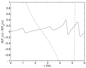
Figure 6: Indications concerning the solution of the dispersion relation $\mathcal{F}_{1}-\mathcal{F}_{2}=0$ for the Nice-like city. In the left panel: the solid and dashed curves depict $\Re(\mathcal{F}_{1})$ and $\Re(\mathcal{F}_{2})$ respectively versus frequency ($\nu$ in $Hz$) . In the right panel: the solid and dashed curves depict $\Im(\mathcal{F}_{1})$ and $\Im(\mathcal{F}_{2})$ respectively versus frequency.

Fig. 6 gives an indication of the natural frequencies of the modes of the global configuration. Recall that such a natural frequency is a solution of $\mathcal{F}_{1}-\mathcal{F}_{2}=0$, requiring that $\Re(\mathcal{F}_{1})=\Re(\mathcal{F}_{2})$, at the least. This occurs at $\nu\approx$ 2.5Hz, 5.1Hz,…. in the frequency range of the figure. The attenuation associated with a particular mode (at a frequency $\nu^{\star}$) is related to $\Im(\mathcal{F}_{1}(\nu^{\star}))-\Im(\mathcal{F}_{2}(\nu^{\star}))$.

One observes in the figure that the quasi-Love modes, which are expected to occur near 1Hz, 3Hz, 5Hz,… are either not excited or are strongly attenuated, while what appears to be the quasi-displacement free base block mode at $\nu^{QDFB}\approx 2.5$ is excited with a relatively-low attenuation. On the contrary, what appears to be the quasi stress-free base block mode at $\nu^{QDFB}\approx 5.1Hz$, is associated with a large attenuation and should therefore have little effect on the global response of the site.

The notable features of this response are that it is dominated by the quasi-displacement-free block modes, and that the influence of the periodic nature of the distribution of blocks, which manifests itself by the quasi-Cutler modes, probably appears at frequencies higher than those in the range of the figure.

9.2.3 Comparison of responses for $N_{b}=10$ and $N_{b}=\infty$

We now compare both the spectra and time histories for an infinite number of identical blocks with those of a finite number (i.e., 10) of the same blocks. The point of observation is at the center of the top segment of a block. The block under examination is the leftmost one in fig. 7, and the fifth one in fig. 8. Since the angle of incidence is 0, both the spectra and time histories of response do not change from one block to another in the $N_{b}=\infty$ structure.

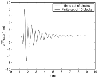
Figure 7: $2\pi$ times the spectrum (left panel) and time history (right panel) of the total displacement at the center of the top segment of a block, which is the leftmost one of a set of 10 blocks (solid curves, obtained by the FE method), or any one of an infinite set of blocks (dashed curves, obtained by the MM method ) in a Nice-like site.

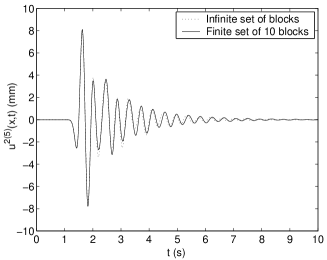
Figure 8: $2\pi$ times the spectrum (left panel) and time history (right panel) of the total displacement at the center of the top segment of a block, which is the fifth one of a set of 10 blocks (solid curves, obtained by the FE method), or any one of an infinite set of blocks (dashed curves, obtained by the MM method ) in a Nice-like site.

We note the close similarity of both the frequency and time domain responses relative to the $N_{b}=10$ and $N_{b}=\infty$ structures, even for the leftmost block of the finite configuration. This means that for a Nice-like site, the model involving an infinite number of identical blocks can used to model and/or to analyze the response phenomena in such a city.

Other than this, as concerns the response spectra, the left-most peak at $\approx 1.1$ Hz and the rightmost peak at $\approx 3.2$ Hz seem to be related to the excitation of the Haskell pseudo-modes (which is another way of saying that the corresponding quasi-Love modes are weakly excited, since these peaks would exist even if the buildings had nearly zero height). The large peak in the response spectra at $\approx 2.5$Hz is associated with the excitation of the quasi-displacement free base block mode, as expected from examination of the solutions of the dispersion relation (see fig. 6). The lengthening of the duration ($\approx$ 8 sec) of the response, with respect to the duration of the incident pulse of $\approx$ 1 sec, is mainly due to the excitation of this mode, but since the quality factor of the resonance of this mode is relatively small, the lengthening of the duration is relatively-modest. Thus, it seems that both the amplification of the amplitude, and the lengthening of duration, of seismic motion in a periodic or quasi-periodic portion of Nice, cannot take catastrophic proportions. Insofar as this conclusion concerns the amplitude of ground motion, it is in agreement with the conclusions in [32].

9.3 Finite and infinite number of blocks in a Mexico City-like site

9.3.1 Parameters

The sources of the major earthquakes in Mexico City have usually been shallow and located in the subduction zone off the Pacific coast, approximately $350km$ from Mexico City), so that modeling the solicitation of this city by a plane incident bulk wave is not realistic [18, 19]. Nevertheless, we assume such a (normally-incident) plane bulk wave solicitation, notably to enable an easy quantitative comparison between the finite and infinite city responses and qualitative comparison with previous studies [38, 10, 32, 4, 5]. The central frequency of the Ricker pulse associated with the solicitation is chosen to be $\nu_{0}=0.5Hz$.

The underground of the city is characterized by: $\rho^{0}=2000$ kg/m³, $c^{0}$=600 m/s, $Q^{0}=\infty$, $\rho^{1}=1300$ kg/m³, $c^{1}_{ref}$=60 m/s, $Q^{1}=30$, with the soft layer thickness being $h=50$ m. The Haskell frequencies are 0.3Hz, 0.9Hz, 1.5Hz,….

The blocks are 50m high, 30m in width, and their center-to-center spacing are successively chosen to be 65m, 150m and 300m. The material constants of the blocks are: $\rho^{2}=325$ Kg/m³, $c^{2}_{ref}$=100m/s, $Q^{2}=100$. The natural frequencies of the displacement-free base block modes are $\nu_{m}^{SFB}=$ 0.5Hz, 1.5Hz,…, and the quasi-Cutler mode natural frequencies (which are specific to the periodic nature of the site, with characteristic dimension $d$), are obtained from $\mathcal{F}=0$.

9.3.2 Dispersion characteristics of the modes for an infinite number of blocks

Fig. 9 gives indications concerning the solutions of the dispersion relation of the global configuration (i.e., blocks plus underground) for center-to-center spacings $d=65$m, $d=150$m and $d=300$m. For a center-to-center spacing $d=65m$, the influence of the periodic nature of the city (embodied in the parameter $d$) appears essentially at a high frequency outside the spectral bandwidth of the solicitation, while for $d=150m$ and $d=300m$, this influence can make itself felt in the spectral range of the solicitation through the quasi-Cutler modes.

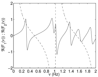
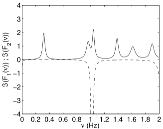
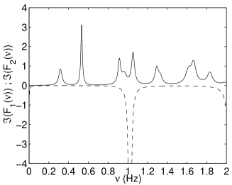
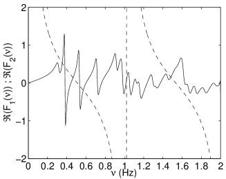
Figure 9: Indications concerning the solution of the dispersion relation $\mathcal{F}_{1}-\mathcal{F}_{2}=0$ for the Mexico City-like urban site. In the left panels: the solid and dashed curves depict $\Re(\mathcal{F}_{1})$ and $\Re(\mathcal{F}_{2})$ respectively versus frequency ($\nu$ in $Hz$) . In the right panels: the solid and dashed curves depict $\Im(\mathcal{F}_{1})$ and $\Im(\mathcal{F}_{2})$ respectively versus frequency. The top, middle and bottom panels are related to $d=65$m, $d=150$m and $d=300$m respectively.

Quasi-Love and quasi-displacement free base block modes should be excited at $\approx 0.3Hz$ and $\approx 0.5Hz$ respectively, both associated with a low attenuation. The stress-free base block mode is excited at $\approx$ 1Hz, but is highly-attenuated for all three $d$.

Quasi-Cutler modes are clearly excited with a low attenuation. In particular, for a relatively large center-to-center spacing (i.e. $d=300$), the spectral density of this type of mode is large. The fundamental quasi-Love natural frequency is probably very close to the fundamental quasi-Cutler natural frequency.

9.3.3 Seismic response for an infinite number of blocks with period $d=65$m compared to that of no blocks

Figure 10: Comparison of $2\pi$ times the spectrum (left panels) and time history (right panels) of the total displacement on the ground in absence of blocks (solid curves) with the displacement at three locations in the presence of blocks (dashed curves): i) on the ground, at a location halfway between two adjacent blocks (bottom panels), ii) at the center of the base segment of a block (middle panels), iii) at the center of the summit segment of a block (top panels).

In fig. 10 we compare the spectra and time histories in the presence and absence of the $d=65$ set of blocks.

The first resonance peak in the spectra is shifted to a lower frequency and is of higher amplitude when the blocks are present. This is the indication of the excitation of the fundamental quasi-Love mode responsible for what was termed the soil-structure interaction in the companion paper. The peak relative to the excitation of the perturbed displacement-free base block mode has a relatively high amplitude, due to both the spectrum of the incident wave and to the presence of the other blocks. Effectively, the resonance frequency does not correspond to that of the displacement-free base block mode (at which frequency the response is nil at the center of the base segment of the block), and the particular shape of the spectrum at the center of the base segment of the block is characteristic of the excitation of a multi-displacement-free base block mode and not to the excitation of a quasi displacement-free base block mode (as shown in the companion paper). This coupled mode also takes into account the so-called structure-soil-structure interaction as (see the companion paper) was suggested in sect. 7.3.

A splitting of the first peak appears in the ground (between the blocks) response. The second of the split peaks has a low quality factor, which fact means the quasi-absence of beatings in the time history of response.

The temporal displacements are of higher amplitude and duration in the presence of blocks than in the absence of blocks, particularly at the center of the top segment of the block. These results are evocative of those obtained in the companion paper for two blocks.

9.3.4 Comparison of the seismic responses for one, two and an infinite number of blocks with center-to-center separations $d=65$m

In fig. 11, we compare the spectra and time histories of response for one-block, two-block, and infinite-block configurations at the center of the top segment of one of the blocks.

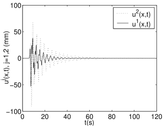
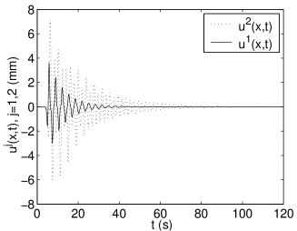
Figure 11: Comparison of $2\pi$ times the spectrum (left panels) and time history (right panels) of the total displacement on the ground in absence of blocks (solid curves) with the displacement at the center of the top segment of a $50m\times 30m$ block (dashed curves) for: i) one such blocks (top panels), ii) two such blocks with center-to-center spacing $d=65m$ (middle panels), and iii) an infinite number of such blocks with center-to-center spacing $d=65m$ (bottom panels). The one- and two-block results are taken from the companion paper and apply to the response to the wave emitted by a deep line source situated at (0m,3000m) whose amplitude, at ground level is different from that of the plane wave soliciting the infinite block structure.

This figure shows that the effect of increasing the number of blocks is essentially to increase the height of the second (i.e., higher-frequency) resonance peak at the expense of the first resonance peak, and thus to introduce stronger high-frequency oscillations in the temporal response. As the quality factor of the second resonance peak increases with $N_{b}$, the durations also increase with $N_{b}$. The combined effect of the increased quality factors and higher frequency oscillations is increased cumulative motion of the block.

In fig. 12, we compare the spectra and time histories of seismic response for one-block, two-block, and infinite-block configurations at the center of the bottom segment of one of the blocks.

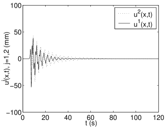
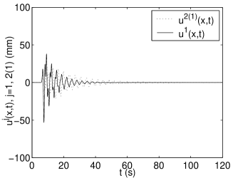
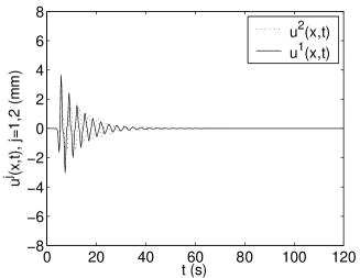
Figure 12: Comparison of $2\pi$ times the spectrum (left panels) and time history (right panels) of the total displacement on the ground in absence of blocks (solid curves) with the displacement at the center of the bottom segment of a $50m\times 30m$ block (dashed curves) for: i) one such blocks (top panels), ii) two such blocks with center-to-center spacing $d=65m$ (middle panels), and iii) an infinite number of such blocks with center-to-center spacing $d=65m$ (bottom panels). The one- and two-block results are taken from the companion paper and apply to the response to the wave emitted by a deep line source situated at (0m,3000m) whose amplitude, at ground level is different from that of the plane wave soliciting the infinite block structure.

Since the second resonance now is synonymous with a minimum of response, the aforementioned effects are not produced at the base of the block. In fact, with increasing $N_{b}$, we actually observe a decrease of the height of the first resonance peak, whose effect is to decrease the amplitude and duration of motion in the time histories.

9.3.5 Comparison of the seismic responses for ten, twenty, fourty block configurations with that of a configuration having an infinite number of blocks for center-to-center separations $d=65$m

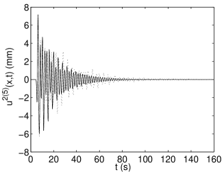
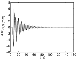
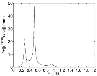
Figure 13: Comparison of $2\pi$ times the spectra (left panels) and time histories (right panels) of the total displacement at the center of the top segment of a $50m\times 30m$ block of a configuration with an infinite number of blocks (solid curves) with the displacement at the same location of a central block (dashed curves) of configurations having: i) ten such blocks (top panels), ii) twenty such blocks (middle panels), and iii) fourty such blocks. In all cases, the center-to-center spacing is $d=65m$.

In fig. 13 we compare the spectra and time histories of seismic response at the center of the top segment of a centrally-located block in configurations with 10, 20, 40 and an infinite number of $50m\times 30m$ blocks separated by $d=65$m. On the whole, these displacement responses are all the same, in both the frequency and time domains, marked by relatively-long duration duration ($\approx 2$ min), and large maximum and cumulative amplitudes. However, for the finite values of $N_{b}$, there appears some splitting of the $N_{b}=\infty$ low frequency resonance peak which gives rise to beatings in addition to those due to the presence of the two main resonance peaks.

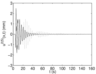
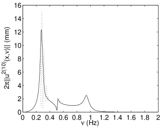
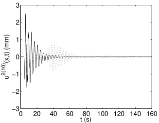
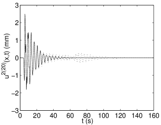
Figure 14: Comparison of $2\pi$ times the spectra (left panels) and time histories (right panels) of the total displacement at the center of the bottom segment of a $50m\times 30m$ block of a configuration with an infinite number of blocks (solid curves) with the displacement at the same location of a central block (dashed curves) of configurations having: i) ten such blocks (top panels), ii) twenty such blocks (middle panels), and iii) fourty such blocks. In all cases, the center-to-center spacing is $d=65m$.

In fig. 14 we compare the spectra and time histories of seismic response at the center of the bottom segment of a central block in configurations with 10, 20, 40 and an infinite number of $50m\times 30m$ blocks separated by $d=65$m. The splittings referred-to in the previous lines are now more apparent and give rise to more pronounced beatings, especially for the 10 and 20 block configurations. These beatings are absent for the $N_{b}=\infty$ city. The durations are quite long for the 10 and 20 block configurations, and, on the whole, the signals are evocative of what has been often observed during earthquakes in certain districts of Mexico City.

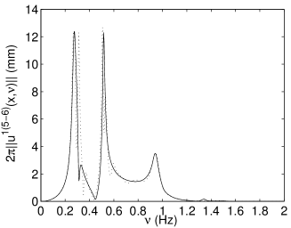
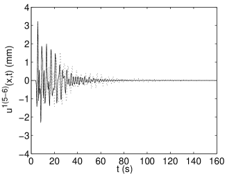
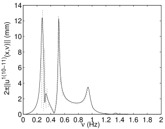
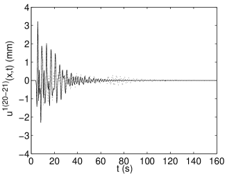
Figure 15: Comparison of $2\pi$ times the spectra (left panels) and time histories (right panels) of the total displacement at the midpoint on the ground between adjacent $50m\times 30m$ blocks of a configuration with an infinite number of blocks (solid curves) with the displacement at the same location (dashed curves) of a central region of configurations having: i) ten such blocks (top panels), ii) twenty such blocks (middle panels), and iii) fourty such blocks. In all cases, the center-to-center spacing is $d=65m$.

In fig. 15 we compare the spectra and time histories of seismic response at the midpoint on the ground between two adjacent centrally-located blocks in configurations with 10, 20, 40 and an infinite number of $50m\times 30m$ blocks separated by $d=65$m. Again, we observe two main resonance peaks for all $N_{b}$, giving rise to characteristic beatings, to which are added other beatings due to splittings of the first resonance peak, especially noticeable for finite $N_{b}$. This response is again quite evocative of ground response observed in the midst of certain districts of Mexico City during many earthquakes that have affected this city [8].

The presence of the additional low-frequency peaks in this set of figures is linked either to the (finite) number of blocks considered and/or to the total width $W$ of the finite configuration (for $N=10,~{}20,~{}40$, $W$ is equal to 650m, 1300, 2600m respectively). These peaks cannot be accounted-for in the dispersion relations written above, since they result from an analysis of configurations with an infinite number of blocks (and for which $W=\infty$).

9.3.6 Illustration of the spatial variability of response in a configuration of ten blocks for center-to-center separations $d=65$m

Fig. 16 depicts snapshots of the displacement field in the entire configuration containing ten blocks whose center-to-center distance is $d=65$m.

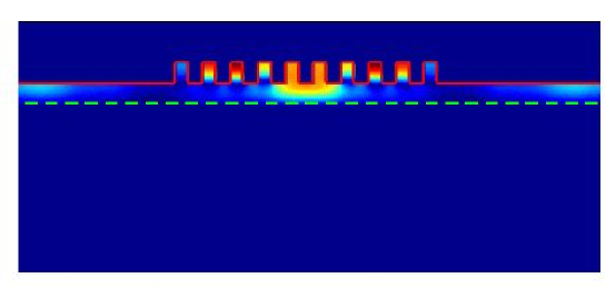
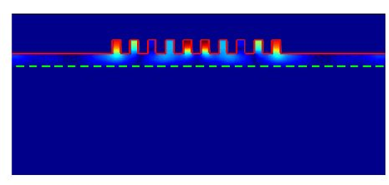
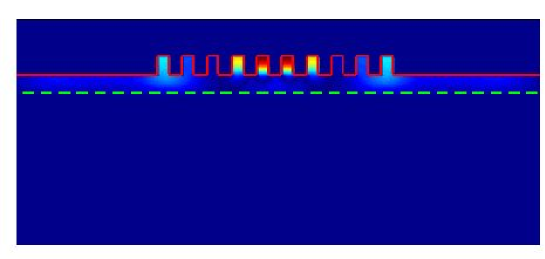
Figure 16: Snapshots at instants $t=25s$ (top panel), $t=32.5s$ (middle panel), $t=50s$ (bottom panel), of the total displacement field for $10$ identical $50m\times 30m$ blocks whose center-to-center spacing is $d=65$m.

It can be noticed that: i) the motions are still quite strong in portions of the configuration some 50s after the arrival of the initial pulse and ii) that the motion is quite variable spatially- and temporally-speaking, iii) the spatial variability extends even to within a given block.

The spatial variability of response is one of the characteristics of the motion that has often been recorded within Mexico City [14, 8].

9.3.7 Comparison of responses of the configuration without blocks to the one with $N_{b}=\infty$ blocks for $d=300$m

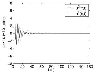
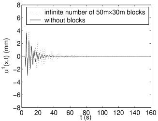
Figure 17: Comparison of $2\pi$ times the spectrum (left panels) and time history (right panels) of the total displacement on the ground in the absence of blocks (solid curves) with the displacements (dashed curves) at the center of the top segment (top panels), center of the bottom segment (middle panels) and midpoint on the ground between adjacent $50m\times 30m$ blocks, of a $N_{b}=\infty$ configuration in which $d=300$m.

In fig. 17, we compare the spectra and time histories in the presence and in the absence of the blocks. When the blocks are present, their number is infinite and their center-to-center distance is 300m.

The excitation of the multi displacement-free base block mode cannot be clearly distinguished because of the excitation of quasi-Cutler modes whose existence is related to the periodic nature of the block distribution. Note should be taken of the fact that now (i.e., for $d=300$m) these modes are visible (with a large quality factor) within the bandwidth of the solicitation, whereas they were invisible for the $d=65$m periodic structure. As previously, the soil-structure interaction appears as a resonance peak associated with the excitation of the fundamental quasi-Love mode.

These features show up at all three locations of the configuration with blocks. They manifest themselves in the time domain by: i) a larger duration (multiplied by $\approx 4$ on the top segment of the blocks with respect to its value in the absence of the blocks), ii) a larger peak amplitude (at the top of the blocks) and larger cumulative motion, and iii) pronounced beatings at all locations due to the periodic nature of the configuration.

These features are once again evocative of those which have been observed during earthquakes in certain districts Mexico City. However, the excitation of the quasi-Cutler mode, which is strongly-linked to the quasi-periodic or periodic nature of a district of the city (these districts actually exist, as seen in fig. 1), can, at best, explain only part of the features of response in this city, since the latter is not usually solicited by a (normally-incident) plane wave.

It has been shown in the companion paper, and in [18, 19] that the correct solicitation of a configuration for the study of the Michoacan earthquake (and many other earthquakes affecting Mexico City) is a cylindrical wave radiated by a shallow, laterally-distant source that gives rise to Love waves after traveling within the crust from the hypocenter to the city. In the same studies, it was shown that this type of solicitation is another cause for the large duration, large amplitude, and beatings of Mexico City response. Unfortunately, source wave solicitation cannot be treated by the quasi-modal analysis of periodic structures.

9.3.8 Comparison of the MM and FEM results for a finite set of blocks whose separation is $d=$300m

We now compare, in figs. 18, 19 and 20, the results computed by the mode-matching technique (accounting for the fundamental quasi-mode of the blocks), for an infinite number of equally-spaced identical blocks, with those we obtain by our finite-element method, for a finite number $N_{b}=10$ of equally-spaced identical blocks. In this case, $\mathbb{B}=\{1,2,...,10\}$, with the block numbers $1$ and $10$ being located at the left and right edges respectively of the finite configuration.

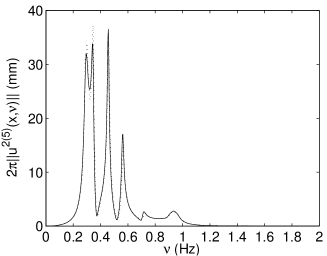
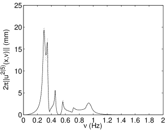
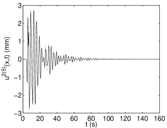
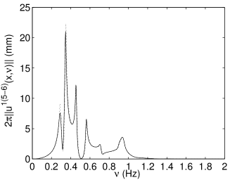
Figure 18: Comparison of $2\pi$ times the spectrum (left panels) and time history (right panels) of the total displacement as calculated by the MM method for an infinite number of $50m\times 30m$ blocks separated by $d=300m$ (solid curves) with those obtained by the FEM method in the central portion of a configuration of $10$ identical $50m\times 30m$ blocks separated by $d=300m$ (dotted curves): i) at the center of the top segment of block number 5 (top panels), ii) at the center of the base segment of block number 5, and iii) on the ground between block numbers 5 and 6.

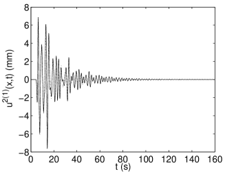
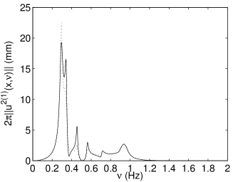
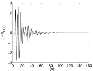
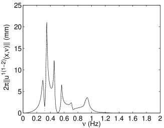
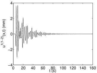
Figure 19: Comparison of $2\pi$ times the spectrum (left panels) and time history (right panels) of the total displacement as calculated by the MM method for an infinite number of $50m\times 30m$ blocks separated by $d=300m$ (solid curves) with those obtained by the FEM method in the left-hand edge portion of a configuration of $10$ identical $50m\times 30m$ blocks separated by $d=300m$ (dotted curves): i) at the center of the top segment of block number 1 (top panels), ii) at the center of the base segment of block number 1, and iii) on the ground between block numbers 1 and 2.

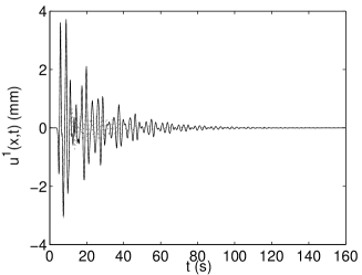
Figure 20: Comparison of $2\pi$ times the spectrum (left panels) and time history (right panels) of the total displacement as calculated by the MM method for an infinite number of $50m\times 30m$ blocks separated by $d=300m$ (solid curves) with those obtained by the FEM method in the left-hand edge portion of a configuration of $10$ identical $50m\times 30m$ blocks separated by $d=300m$ (dotted curves) at a point on the ground $150m$ to the left of the block $1$.

The width of the finite set of blocks $W$ is $3000m$ and therefore closer (than in the previous case) to the infinite width implicit in the MM theory. This may be the reason why the FE results agree quite well with the MM results within the city. The two computational modes match less well at a point on the ground outside the city (fig. 20), as one would expect.

One observes that the response is spatially variable, of long duration (attaining at some points $\approx 2$ min), with high maximum and cumulative amplitudes, and characterized by beating features, which is quite evocative of the features of many sismograms of Mexico City earthquakes [8, 14, 33, 15]. This suggests that rather largely-spaced blocks or buildings are more apt than closely-spaced blocks or buildings to induce the large-scale features (particularly the very long durations and beatings) observed in this city.

9.3.9 Illustration of the spatial variablility of response in a configuration of ten blocks separated by $d=300$m

Fig. 21 contains three snapshots, at instants $t$=25s, 32.5s and 50s, of the displacement field in the entire configuration of 10 blocks with center-to-center separation of 300m.

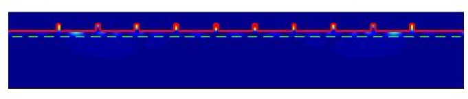
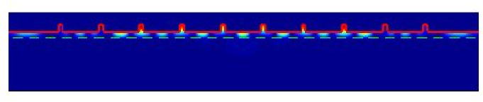
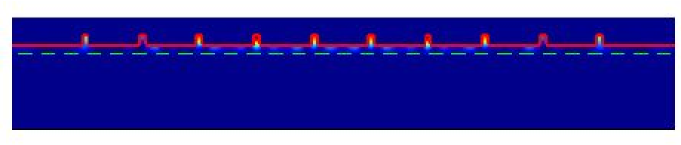
Figure 21: Snapshots at various instants, $t=25s$, $t=32.5s$, $t=50s$, of the total displacement field for $10$ identical equally-spaced $50m\times 30m$ relatively distant blocks configuration, solicited by a normal incident plane wave. The center-to-center spacing is $d=300m$.

Once again, one notes both the large- and small-scale spatio-temporal variability of response in the city site.

10 Conclusions

The response, to a plane wave initially propagating in the substratum, of a finite set of identical, equi-spaced blocks, each block modeling one, or a group of buildings, in welded contact with a soft layer overlying a hard half space, was investigated in a theoretical manner via the mode matching technique.

The capacity of this technique to account for the complex phenomena provoked by the presence of blocks on the ground was demonstrated by comparison of the numerical results to which it leads to those obtained by a finite element method.

It was shown that the presence of the blocks induces a modification of the phenomena that are produced by the configuration without blocks, or of a configuration of closed blocks disconnected from the geophysical half-space. In particular, the blocks modify the dispersion relation of what, in the absence of the blocks, constitutes the Love modes. Moreover, the periodic nature of the urban site is responsible for the existence of another vibrational mode which is a variant of the Cutler mode encountered in electromagnetic waveguide structures.

The dispersion relation for the periodic configurations with an infinite number of blocks is very complex, but an approximation of this relation lends itself to a fairly-explicit theoretical analysis, inspired notably by the method first adopted in the electromagnetic wave community. The general features of this dispersion relation, revealed by the theoretical analysis (and manifested by the existence of several types of vibrational modes), were shown to actually exist by means of the numerical study.

The excitation of the vibrational modes was then studied in the particular case of city districts with 10 and an infinite number of identical, periodically-disposed blocks. A common feature of the influence of the blocks is the excitation of the quasi-Love mode, which occurs even for solicitation by a plane wave (recall that, for this type of solicitation, it is not possible to excite ordinary Love modes in a flat ground (i.e., no blocks)/soft horizontal layer/hard substratum configuration [18]). The trace of quasi-Love mode excitation in the frequency domain was shown to be a shift to lower frequency and an increase of the amplitude of the first (lowest-frequency) peak of the response.

The change of the phenomena provoked by plane wave solicitation, from a configuration without blocks (for which there exist only bulk waves in the geophysical structure), to one with blocks (for which there exist quasi-Love modes characterized by a field in the substratum that is predominantly a surface wave in the substratum) is a manifestation of the so-called soil-structure interaction.

Multi displacement-free base block modes were shown to be excited in all the configurations and to correspond to a coupled mode.

The modifications of the response due to the presence of blocks separated by 65m were found to be rather modest in the Nice-like site.

The modifications of the frequency-domain response (and less so of the time-domain response) were found to be fairly substantial for structures involving blocks separated by 65m in the Mexico City-like site. In particular, 10 or 20 blocks separated by 65m, were shown to give rise to anomalous features (amplifications of peak and cumulative motion, large durations and beatings) that are even closer to those observed in Mexico City than configurations with a larger number (40, $\infty$) of blocks.

All the anomalous features found for the Mexico City-like site with 10 or an infinite number of blocks were found to be closer to the actually-observed anomalous features observed during earthquakes in Mexico City when the separation between blocks is 300m rather than 65m. This was found to be due to the fact that the structure with the larger period enables the quasi-Cutler mode to make itself felt within the range of frequencies of the source.

The theoretical findings and numerical results of the present study cannot account for all the anomalous phenomena observed in many of the earthquakes in Mexico City (notably the exceptionally-long durations) for the obvious reasons that the model adopted herein, i.e., SH plane wave solicitation, 2D, periodic geometries, simple underground (horizontal homogeneous soft layer of infinite lateral extent overlying a homogeneous lossless hard substratum), simple homogenized building blocks, linear soil behavior, etc., is incomplete, and in some respects, rather far removed from reality. Nevertheless, the results of our study indicate that it is possible that the excitation of vibrational modes, whose structure is closely-related to those described herein, was responsible for at least part of the large-scale, anomalous mechanical effects that have caused so much damage in past earthquakes in urban areas.

The most important finding of this work, which substantiates those obtained in [38, 34, 17], is that the presence of groups of buildings (i.e., city blocks) can modify substantially the seismic motion in a city. Moreover, provided the blocks are arranged quasi-periodically with a sufficiently large period $d$, the seismic motion is of longer duration, and of higher cumulative (sometimes peak) amplitude on the ground (and, of course, in the buildings) than when the built structures are not present.

Therefore, it is advisable to integrate (as is starting to be done [13]) the presence, composition and layout, of buildings, together with, and to the same extent as, the features of the underground structure and composition, into the large-scale computer codes that are being employed [35] to predict the level and durations of shaking in highly-populated, economically-important, earthquake-prone areas.

References

- [1] Auld, B.A., Gagnepain, J.J. and Tan, 1976, Horizontal shear surface waves on corrugated surfaces, Elecrton.Lett.,12, 650-651.
- [2] Bécache, E., Joly, P. and Tsogka, C., 2001, Fictitious domains, mixed finite elements and perfectly matched layers for 2D elastic wave propagation, J.Comput.Acoust., 9, 1175-1203.
- [3] Borgnis C.H. and Papas C.H., 1958, Electromagnetic waveguides and resonators, in Handbuch der Physik, vol.16, Flügge (ed.), Springer, Berlin, 378-384.
- [4] Boutin C. and Roussillon P., 2004, Assessement of the urbanisation effect on seismic response, Bull.Seism.Soc.Am., 94, 252-268.
- [5] Boutin C. and Roussillon P., 2006, Wave propagation in presence of oscillators on the free surface, Int.J.Engrg.Sci., 44, 180-204.
- [6] Cardenas-Soto M. and Chavez-Garcia F.J., 2003, Regional path effect on seismic wave propagation in central Mexico, Bull.Seism.Soc.Am., 93, 973-985.
- [7] Cardenas-Soto M. and Chavez-Garcia F.J., 2006, Seismic wavefield analysis in Mexico City using accelerometric arrays, Abstracts of the First European Conference on Earthquake Engineering and Seismology, SSS, Geneva, 166.
- [8] Chavez-Garcia F.J. and Bard P.Y., 1994, Site effects in Mexico-city height years after the september 1985 Michoacan earthquakes, SoilDyn.Earthq.Engrg., 13, 229-247.
- [9] Chavez-Garcia F.J. and Salazar L., 2002, Strong motion in central Mexico: a model on data analysis and simpler modeling, Bull.Seism.Soc.Am., 92, 3087-3101.
- [10] Clouteau D. and Aubry D., 2001, Modifications of the ground motion in dense urban areas, J.Comput.Acoust., 9, 1-17.
- [11] Cutler C.C., 1944, Electromagnetic waves guided by corrugated structures, Bell Telephone Lab. Technical Report MM44-160-218.
- [12] Collino, F. and Tsogka, C., 2001, Application of the PML absorbing layer model to the linear elastodynamic problem in anisotropic heterogeneous media, Geophys., 66, 294-305,
- [13] Fernandez-Ares A. and Bielak J., 2006, Urban seismology: interaction between earthquake ground motion and multiple buildings in urban regions, in ESG 2006, Bard P.-Y., Chaljub E., Cornu C., Cotton F. & Guéguen P. (eds.), LCPC, Paris, 87-96.
- [14] Flores J., Novaro O. and Seligman T.H., 1987, Possible resonance effect in the distribution of earthquake damage in Mexico City, Nature, 326.
- [15] Furumura T. and Kennett B.L.N., 1998, On the nature of regional seismic phase-III. The influence of crustal heterogénéity on the wavefield for subduction earthquakes: the 1989 Michoacan, and 1995 Copala, Guerrero, Mexico earthquakes, Geophys.J.Intl., 135, 1060-1085.
- [16] Groby, J.P. and Tsogka, C., 2006, A time domain method for modeling viscoacoustic wave propagation, J.Comput.Acoust., 14, 201-236.
- [17] Groby J.P., Tsogka C. and Wirgin A., 2005, Simulation of seismic response in a city-like environment, Soil Dyn.Earthq.Engrg., 25, 487-504
- [18] Groby J.P. and Wirgin A., 2005, 2D ground motion at a soft viscoelastic layer/hard substratum site in response to SH cylindrical sesimic waves radiated by deep and shallow line sources I. Theory, Geophys.J.Intl., 163, 165-191.
- [19] Groby J.P. and Wirgin A., 2005, 2D ground motion at a soft viscoelastic layer/hard substratum site in response to SH cylindrical sesimic waves radiated by deep and shallow line sources II. Numerical Results, Geophys.J.Intl., 163, 192-224.
- [20] Gueguen P., Bard P.-Y. and Chavez-Garcia F.J., 2002, Site-city seismic interaction in Mexico City like environments : an analytic study, Bull.Seism.Soc.Am., 92, 794-804.
- [21] Gulyaev Y.V. and Plesskii V.P., 1978, Slow, shear surface acoustic waves in a slow-wave structure on a solid surface, Sov.Phys.Tech.Phys., 23, 266-269.
- [22] Haghshenas E., Jafari M., Bard P.-Y., Moradi A.S. and Hatzfeld D., 2006, Preliminary results of site effects assessment in the city of Tabriz (Iran) using earthquakes recording, in ESG 2006, Bard P.-Y., Chaljub E., Cornu C., Cotton F. & Guéguen P. (eds.), LCPC, Paris, 993-1001.
- [23] Hougardy R.W. and Hansen R.C., 1958, Oblique surface waves over a corrugated conductor, IRE Trans.Anten.Prop., AP-6, 370-376.
- [24] Hurd R.A., 1954, The propagation of an electromagnetic wave along an infinite corrugated surface, Canad.J.Phys., 32, 727-734.
- [25] Iwata T., Kagawa T. Petukhin A. and Onishi Y., 2006, Basin and crustal structure model for strong ground motion simulation in Kinki, Japan, in ESG 2006, Bard P.-Y., Chaljub E., Cornu C., Cotton F. & Guéguen P. (eds.), LCPC, Paris, 435-442.
- [26] Kjartansson E., 1979, Constant Q wave propagation and attenuation, J.Geophys.Res., 84,4737-4748.
- [27] Maeda N., Nakajima Y., Matsuda I. and Abeki N., 2006, Evaluation of seismic amplification characteristics at a university campus with complicated relief of basement, in ESG 2006, Bard P.-Y., Chaljub E., Cornu C., Cotton F. & Guéguen P. (eds.), LCPC, Paris, 443-451.
- [28] Mateos J.L., Flores J., Novaro O., Seilgman T.H. and Alvarez-Costado J.M., 1993, Resonant response models for the valleys of Mexico - II The trapping of horizontal P waves, Geophys.J.Intl.,113, 449-462.
- [29] Morse P.M. and Feshbach H., 1953, Methods of Theoretical Physics, Mc Graw-Hill, New York, 1953.
- [30] Perez-Rocha L.E., Sanchez-Sesma F.J. and Reinoso E., 1991, Three-dimensional site effects in Mexico-city: evidence from the accelerometric network observation and theorical results, In Proc. 4th Intl. Conf. on Seismic Zonation, volume II, 327-334.
- [31] Rotman W., 1951, A study of single surface corrugated guides, Proc. IRE, 39, 952-959.
- [32] Semblat J.F., Guégen P., Kham M., Bard P.Y. and Duval A.M., 2003, Site-city interaction at local and global scales, In Proc. 12th European Conf. on Earthq.Engrg., paper no. 807.
- [33] Singh S.K. and Ordaz M., 1993, On the origin of long coda observed in the lake-bed strong-motion records of Mexico City, Bull.Seism.Soc.Am., 83, 1298-1306.
- [34] Tsogka C. and Wirgin A., 2003, Simulation of seismic response in an idealized city, Soil Dynam.Earthquake Engrg., 23, 391-402.
- [35] Wald D.J. and Graves R.W., 1998, The seismic response of the Los Angeles Basin, California, Bull.Seism.Soc.Am., 88, 337-356.
- [36] Wirgin A., 1988, Love waves in a slab with rough boundaries, in Recent Developments in Surface Acoustic Waves, Parker D.F. and Maugin G.A. (eds.), Springer series on wave phenomena, Berlin, 145-155.
- [37] Wirgin, A., 1995, Resonant response of a soft semi-circular cylindrical basin to an SH seismic wave, Bull.Seism.Soc.Am., 85, 285-299.
- [38] Wirgin A. and Bard P.-Y., 1996, Effects of buildings on the duration and amplitude of ground motion in Mexico City, Bull.Seism.Soc.Am., 86, 914-920.