Infectious Default Model with Recovery and Continuous Limits

Abstract

We introduce an infectious default and recovery model for $N$ obligors. The obligors are assumed to be exchangeable and their states are described by $N$ Bernoulli-type random variables $S_{i}(i=1,\cdots,N)$. They are expressed by multiplying independent Bernoulli variables $X_{i},Y_{ij}$ and $Y^{\prime}_{ij}$, and the default and recovery infections are described by $Y_{ij}$ and $Y^{\prime}_{ij}$. We obtain the default probability function $P(k)$ for $k$ defaults. By considering a continuous limit, we find two nontrivial probability distributions with a reflection symmetry of $S_{i}\leftrightarrow 1-S_{i}$. Their profiles are singular and oscillating and we theoretically investigate it. We also compare $P(k)$ with an implied default distribution function inferred from the quotes of iTraxx-CJ, which is a portfolio credit derivative of Japanese 50 companies. In order to explain the behavior of the implied distribution, the recovery effect may be necessary.

1 Introduction

The cooperative phenomena, especially phase transitions, have been extensively studied and continue to be important subjects until today. They have provided universal paradigm for physics, sociology, and economy. The economical systems composed of a large number of interacting units have been studied from this viewpoint. [1, 2] Recently, systemic failure problems are being focused upon in econophysics, [3, 4, 5, 6, 7] financial engineering, [8, 9, 10, 11, 12] and computer engineering, [13] and many probabilistic models have been proposed. This has been motivated by the fact that the description of systemic failures is necessary to control and manage them. Another motivation is that credit risk markets are now growing, and the pricing of products is an immediate concern.[14] For this purpose, it is necessary to develop probabilistic models that can describe credit risks.

The difficulty in the description of systemic failures arises from the fact that they are not independent events. If they are independent, the description is very easy and we only need Bernoulli-type random variables $S_{i}$ denoting the element $i$’s failure or not by $S_{i}=1$ or $S_{i}=0$ respectively. However, there are many phenomena wherein the “correlation” between the failure events is very important. For example, in a network of storage systems, if a node fails, the failure can propagate to other nodes.

In credit risk markets, the same type of risk propagation is found to occur. A percolation-type probabilistic model was proposed to describe bank bankruptcies, where interbank deposits lead to collective credit risks. The probability of $l$ failures obeyed the power law $P(l)\sim l^{1-\tau}$ with the Fisher exponent $\tau$ at its critical point. In a study,[8] a default infection mechanism was proposed to describe the risk-dependency structures. The constituents are obligors, and the risk is whether he (or she) can refund before the expiry date. Such a risk is called a default risk. Davis and Lo introduced independent Bernoulli-type random variables $Y_{ij}$, which describes the infection from a bad obligor $j$ to a good one $i$. They explicitly obtained the probability function for $k$ defaults, $P(k)$. They estimated the effect of the default correlation on $P(k)$.

One of the crucial problems with these studies is that their it is difficult to describe whether $P(k)$ values do describe the empirical default distribution $P(k)$ or not. Because of the relative scarcity of good data on credit events, it was impossible to compare the models by using the empirical data. Recently, from the market quotes on credit risk products, it becomes possible to infer the default distribution function.[12, 15] We can compare and calibrate the probabilistic models. In the present paper, we generalize the model proposed by Davis and Lo by introducing a recovery effect. We compare the default distribution $P(k)$ with an implied value of that of the credit market and calibrate the model parameters. With regard to the bulk shape, we see that the calibrated $P(k)$ value looks similar.

The outline of the present paper is as follows. Section 2 gives a brief introduction to the infectious default model proposed by Davis and Lo,[8] and we modify it by introducing a recovery process. We obtain the default probability function $P(k)$ for $k$ defaults. In section 3, we take the continuous limit of $P(k)$ with finite $P_{d}$ and non zero correlation $\rho>0$. We find two non trivial probability distribution functions with a reflection symmetry. They exhibit oscillating behaviors and we investigate the mechanism. We compare the model distribution function $P(k)$ with the market implied function in section 4. Section 5 summarizes our results and future problems are discussed.

2 Infectious default model

We consider $N$ exchangeable obligors whose states are described by random variables $S_{i}(i=1,2,\cdots,N)$ such that $S_{i}=1$ if obligor $i$ defaults and $S_{i}=0$ otherwise. Here, the term “exchangeable” means the non-dependency of the joint probabilities $P(S_{1},S_{2},\cdots,S_{N})$ on the exchange of $S_{i}\leftrightarrow S_{j}$ for any pair of $(i,j)$. The number of defaults is

$$K=S_{1}+S_{2}+\cdots+S_{N}.$$ (1)

The value of $S_{i}$ is determined as follows. For $i=1,\cdots,N$ and $j=1,\cdots,N$ with $j\neq i$, let $X_{i},Y_{ij}$ be independent Bernoulli-type random variables with probability function

$$\mbox{Prob.}[X_{i}=1] = p,$$

$$\mbox{Prob.}[Y_{ij}=1] = q.$$ (2)

$S_{i}$ are defined as

$$S_{i}=X_{i}+(1-X_{i})(1-\Pi_{j\neq i}(1-Y_{ij}X_{j})).$$ (3)

Here, $X_{i}$ is the internal state variable which describes whether the obligor is in a good state ($X_{i}=0$) or not ($X_{i}=1$). $S_{i}$ is also the state variable that describes whether the obligor is defaulted ($S_{i}=1$) or not ($S_{i}=0$), this is determined by not only the internal state but also the external environment. If $X_{i}=1$, $S_{i}=1$ and the obligor is defaulted. Even if $X_{i}=0$, obligor $i$ can be defaulted. $Y_{ij}$ represents the influence of another bad obligor ($X_{j}=1$) on obligor $i$. A default infection from a bad obligor $j$ takes place if $Y_{ij}=1$ and $X_{j}=1$. $S_{i}$ becomes 1 and the obligor is defaulted. The second term of eq.(3) represents this effect.

We introduce a supporting effect from other good obligors in addition to the default infection. In fact, it may occur that a good obligor supports other bad obligors and the latter can circumvent their defaults. We introduce new independent Bernoulli-type random variables $Y^{\prime}_{ij}$ in addition to eq.(2). For $i=1,\cdots,N$ and $j=1,\cdots,N$ with $j\neq i$, they have the probability function

$$\mbox{Prob.}[Y_{ij}^{\prime}=1]=q^{\prime}.$$ (4)

We introduce the following model equation for $S_{i}$:

$$S_{i}=X_{i}\Pi_{j\neq i}(1-Y_{ij}^{\prime}(1-X_{j}))+(1-X_{i})(1-\Pi_{j\neq i}(1-Y_{ij}X_{j})).$$ (5)

Eq.(5) reveals that even when $X_{i}=1$, if $X_{j}=0$ and $Y^{\prime}_{ij}=1$, obligor $i$ is supported by obligor $j$ and avoids being defaulted. We note that eq.(5) has a default, non-default symmetry. We get $1-S_{i}$ by substituting $X_{i}\to 1-X_{i}$ and $Y_{ij}\leftrightarrow Y^{\prime}_{ij}$. This model can be reduced to the original infectious default model by substituting $Y^{\prime}_{ij}=0$ into eq.(5).

The probability distribution function $P(k)$ for $k$ defaults is given by

$$P(k)=\mbox{Prob.}[K=k]={{}_{N}C_{k}}\times\sum_{l=0}^{k}\sum_{m=0}^{N-k}\alpha_{N,k}^{p,q,q^{\prime}}(l,m)$$ (6)

where

$$\alpha_{N,k}^{p,q,q^{\prime}}(l,m) = {}_{k}C_{l}\times{{}_{N-k}C_{m}}\times p^{N-k-m+l}(1-p)^{k-l+m}$$ (7)

$$\ \ \times(1-q^{\prime})^{l(k+m-l)}(1-q)^{m(N-k-m+l)}$$

$$\ \ \times(1-(1-q)^{N-k-m+l})^{k-l}(1-(1-q^{\prime})^{k+m-l})^{N-(k+m)}.$$

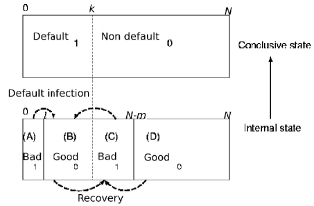
Figure 1: Pictorial representation from internal states $\{X_{i}\}$ to a conclusive state of $k$ defaults and $N-k$ non-defaults.

We explain the derivation of eq.(7). In Fig.1, there are $N$ obligors. $k$ obligors are defaulted and $N-k$ obligors are non-defaulted. The $k$ defaulted obligors are classified into two categories: (A) and (B). (A) contains $l$ bad obligors, which are never supported by other good obligors. (B) contains $k-l$ good obligors, which are infected by other bad obligors and thus get defaulted. The number of different possible combinations of $l$ items from $k$ different items is ${}_{k}C_{l}$. Further, there are two categories (C) and (D) for the $N-k$ non-defaulted obligors. (C) contains $N-k-m$ bad obligors and (D) contains $m$ good obligors. The $N-k-m$ bad obligors are supported by other good obligors and they are prevented from being defaulted. The $m$ good obligors are never infected to be defaulted. The number of different possible combinations of $m$ items from $N-k$ different items is ${}_{N-k}C_{m}$. In other words, the conclusive $k$ defaults and $N-k$ non-defaults are made from the $N-k-m+l$ bad obligors and $k-l+m$ good obligors in the internal configuration by the infection and recovery mechanism. The internal configuration is realized with probability $p^{N-k-m+l}(1-p)^{k-l+m}$. $l$ bad obligors among the $N-k-m+l$ obligors are not supported by the $k-l+m$ good obligors; this probability is given by $(1-q^{\prime})^{(k-l+m)l}$. $m$ good obligors are never infected by $N-k-m+l$ bad obligors; this probability is given by $(1-q)^{m(N-k-m+l)}$. $k-l$ good obligors must be infected by $N-k-m+l$ bad obligors; this probability is given by $(1-(1-q)^{N-k-m+l})^{k-l}$. $N-k-m$ bad obligors must be supported by $k-l+m$ good obligors; this probability is given by $(1-(1-q^{\prime})^{k+m-l})^{N-k-m}$. Therefore, the probability of $k$ defaults and $N-k$ non-defaults from a configuration $(l,m)$ is given by $\alpha_{N,k}^{p,q,q^{\prime}}(l,m)$, as shown in eq.(7). We obtain $P(k)$ as the summation of $\alpha_{N,k}^{p,q,q^{\prime}}(l,m)$ over $l,m$.

The expected value of the number of defaults $K$ is

$$<K>=N[p(1-q^{\prime}(1-p))^{N-1}+(1-p)(1-(1-qp)^{N-1})],$$ (8)

and the default probability $P_{d}$ is given as

$$P_{d}=<K>/N=p(1-q^{\prime}(1-p))^{N-1}+(1-p)(1-(1-qp)^{N-1}).$$ (9)

The variance is

$$\sigma^{2}_{K}=<K>+N(N-1)\beta_{N}^{p,q,q^{\prime}}-<K>^{2},$$ (10)

where

$$\beta_{N}^{p,q,q^{\prime}} = <S_{i}S_{j}>$$ (11)

$$= p^{2}\{1-2q^{\prime}(1-p)+q^{\prime 2}(1-p)^{2}\}^{N-2}$$

$$\ \ +2p(1-p)(1-q^{\prime})\{(1-q^{\prime}(1-p))^{N-2}$$

$$\hskip 28.45274pt-(1-q)(1-q^{\prime}(1-p)-pq)^{N-2}\}$$

$$\ \ +(1-p)^{2}[1-2(1-pq)^{N-2}+(1-2pq+pq^{2})^{N-2}]$$

and the correlation coefficient is given by

$$\rho=\frac{\beta_{N}^{p,q,q^{\prime}}-P_{d}^{2}}{P_{d}(1-P_{d})}.$$ (12)

We find that there are multiple solutions $(p,q,q^{\prime})$ corresponding to a value of $P_{d}$. In particular, for large $N$, there are three solutions. For example, there are three solutions $p=0.808310,0.5$, and $0.191680$ for $N=100,P_{d}=0.5$, and $q=q^{\prime}=0.05$. On the other hand, there is only one solution $p=0.5$ for $N=50,P_{d}=0.5$, and $q=q^{\prime}=0.05$. This is because for arbitrary $q,q^{\prime}\neq 0$, $P_{d}$ behaves as that in Fig.3. $P_{d}(p,q,q^{\prime})$ starts from 0 at $p=0$ to 1 at $p=1$. For intermediate values of $p$, $P_{d}$ rapidly increases to 1 and then decreases to 0 near $p=1$ in the large $N$ limit. Thereafter, $P_{d}$ again increase rapidly to 1 toward $p=1$. Such a behavior can be explained by eq.(9). There are three $p$ solutions corresponding to a $P_{d}$ value; they are referred to as left, middle and right solutions according to the order of $p$. The parameter region $(q,q^{\prime})$ in which there are three solutions of $p$ expands with $N$; further, for the limit $N\to\infty$, it covers the entire parameter space $(q>0,q^{\prime}>0)$.

The profiles of the three solutions are shown in Fig.3. We set $N=50,P_{d}=0.5$, and $q=q^{\prime}=0.2$. The three solutions are realized at $p=0.079281$ (left), $p=0.5$ (middle), and $p=0.920719$ (right). The profiles of the probability distribution functions of the left and right solutions are reflection symmetric. The origin of the symmetry arises from the reflection symmetry of eq.(5). $P(k)$ for the middle solution ($p=0.5$) has a symmetrical profile and is almost a binomial distribution $\mbox{Bi}(50,0.5)$.

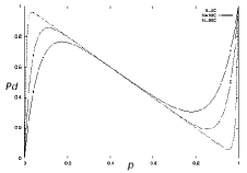
Figure 2: Plot of $P_{d}$ vs. $p$. We set $N=50,100$, and $500$, $q=0.3$, and $q^{\prime}=0.2$.

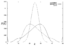
Figure 3: Plot of $P(k)$ for $P_{d}=0.5$ and $q=q^{\prime}=0.2$. The left, middle, and right solutions are plotted.

3 Continuous limit and probability distribution function

In this section, we consider the continuous limit of eq.(7). It is required to take the limit $N\to\infty$ with non zero correlation because the probability distribution function of the uncorrelated variables is a binomial distribution. Its continuous limit reduces to a trivial delta function. We need to consider the continuous limit with fixed $P_{d}$ and $\rho$. Writing explicitly, $\rho=(<S_{i}S_{j}>-<S_{i}><S_{j}>)/P_{d}(1-P_{d})$ is calculated as

$$\rho = \{p^{2}[(1+(q^{\prime 2}-2q^{\prime})(1-p))^{N-2}-(1-2q^{\prime}(1-p)+q^{\prime 2}(1-p)^{2})^{N-1}]$$ (13)

$$\ \ +(1-p)^{2}[(1+(q^{2}-2q)p)^{N-2}-(1-2qp+q^{2}p^{2})^{N-1}]$$

$$\ \ -2p(1-p)[(1-p)q(1-pq)^{N-2}-pq^{\prime}(1-q^{\prime}(1-p))^{N-2}$$

$$\ \ \ \ \ +(1-q^{\prime})(1-q)(1-qp-q^{\prime}(1-p))^{N-2}$$

$$\ \ \ \ \ -(1-q^{\prime}(1-p))^{N-1}(1-qp)^{N-1}]\}/P_{d}(1-P_{d}),$$

where

$$P_{d}=p(1-q^{\prime}(1-p))^{N-1}+(1-p)(1-(1-qp)^{N-1}).$$ (14)

There are three terms in eq.(13). The first term is derived from $<X_{i}X_{j}>$, which is proportional to $p^{2}$. The second term is derived from $<(1-X_{i})(1-X_{j})>$, which is proportional to $(1-p)^{2}$. The last term is derived from $<X_{i}(1-X_{j})>$ and $<(1-X_{i})X_{j}>$, which is proportional to $2p(1-p)$. At least one term must be non-zero in the continuous limit in order to retain the correlation. In order to fix $P_{d}$ in the limit $N\to\infty$, it is necessary to set the parameters $p\times q$ or $(1-p)\times q^{\prime}$ to be proportional to $1/N$ due to the presence of the $N$th power in eq.(14). To satisfy this condition, we must set $p,q,q^{\prime}$ such that the non zero correlation is maintained. Using a proportional coefficient $\alpha$, if we set $p=\alpha/N$, the resulting expression corresponds to the left solution in the previous section. The correlation is maintained due to the first term of eq.(13). For $p=1-\alpha/N$, the resulting expression corresponds to the right solution; the second term of eq.(13) remains. Instead, if we set $q,q^{\prime}\propto 1/N$ and $p$ to be finite, eq.(13) vanishes in the limit $N\to\infty$ and the correlation disappears. The resulting expression corresponds to the middle solution in the previous section and the model becomes a binomial distribution.

In the above limit, $P_{d}$ and $\rho$ can be easily estimated. We set $p=\alpha/N$ and substitute this value in eq.(13) and eq.(14). We obtain

$$P_{d}=1-e^{-\alpha q},$$ (15)

$$\rho=\frac{e^{-\alpha q}(e^{\alpha q^{2}}-1)}{1-e^{-\alpha q}}.$$ (16)

If we set $p=1-\alpha/N$, we get

$$P_{d}=e^{-\alpha q^{\prime}}$$ (17)

and

$$\rho=\frac{e^{-\alpha q^{\prime}}(e^{\alpha q^{\prime 2}}-1)}{1-e^{-\alpha q^{\prime}}}.$$ (18)

We see that the above two non trivial solutions can retain their non-zero correlations in the continuous limit. From the symmetric property of the model, we note that eq.(17) and eq.(18) can be derived by the substituting $P_{d}\leftrightarrow 1-P_{d},q\leftrightarrow q^{\prime}$, and $p\leftrightarrow 1-p$ in eq.(15) and eq.(16).

We show the profiles of the probability distributions $P(k)$ with $p=\alpha/N$ and $p=1-\alpha/N$ in Fig.5 and Fig.5. They show reflection symmetric profiles ($k\leftrightarrow N-k$)and have very singular oscillating shapes. Hereafter, we interpret the oscillating behavior based on eq.(7).

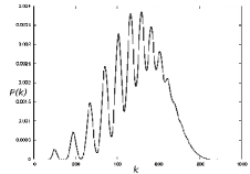
Figure 4: Plot of $P(k)$ for $P_{d}=0.5,q=q^{\prime}=0.1,N=1000,\\ p=\alpha/N=0.007$, and $\rho=0.071773$

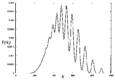
Figure 5: Plot of $P(k)$ for $P_{d}=0.5,q=q^{\prime}=0.1,N=1000,\\ p=1-\alpha/N=0.993$, and$\rho=0.071773$

The behavior of $P(k)$ can be understood by considering each term in eq.(6). It is expressed as a summation of $\alpha^{p,q,q^{\prime}}_{N,k}(l,m)$. The difference between $P(k)$ for $p=\alpha/N$ and $p=1-\alpha/N$ is only observed in the first part of eq.(7), $p^{N-k-m+l}(1-p)^{k-l+m}$. For $p=\alpha/N$,

$$p^{N-k-m+l}(1-p)^{k-l+m}=\Big{(}\frac{\alpha}{N}\Big{)}^{N-k-m+l}\Big{(}1-\frac{\alpha}{N}\Big{)}^{k-l+m}.$$ (19)

This suggests that $\alpha_{N,k}^{p,q,q^{\prime}}(l,m)$, which contributes significantly to $P(k)$, should satisfy the condition $k+m-l\approx N$. From the second line of eq.(7), $(1-q^{\prime})^{l(k+m-l)}(1-q)^{m(N-k-m+l)}$, we see that $l$ should be equal to 0 because $k-l+m\approx N$. Therefore, $\alpha_{N,k}^{p,q,q^{\prime}}$ with $l=0$ and $m\approx N-k$ significantly contributes to $P(k)$. The third part of eq.(7), $(1-(1-q)^{N-k-m+l})^{k-l}(1-(1-q^{\prime})^{k+m-l})^{N-k-m}$, has non zero value with the above condition in the limit $N\to\infty$.

We set $l=0$ and $m=N-k-n\hskip 2.84544pt(n/N\ll 1)$ in eq.(7). The probability distribution function can be expressed as

$$\lim_{N\to\infty}P_{p=\alpha/N}(k)\approx_{N}C_{k}\times\sum_{n\ll N}\alpha_{N,k}^{p=\alpha/N,q,q^{\prime}}(l=0,m=N-k-n),$$ (20)

where

$$\alpha_{N,k}^{p=\alpha/N,q,q^{\prime}}(l=0,m=N-k-n) = {}_{N}C_{k}\times_{N-k}C_{N-k-n}\Big{(}\frac{\alpha}{N}\Big{)}^{n}\Big{(}1-\frac{\alpha}{N}\Big{)}^{N-n}$$ (21)

$$\ \ \times(1-q)^{(N-k-n)n}(1-(1-q)^{n})^{k}.$$

Instead of $k$, we use a normalized variable $x\equiv\frac{k}{N}$ and express $\alpha_{x}^{\alpha,q,q^{\prime}}(n)=\alpha_{N,k}^{p=\alpha/N,q,q^{\prime}}(l=0,m=N-Nx-n)$. The function ${}_{N}C_{Nx}\cdot\alpha_{x}^{\alpha,q,q^{\prime}}(n)$ has a very narrow profile, and the position of the peak $x_{n}$ is given by the condition $\partial{}_{N}C_{Nx}\cdot\alpha_{x}^{\alpha,q,q^{\prime}}(n)/\partial x=0$ at $x=x_{n}$. We get

$$x_{n}(1-q)^{n}=(1-x_{n}-\frac{n}{N})(1-(1-q)^{n}).$$ (22)

In the limit $N\to\infty$, we obtain the probability density function $p(x)$ as follows.

$$p(x)=\sum_{n=0}\frac{\alpha^{n}e^{-\alpha}}{n!\sqrt{2\pi\sigma_{n}^{2}}}\exp\Big{(}-\frac{(x-x_{n})^{2}}{2\sigma_{n}^{2}}\Big{)},$$ (23)

where

$$x_{n} = 1-(1-q)^{n},$$ (24)

$$\sigma_{n}^{2} = \frac{1}{N}(1-q)^{n}(1-(1-q)^{n}).$$ (25)

$p(x)$ can be expressed as

$$p(x) = \sum_{n=0}p(x\mid n)P_{ini}(n),$$ (26)

$$p(x\mid n) = \frac{1}{\sqrt{2\pi\sigma_{n}^{2}}}\exp\Big{(}-\frac{(x-x(n))^{2}}{2\sigma_{n}^{2}}\Big{)},$$ (27)

$$P_{ini}(n) = \frac{\alpha^{n}e^{-\alpha}}{n!}.$$ (28)

$P_{ini}(n)$ is the probability of the occurrence of $n$ internal bad obligors and it is a Poisson probability function. $p(x\mid n)$ is the resulting probability density after $n$ bad companies appear and infections occur from them. By the decomposition of eq.(26), it is easy to understand the oscillating behavior of $p(x)$. In Fig.6, $p(x)$ is clearly decomposed into the product of the normal distribution $p(x\mid n)$ and $P_{ini}(n)$.

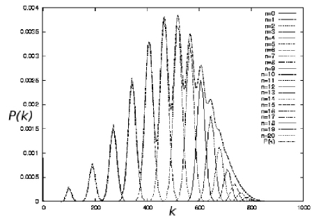
Figure 6: Plot of $P(k)$ of the left solution in Fig.5 and the plot of the normal distribution $p(x\mid n)P_{ini}(n)$ for $0\leq n\leq 20$.

We comment on De Finetti’s theorem, which states that the joint probability function of $N$ exchangeable Bernoulli-type variables can be expressed as a mixture of the binomial distribution function $\mbox{Bi}(N,p)$ with some mixing function $f(p)$.[16, 17, 18] In the limit $N\to\infty$, $\mbox{Bi}(N,p)$ becomes the delta function $\delta(x-p)$ with a suitable normalization. Our model should be expressed by such a mixture in the $N\to\infty$ limit. In eq.(23), $p(x\mid n)$ becomes $\delta(x-x_{n})$ in the limit $N\to\infty$. The mixing function $f(p)$ is estimated as

$$f(p)=\sum_{n}P_{ini}(n)\delta(p-x_{n}).$$ (29)

We can similarly derive $p(x)$ for the right solution $(p=1-\alpha/N)$. The result is

$$p(x) = \sum_{n=0}\frac{\alpha^{n}e^{-\alpha}}{n!\sqrt{2\pi\sigma_{n}^{n}}}\exp\Big{(}-\frac{(x-x_{n})^{2}}{2\sigma_{n}^{2}}\Big{)}=\sum_{n}p(x\mid n)P_{ini}(n),$$ (30)

$$x_{n} = (1-q^{\prime})^{n},$$ (31)

$$\sigma_{n}^{2} = \frac{1}{N}(1-(1-q^{\prime})^{n}).$$ (32)

The probability of the occurrence of $n$ good obligors is given by the Poisson probability function $P_{ini}(n)$. $p(x\mid n)$ denotes the conditional probability density function for $x$.

4 Comparison with implied default distribution

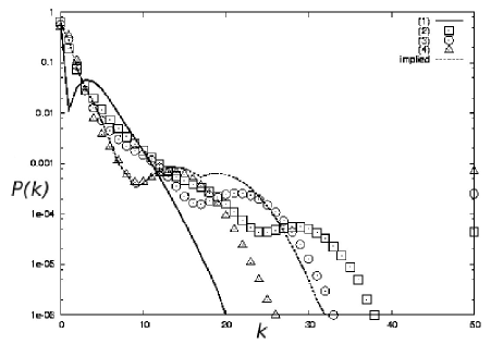
Figure 7: Plot of default probability distribution for the four cases and the implied distribution on August 30, 2005.

We calibrate our model based on the premiums of iTraxx-CJ (Series 2). iTraxx-CJ is an equally weighted portfolio of $N=50$ credit default swaps (CDSs) on Japanese companies. The interesting point is that they are divided into several parts (called as ”tranches”). The tranches have priorities that are defined by the attachment point $a_{L}$ and detachment point $a_{H}$. The protection seller agrees to cover all the losses between $a_{L}K_{Total}$ and $a_{H}K_{Total}$, where $K_{Total}$ is the initial total notional of the portfolio. That is, if the loss is below $a_{L}K_{Total}$, the tranche does not cover it. Only when it exceeds $a_{L}K_{Total}$, the tranche begins to cover it. If it exceeds $a_{H}K_{Total}$, the notional becomes zero. iTraxx-CJ has five tranches and their attachment and detachment points are $\{0\%,3\%\}$, $\{3\%,6\%\}$,$\{6\%,9\%\}$, $\{9\%,12\%\}$, and $\{12\%,22\%\}$. In addition, there is an index with $\{0\%,100\%\}$. We denote these tranches as $\{a_{L}^{i},a_{H}^{i}\}(\hskip 2.84544pti=1,2,\cdots,6)$ and the initial notional as $N_{0}^{i}=(a_{H}^{i}-a_{L}^{i})\times K_{Total}$.

The premium of these tranches depends on the expectation values of the final notional principal $<N_{T}^{i}>$, where $<\hskip 14.22636pt>$ denotes the average over the probability loss functions of the portfolio. If there are $k$ defaults, the loss is expressed as the difference of the notional principal time and $k$ times the recovery rate $R$, set at $35\%$, subtracted from 1. The final notional principal for the $i-$th tranche is

$$N_{T}^{i}(k)=\left\{\begin{array}[]{cc}N_{0}^{i}&k<\lceil\frac{a_{L}^{i}N}{1-R}\rceil\\ a_{H}N-k(1-R)&\lceil\frac{a_{L}^{i}N}{1-R}\rceil\leq k<\lceil\frac{a_{H}^{i}N}{1-R}\rceil\\ 0&k\geq\lceil\frac{a_{H}^{i}N}{1-R}\rceil.\\ \end{array}\right.$$ (33)

Here, $\lceil x\rceil$ denotes the smallest integer greater than $x$.

The premiums of the tranches $s_{i}$ and of the upfront $U_{i}$ are determined as follows;

$$U_{i}N_{0}^{i}+T<N_{T}^{i}>s_{i}e^{-rT}+(N_{0}^{i}-<N_{T}^{i}>)\frac{s_{i}T}{2}e^{-r\frac{T}{2}}$$ (34)

$$= (N_{0}^{i}-<N_{T}^{i}>)e^{-r\frac{T}{2}}.$$

Here, $r$ is the risk-free rate of interest and we set $r=1\%$. The left-hand side represents the expected payoff of the contact and the right-hand side represents the expected loss due to defaults.[15] Generally, $U_{i}=0$ for $i\geq 2$ and $s_{1}=3\%$.

The premiums include information about the credit market expectations regarding the probability loss functions. From these premiums, it is possible to infer the probability loss function, which is called the “implied default distribution.” It describes the probability of $k$ defaults of 50 Japanese companies. We denote it by $P_{imp}(k)$. There are several ways to infer the implied distribution; in Fig.7, we indicate $P_{imp}(k)$ with a dotted line based on the maximum entropy principle. The default probability $P_{d}$ is estimated as $P_{d}=1.65\%$, and the default correlation $\rho$ is $\rho=6.8\%$. It decreases rapidly for small $k$; for $9\leq k\leq 20$, it is almost constant at $\simeq 0.1\%$. Thereafter, $P_{imp}(k)$ rapidly decays to zero. Details of the inference process are provided elsewhere.[11] Many probabilistic models have been proposed to date, however they only yield poor fits to the implied distribution. Here, we calibrate the model parameters $p,q$, and $q^{\prime}$ and study whether or not our model effectively fits $P_{imp}(k)$.

In the calibration, we equate the default probability $P_{d}$ and default correlation $\rho$ of the model with those of the implied ones. There are three parameters $p,q$, and $q^{\prime}$ in the model, while there is only one degree of freedom. We study $P(k)$ for the following four cases.

1. Default infection only (left): $q^{\prime}=0.0,q=0.054857$, and $p=0.004512$.

2. Recovery infection only (right): $q=0.0,q^{\prime}=0.421050$, and $p=0.818175$.

3. Default infection with recovery (right): $q=0.001,q^{\prime}=0.563790$, and $p=0.847362$.

4. Default infection with recovery (right): $q=0.002,q^{\prime}=0.723940$, and $p=0.864563$.

The $P(k)$ values for the above four cases are shown in Fig.7. In the first case, the model exhibits only the default infection mechanism $(q^{\prime}=0)$, and which is indicated with a solid line. $P(k)$ exhibits a sharp valley structure at $k=1$ and then decreases rapidly to zero at $k\simeq 20$. This profile is clearly different from that of the implied one. On the other hand, the model with the right solution $q^{\prime}>q$ and $p\sim 1$, where the recovery effect dominates over the default infection, the bulk profiles are smooth. They are depicted by the symbols $\square(q=0.0),\bigcirc(q=0.001)$, and $\triangle(q=0.002)$. Their profiles are closer to the implied one than that of the infection only case. As $q$ increases, the tail becomes short and fat. At $q=0.001$ and $q=0.002$, they look similar to the implied one. We consider the infectious recovery to be important to describe the implied default distribution in the framework of infectious models.

The $P(k)$ values for the right solutions (cases 2, 3, and 4) have another peak at $k=50$. The peak means the probability that all the 50 companies default simultaneously. The discrepancy from $P_{imp}(k)$ is not very serious, because the inference of the default distribution from market quotes depends on the details of the optimization process. Instead of the entropy maximum principle, if we use another method, the implied distribution might have a peak at $k=50$.

The reason why the peak appears at this position in the infectious models is that we need to set a large value of $p$ for obtaining the right solution. The probability that all 50 companies are bad is $p^{50}$, and it is non zero; in the case, the recovery infection does not occur because there are no good companies and $P(50)$ remains. On the other hand, the probability of $k<50$ bad companies and $50-k$ good companies is $P_{int}(k)={}_{50}C_{k}\cdot p^{k}(1-p)^{50-k}$. In this case, $50-k$ good companies support $k$ bad companies, and the resulting default number is far less than $k$. Intuitively, probability $P_{int}(k)$ for $k$ bad companies is shifted to the left and it changes to probability $P(k^{\prime})$ for $k^{\prime}<k$ defaults. As $q$ increases, in order to fix $P_{d}$ and $\rho$, we need to increase $p$ and $q^{\prime}$. The peak at $k=50$ becomes higher, and the shift of $P(k)$ to the left increases. As a result, $P(k)$ moves to the left.

In case 1 where only default infection occurs, the distribution shifts to the right in general. In the case of $k=0$ where there are no bad companies, the probability $(1-p)^{50}$ is maintained. The default infection does not occur and $P(k)$ has a peak at $k=0$.

We have also compared the premiums obtained using our model with the real values. The first row of Table 1 lists the quotes for iTraxx-CJ (Series 2) on August 30, 2005. In the second row, we show the premiums derived using our model with the parameters of the above four cases. We find that case (3) realizes the best match with the real premiums. In the table, we also list the premiums based on the Gaussian copula loss function, which is a standard model in financial engineering. [15] As the model parameter, we use the same $P_{d}$ and $\rho$ values as the implied one’s.

Premiums	$U_{1}$	$s_{2}$	$s_{3}$	$s_{4}$	$s_{5}$	$s_{6}$ (Index)
iTraxx-CJ	0.131330	0.008917	0.002850	0.002000	0.001400	0.002208
IDM 1	0.056668	0.024918	0.007940	0.001971	0.000190	0.002203
IDM 2	0.107641	0.013250	0.005137	0.002432	0.000809	0.002202
IDM 3	0.133617	0.008996	0.003695	0.002025	0.000798	0.002203
IDM 4	0.096937	0.014655	0.006025	0.002792	0.000815	0.002203
Gaussian Model	0.207827	0.004207	0.000078	0.000000	0.000000	0.002203

Table 1: Premiums for iTraxx-CJ (Series 2) on August 30, 2005, and those derived using our model.

5 Concluding remarks and future problems

We have generalized the infectious default model by incorporating an infectious recovery effect. We have explicitly obtained the default probability function $P(k)$ for $k$ defaults as a function of model parameters $p,q$, and $q^{\prime}$. We have considered the continuous limit and obtained the probability density function $p(x)$ for the default ratio $x=\frac{k}{N}$. We have understood the oscillating behavior of $p(x)$ by decomposing it, as expressed by eq.(26). $p(x)$ is expressed as a superposition of the occurrence of $n$ bad obligors and the following default infection. The former follows a Poisson distribution and the latter obeys a normal distribution. The normal distributions have narrow peaks of width $\sim\frac{1}{\sqrt{N}}$, which appear in the oscillating behavior of $p(x)$. We have compared the obtained $P(k)$ with the implied one $P_{imp}(k)$ inferred from the iTraxx-CJ quotes.

By calibrating the model parameters, the profiles appear similar with regard to the bulk shape. However, $P(k)$ has a peak at $k=50$. We provide an intuitive explanation for it. We note that the principal features of our model are solvability, fitness for the implied distribution, and the model can be expressed as a superposition of the Poisson distributions with only three parameters.

In the future, we should study the time evolution of our model. One possibility is that we prepare an initial configuration of $S_{i}(t=0)$, whose time evolution is expressed as

$$S_{i}(t+1)=S_{i}(t)\Pi_{j\neq i}(1-Y_{ij}^{\prime}(t)(1-S_{j}(t)))+(1-S_{i}(t))(1-\Pi_{j\neq i}(1-Y_{ij}(t)S_{j}(t))).$$ (35)

$Y_{ij}(t)$ and $Y^{\prime}_{ij}(t)$ are independent Bernoulli-type variables at each time $t$, and the configuration of $S_{j}(t)$ is mapped to a new configuration $S_{i}(t+1)$. In the original problem, the binomial distribution $\mbox{Bi}(N,p)$ for $X_{i}$ is transformed into a singular oscillating $P(k)$. We can expect more dynamic and complex behaviors. Furthermore, in addition to the two-body interaction $Y_{ij},Y^{\prime}_{ij}$, three-body or many body interactions might be interesting; this can be achieved by maintaining the integrability of the model, to determine the extent, to which such a generalization is possible. In the continuous limit, the model with a continuous mixing function $f(p)$ should be searched.

The model is defined on the complete graph, where all nodes are interconnected. However, in recent times, the industry networks have been extensively studied and it has been shown that they have complex structures.[19, 20] The behavior of the model on such realistic networks is interesting. In addition, the relation between this model and the contact process[21, 22, 23] should be clarified. Despite the evident similarity of our model to the contact process, the infectious model proposes a new approach to the description of infection. It may be that we can obtain the attribute of the contact process from the infectious models by considering some limit.

References

- [1] R. S. Mantegna and H. E. Stanley: An Introduction to Econophysics (Cambridge University Press, 2000).
- [2] D. Challet, M. Marsili and Y. Zhang: Minority Games (Oxford University Press, 2005).
- [3] A. Aleksiejuk and J.A. Holyst: Physica A299 (2001) 198.
- [4] S. Jafarey and G.Iori: Physica A299 (2001) 205.
- [5] T. Lei and R. J. Hawkins: Phys. Rev. E65 (2002) 056119.
- [6] K. Kiyono, Z. R. Struik and Y. Yamamoto: Phys. Rev. Lett. 96 (2006) 068701.
- [7] T. Mizuno, H. Takayasu and M. Takayasu: arXiv:physics/0608115.
- [8] M. Davis and V. Lo: Quantitative Finance 1 (1999) 382.
- [9] K. Kitsukawa, S. Mori and M. Hisakado: Physica A368 (2006) 191.
- [10] M. Hisakado, K. Kitsukawa and S. Mori: J. Phys. A39(2006) 15365.
- [11] S. Mori, K. Kitsukawa and M. Hisakado: arXiv:physics/0609093.
- [12] S. Mori, K. Kitsukawa and M. Hisakado: arXiv:physics/0603036.
- [13] M. Bakkaloglu, J. J. Wylie, and C. Worg, G. R. Gonger: Technical Report CMU-CS-02-129, Carnegie Mellon University (2002).
- [14] P. J. Schönbucher: Credit Derivatives Pricing Models : Model, Pricing and Implementation (U.S. John Wiley & Sons) 2003.
- [15] J. Hull and A. White: Valuing Credit Derivatives Using an Implied Copula Approach, Working Paper (University of Toronto) 2006.
- [16] De Finetti: (Wiley, 1974).
- [17] J. F. C. Kingman: Ann. Probability 6 (1978) 183.
- [18] Y. S. Chow and H. Teicher: (Springer-Verlag, New York, 1978).
- [19] R. Albert and A. L. Barabasi: Rev. Mod. Phys. 74 (2002) 47.
- [20] W. Souma, Y. Fujiwara and H. Aoyama: Physica A324 (2003) 396.
- [21] N. Masuda, N. Konno and K. Aihara: Phys. Rev. E69 (2004) 031917.
- [22] R. Pastor-Satorras and A. Vespignani: Phys. Rev. Lett. 86 (2001) 3200.
- [23] R. B. Dchinszi: Math. Biosci. 173 (2001) 25.