Ultracold atom-molecule collisions and bound states in magnetic fields:
tuning zero-energy Feshbach resonances in He-NH (${}^{3}\Sigma^{-}$)

Abstract

We have generalized the BOUND and MOLSCAT packages to allow calculations in basis sets where the monomer Hamiltonians are off-diagonal and used the new capability to carry out bound-state and scattering calculations on ³He-NH and ⁴He-NH as a function of magnetic field. Following the bound-state energies to the point where they cross thresholds gives very precise predictions of the magnetic fields at which zero-energy Feshbach resonances occur. We have used this to locate and characterize two very narrow Feshbach resonances in ³He-NH. Such resonances can be used to tune elastic and inelastic collision cross sections, and sweeping the magnetic field across them will allow a form of quantum control in which separated atoms and molecules are associated to form complexes. For the first resonance, where only elastic scattering is possible, the scattering length shows a pole as a function of magnetic field and there is a very large peak in the elastic cross section. For the second resonance, however, inelastic scattering is also possible. In this case the pole in the scattering length is dramatically suppressed and the cross sections show relatively small peaks. The peak suppression is expected to be even larger in systems with stronger inelasticity. The results suggest that calculations on ultracold molecular inelastic collisions may be much less sensitive to details of the potential energy surface than has been believed.

I Introduction

Over the last 5 years, it has become possible to control the behavior of ultracold atomic gases by tuning the interactions between atoms using applied magnetic fields Hutson and Soldán (2006); Köhler et al. (2006). Notable successes have included the controlled implosion of Bose-Einstein condensates Roberts et al. (2001) and the production of molecules in both bosonic Donley et al. (2002); Herbig et al. (2003); Xu et al. (2003); Dürr et al. (2004) and fermionic Regal et al. (2003); Strecker et al. (2003); Cubizolles et al. (2003); Jochim et al. (2003a) quantum gases. Long-lived molecular Bose-Einstein condensates of fermion dimers have been produced Jochim et al. (2003b); Zwierlein et al. (2003); Greiner et al. (2003), and the first signatures of ultracold triatomic Kraemer et al. (2006) and tetraatomic Chin et al. (2005) molecules have been observed. The new capabilities in atomic physics have had important applications in other areas: for example, the tunability of atomic interactions has allowed exploration of the crossover between Bose-Einstein condensation (BEC) and Bardeen-Cooper-Schrieffer (BCS) behavior in dilute gases Bartenstein et al. (2004); Regal et al. (2004); Zwierlein et al. (2004).

In parallel with the work on atomic gases, there have been intense efforts to cool molecules directly from high temperature to the ultracold regime. Molecules such as NH₃, OH and NH have been cooled from room temperature to the milliKelvin regime by a variety of methods including buffer-gas cooling Weinstein et al. (1998); Egorov et al. (2004) and Stark deceleration Bethlem and Meijer (2003); Bethlem et al. (2006). Directly cooled molecules have been successfully trapped at temperatures around 10 mK, and there are a variety of proposals for ways to cool them further, including evaporative cooling, sympathetic cooling and cavity-assisted cooling Domokos and Ritsch (2002); Chan et al. (2003).

The possibility of controlling molecular interactions in the same way as atomic interactions is of great interest. Several groups have begun to explore the effects of external fields on ultracold molecular collisions Krems (2005). Volpi and Bohn Volpi and Bohn (2002) investigated collisions of ¹⁷O₂ with He and found a very strong enhancement of spin-flipping cross sections even for weak magnetic fields. Krems et al. Krems et al. (2003) and Cybulski et al. Cybulski et al. (2005) investigated spin-flipping collisions of NH with He and found a similar dependence on magnetic field. Krems and Dalgarno Krems and Dalgarno (2004a, b) elaborated the formal theory of scattering in a magnetic field for a variety of atom-molecule and molecule-molecule cases involving molecules in ${}^{2}\Sigma$ and ${}^{3}\Sigma$ states. Ticknor and Bohn Ticknor and Bohn (2005a) investigated OH+OH collisions and found that in this case magnetic fields could suppress inelastic collisions. Lara et al. Lara et al. (2006a, b) investigated the very complicated case of OH + Rb collisions, using basis sets designed to allow a magnetic field to be applied, though their initial calculations were for zero field.

The effects of electric fields have also been investigated. Avdeenkov and Bohn Avdeenkov and Bohn (2002, 2003) investigated OH-OH collisions in the presence of electric fields that caused alignment of the molecules. They identified novel field-linked states arising from long-range avoided crossings between effective potential curves in the presence of a field Avdeenkov and Bohn (2003); Avdeenkov et al. (2004); Avdeenkov and Bohn (2005); Ticknor and Bohn (2005b). Avdeenkov et al. Avdeenkov et al. (2006) have also investigated the effects of very high electric fields on collisions of closed-shell molecules. Very recently, Tscherbul and Krems Tscherbul and Krems (2006) have explored the effect of combined electric and magnetic fields on He-CaH collisions and observed significant suppression of spin-flipping transitions at high electric fields in the cold regime ($\sim 0.5$ K).

An important technique used to produce dimers in ultracold atomic gases is magnetic tuning across Feshbach resonances Hutson and Soldán (2006); Köhler et al. (2006). A Feshbach resonance Feshbach (1958, 1962) occurs whenever a bound state associated with one potential curve lies above the threshold for another curve. The resonance thus corresponds to a level embedded in a continuum, which is a quasibound state. In the atomic case, the thresholds that produce low-energy Feshbach resonances are associated with different hyperfine states of the interacting atoms. It is often possible to tune a resonance across threshold (from above or below) by applying a magnetic field. This produces an avoided crossing between atomic and molecular states. If the magnetic field is tuned across the resonance slowly enough to follow the avoided crossing adiabatically, pairs of atoms can be converted into molecules or vice versa.

Molecules have a much richer energy level structure than atoms, and there are many additional types of Feshbach resonance. In particular, rotational Feshbach resonances can occur Ashton et al. (1983); Hutson and Le Roy (1983) and have significant influences on ultracold molecular collisions Bohn et al. (2002). Other small energy level splittings, such as spin-rotation and $\Lambda$-doubling, can also cause resonances in molecular scattering. It is of great interest to characterize such resonances and their field-dependence, both to understand their influence on collision cross sections and to prepare the ground for experiments that associate molecules by Feshbach resonance tuning.

The NH molecule is particularly topical in cold and ultracold molecule studies. It is a dipolar molecule with a ${}^{3}\Sigma^{-}$ ground state, so it is both electrostatically and magnetically trappable. It has been cooled by beam-loaded buffer-gas cooling Egorov et al. (2004) and is a promising candidate for molecular beam deceleration and trapping van de Meerakker et al. (2003). Krems et al. Krems et al. (2003) and Cybulski et al. Cybulski et al. (2005) have calculated potential energy surfaces for He-NH and used them in scattering calculations. Cybulski et al. also calculated zero-field bound states of the He-NH Van der Waals complex. An electronic excitation spectrum of the Van der Waals complex has been observed by Kerenskaya et al. Kerenskaya et al. (2004). Soldán and Hutson Soldán and Hutson (2004) have investigated the interaction potentials for NH with Rb, and Dhont et al. Dhont et al. (2005) have developed interaction potential energy surfaces for NH-NH in the singlet, triplet and quintet states.

In the present article we describe the first calculations of the bound states of a Van der Waals complex in a magnetic field. We show how such calculations can be used to locate zero-energy Feshbach resonances as a function of applied field. Elastic and inelastic cross sections can then be tuned by sweeping the field across the Feshbach resonance. Such field sweeps could also be used to transfer unbound atom-molecule or molecule-molecule pairs into bound states of the corresponding complex.

A remarkable conclusion of the present paper is that, in the presence of inelastic scattering, the poles in scattering lengths that characterize low-energy Feshbach resonances in atomic systems Köhler et al. (2006) are dramatically suppressed and elastic and inelastic cross sections show relatively small peaks as resonances cross thresholds. The numerical results obtained here allow us to test analytical formulae for this effect recently given by Hutson Hutson (2006).

II Methods for bound-state calculations

We consider the case of an NH molecule interacting with a He atom in the presence of a magnetic field. The Hamiltonian for this in Jacobi coordinates $(R,\theta)$ is

$${\hat{H}}=-\frac{\hbar^{2}}{2\mu}R^{-1}\frac{d^{2}}{dR^{2}}R+\frac{\hat{L}^{2}}{2\mu R^{2}}+{\hat{H}}_{\rm mon}+{\hat{H}}_{\rm Z}+V(R,\theta),$$ (1)

where $\hat{L}^{2}$ is the space-fixed operator for end-over-end rotation, ${\hat{H}}_{\rm mon}$ is the Hamiltonian for the NH monomer, ${\hat{H}}_{\rm Z}$ is the Zeeman interaction and $V(R,\theta)$ is the intermolecular potential. For simplicity we consider the NH molecule to be a rigid rotor, but the generalization to include NH vibrations is straightforward. The NH monomer Hamiltonian is therefore

$${\hat{H}}_{\rm mon}=\hbar^{-2}b_{\rm NH}\hat{N}^{2}+{\hat{H}}_{\rm SN}+{\hat{H}}_{\rm SS},$$ (2)

where $b_{\rm NH}=16.343\;{\rm cm}^{-1}$ is the rotational constant of NH in its ground vibrational level Brazier et al. (1986),

$${\hat{H}}_{\rm SN}=\gamma\hat{N}\cdot\hat{S}$$ (3)

is the spin-rotation operator, and

$${\hat{H}}_{\rm SS}=\frac{2}{3}\lambda_{\rm SS}\left[\frac{4\pi}{5}\right]^{\frac{1}{2}}\sqrt{6}\sum_{q}(-1)^{q}Y_{2-q}(\hat{r})\left[S\otimes S\right]^{(2)}_{q}$$ (4)

is the spin-spin operator written in space-fixed coordinates Mizushima (1975). $\hat{N}$ and $\hat{S}$ are the operators for the rotational and spin angular momenta. The numerical values for the spin-rotation and spin-spin constants are $\gamma=-0.0055\;{\rm cm}^{-1}$ and $\lambda_{\rm SS}=0.920\;{\rm cm}^{-1}$ Mizushima (1975).

There are several basis sets that could be used to expand the eigenfunctions of Eq. (1). We consider two of them in the present work, which we refer to as the coupled and uncoupled basis sets. Both basis sets represent the end-over-end rotation with quantum numbers $|LM_{L}\rangle$, where $L$ is a rotational quantum number and $M_{L}$ is its projection onto the space-fixed $Z$ axis.

We use the convention that quantum numbers that describe a monomer are represented with lower-case letters, and reserve capital letters to describe states of the complex as a whole. In the absence of a magnetic field (or a perturbing atom), the rotational states of NH are approximately described by quantum numbers $n$, $s$ and $j$, where $n$ represents the mechanical rotational of NH, $s$ is the electron spin, and $j$ is the vector sum of $n$ and $s$. In the coupled representation for the He-NH problem, we use basis functions $|nsjm_{j}\rangle|LM_{L}\rangle$ that retain these monomer quantum numbers, with $m_{j}$ the projection of $j$ onto the space-fixed $Z$ axis. In the uncoupled representation, we use instead basis functions $|nm_{n}\rangle|sm_{s}\rangle|LM_{L}\rangle$, where $m_{n}$ and $m_{s}$ are the projections of $n$ and $s$ individually.

In both basis sets we use, the matrix elements of $\hat{L}^{2}$ are diagonal in all quantum numbers and are simply $\hbar^{2}L(L+1)$. The rotational part of the monomer Hamiltonian is also diagonal, with matrix elements $b_{\rm NH}n(n+1)$. The remaining matrix elements of the NH monomer Hamiltonian in the two basis sets are

$$\langle nsjm_{j}|{\hat{H}}_{\rm SN}|n^{\prime}sj^{\prime}m_{j}^{\prime}\rangle = \delta_{nn^{\prime}}\delta_{jj^{\prime}}\delta_{m_{j}m_{j}^{\prime}}\gamma(-1)^{n+j+s}\left[n(n+1)(2n+1)s(s+1)(2s+1)\right]^{\frac{1}{2}}\left\{\begin{array}[]{ccc}s&n&j\\ n&s&1\end{array}\right\};$$ (7)

$$\langle nsjm_{j}|{\hat{H}}_{\rm SS}|n^{\prime}sj^{\prime}m_{j}^{\prime}\rangle = \delta_{jj^{\prime}}\delta_{m_{j}m_{j}^{\prime}}\frac{2\sqrt{30}}{3}\lambda_{\rm SS}(-1)^{j+n^{\prime}+n+s}\left[(2n+1)(2n^{\prime}+1)\right]^{\frac{1}{2}}\left(\begin{array}[]{ccc}n&2&n^{\prime}\\ 0&0&0\end{array}\right)\left\{\begin{array}[]{ccc}s&n^{\prime}&j\\ n&s&2\end{array}\right\}$$ (12)

and

$$\langle sm_{s}|\langle nm_{n}|{\hat{H}}_{\rm SN}|n^{\prime}m_{n}^{\prime}\rangle|sm_{s}^{\prime}\rangle = \delta_{nn^{\prime}}\delta_{m_{n}m_{n}^{\prime}}\delta_{m_{s}m_{s}^{\prime}}\gamma m_{n}m_{s}$$ (13)

$$+ \left(\delta_{nn^{\prime}}\delta_{m_{n}m_{n}^{\prime}\pm 1}\delta_{m_{s}m_{s}^{\prime}\mp 1}\right)\frac{\gamma}{2}\left[n(n+1)-{m_{n}^{\prime}}(m_{n}^{\prime}\pm 1)\right]^{\frac{1}{2}}\left[s(s+1)-{m_{s}^{\prime}}(m_{s}^{\prime}\mp 1)\right]^{\frac{1}{2}};$$

$$\langle sm_{s}|\langle nm_{n}|{\hat{H}}_{\rm SS}|n^{\prime}m_{n}^{\prime}\rangle|sm_{s}^{\prime}\rangle = \frac{2\sqrt{30}}{3}\lambda_{\rm SS}(-1)^{s-m_{s}-m_{n}}\left[(2n+1)(2n^{\prime}+1)\right]^{\frac{1}{2}}\left[s(s+1)(2s+1)\right]\left(\begin{array}[]{ccc}n&2&n^{\prime}\\ 0&0&0\end{array}\right)$$ (23)

$$\times\left\{\begin{array}[]{ccc}1&1&2\\ s&s&s\end{array}\right\}\sum_{q}(-1)^{q}\left(\begin{array}[]{ccc}n&2&n^{\prime}\\ -m_{n}&-q&m_{n}^{\prime}\end{array}\right)\left(\begin{array}[]{ccc}s&2&s\\ -m_{s}&q&m_{s}^{\prime}\end{array}\right).$$

It may be noted that ${\hat{H}_{\rm mon}}$ is approximately diagonal in the coupled representation but not in the uncoupled representation. In the coupled representation, the only off-diagonal terms are matrix elements of ${\hat{H}_{\rm SS}}$ that couple different rotational states with $\Delta n=\pm 2$.

The Zeeman Hamiltonian for NH, neglecting rotational and anisotropic spin terms Brown and Carrington (2003) is

$${\hat{H}}_{\rm Z}=g_{\rm e}\mu_{\rm B}{\hat{B}}\cdot{\hat{S}},$$ (24)

where $g_{\rm e}$ is the $g$-factor for the electron, $\mu_{\rm B}$ the Bohr magneton and $\hat{B}$ is the magnetic field vector. The matrix elements of this operator are

$$\langle nsjm_{j}|{\hat{H}}_{\rm Z}|n^{\prime}sj^{\prime}m_{j}^{\prime}\rangle = \delta_{nn^{\prime}}\delta_{m_{j}m_{j}^{\prime}}g_{\rm e}\mu_{\rm B}B(-1)^{n+s-m_{j}+1}\left[s(s+1)(2s+1)(2j+1)(2j^{\prime}+1)\right]^{\frac{1}{2}}$$ (29)

$$\times\left(\begin{array}[]{ccc}j&1&j^{\prime}\\ -m_{j}&0&m_{j}\end{array}\right)\left\{\begin{array}[]{ccc}s&j^{\prime}&n\\ j&s&1\end{array}\right\}$$

and

$$\langle sm_{s}|\langle nm_{n}|{\hat{H}}_{\rm Z}|n^{\prime}m_{n}^{\prime}\rangle|sm_{s}^{\prime}\rangle=\delta_{nn^{\prime}}\delta_{m_{n}m_{n}^{\prime}}\delta_{m_{s}m_{s}^{\prime}}g_{\rm e}\mu_{\rm B}Bm_{s},$$ (30)

where the magnetic field direction has been chosen as the $Z$ axis and $B$ is the field strength. This is diagonal in the uncoupled representation but not in the coupled representation.

The intermolecular potential is conveniently expanded in Legendre polynomials,

$$V(R,\theta)=\sum_{\lambda}V_{\lambda}(R)P_{\lambda}(\cos\theta).$$ (31)

The matrix elements of the Legendre polynomials in the coupled and uncoupled basis sets are

$$\langle LM_{L}|\langle nsjm_{j}|P_{\lambda}(\cos\theta)|n^{\prime}sj^{\prime}m_{j}^{\prime}\rangle|L^{\prime}M_{L}^{\prime}\rangle = \left[(2n+1)(2n^{\prime}+1)(2j+1)(2j^{\prime}+1)(2L+1)(2L^{\prime}+1)\right]^{\frac{1}{2}}$$ (43)

$$\times\left(\begin{array}[]{ccc}n&\lambda&n^{\prime}\\ 0&0&0\end{array}\right)\left(\begin{array}[]{ccc}L&\lambda&L^{\prime}\\ 0&0&0\end{array}\right)\sum_{m_{\lambda}}(-1)^{s+j+j^{\prime}+\lambda+m_{\lambda}-M_{L}-m_{j}}$$

$$\times\left(\begin{array}[]{ccc}L&\lambda&L^{\prime}\\ -M_{L}&-m_{\lambda}&M_{L}^{\prime}\end{array}\right)\left(\begin{array}[]{ccc}j&\lambda&j^{\prime}\\ -m_{j}&m_{\lambda}&m_{j}^{\prime}\end{array}\right)\left\{\begin{array}[]{ccc}j&j^{\prime}&\lambda\\ n^{\prime}&n&s\end{array}\right\}$$

and

$$\langle LM_{L}|\langle sm_{s}|\langle nm_{n}|P_{\lambda}(\cos\theta)|n^{\prime}m_{n}^{\prime}\rangle|sm_{s}^{\prime}\rangle|L^{\prime}M_{L}^{\prime}\rangle = \delta_{m_{s}m_{s}^{\prime}}\left[(2n+1)(2n^{\prime}+1)(2L+1)(2L^{\prime}+1)\right]^{\frac{1}{2}}$$ (53)

$$\times\left(\begin{array}[]{ccc}n&\lambda&n^{\prime}\\ 0&0&0\end{array}\right)\left(\begin{array}[]{ccc}L&\lambda&L^{\prime}\\ 0&0&0\end{array}\right)\sum_{m_{\lambda}}(-1)^{m_{\lambda}-M_{L}-m_{n}}$$

$$\times\left(\begin{array}[]{ccc}L&\lambda&L^{\prime}\\ -M_{L}&-m_{\lambda}&M_{L}^{\prime}\end{array}\right)\left(\begin{array}[]{ccc}n&\lambda&n^{\prime}\\ -m_{n}&m_{\lambda}&m_{n}^{\prime}\end{array}\right).$$

This is off-diagonal in both representations.

We solve the bound-state Hamiltonian by a coupled channel method Hutson (1994). Denoting a complete set of channel quantum numbers $(n,s,j,m_{j},L,M_{L})$ or $(n,m_{n},s,m_{s},L,M_{L})$ by $i$, we expand the total wavefunction

$$\Psi=R^{-1}\sum_{i}\Phi_{i}(\hat{R},\hat{r})\chi_{i}(R),$$ (54)

where $(\hat{R},\hat{r})$ represents all coordinates except the intermolecular distance $R$ and the channel functions $\Phi_{i}(\hat{R},\hat{r})$ are the corresponding basis functions of the coupled or uncoupled basis sets. Substituting this expansion into the total Schrödinger equation yields a set of coupled differential equations for the radial functions $\chi_{i}(R)$,

$$\left[-\frac{\hbar^{2}}{2\mu}\frac{d^{2}}{dR^{2}}+\frac{\hbar^{2}L(L+1)}{2\mu R^{2}}-E\right]\chi_{i}(R)=-\sum_{i^{\prime}}\biggl{[}\langle i|{\hat{H}}_{\rm mon}+{\hat{H}}_{\rm Z}+V(R,\theta)|i^{\prime}\rangle\biggr{]}\chi_{i^{\prime}}(R).$$ (55)

In the present work we solve the coupled equations to find bound states using the BOUND program Hutson (1993), which uses the algorithms described in ref. Hutson, 1994. For $N$ channels there are $N$ coupled equations. However, it is actually necessary to propagate a set of $N$ linearly independent solutions, so $\chi(R)$ is an $N\times N$ matrix. The log-derivative matrix $Y=(d\chi/dR)\chi^{-1}$ is propagated outwards from $R_{\rm min}$ and inwards from $R_{\rm max}$ to a common matching point $R_{\rm mid}$ in the classically allowed region of the potential using Johnson’s algorithm Johnson (1973). This is done for a series of trial energies. If the energy is an eigenvalue of the Hamiltonian, the determinant of the log-derivative matching matrix $Y_{\rm match}=Y_{\rm in}-Y_{\rm out}$ is zero. Bound states are located by searching for zeroes of eigenvalues of $Y_{\rm match}$ as a function of energy. The log-derivative method provides a generalised node count Johnson (1978); Hutson (1994) which increases by one at each energy eigenvalue, and this allows us to use bisection to identify regions of energy that contain a bound state. The actual convergence on an energy eigenvalue uses the secant method, which gives quadratic convergence.

Version 5 of the BOUND program Hutson (1993) contained an interface to allow new basis sets to be added, but could only handle basis sets in which the monomer Hamiltonian was diagonal. We have extended the program to remove this restriction and implemented the coupled and uncoupled basis sets described above. We have also built in new loops over external fields to simplify calculations on Stark and Zeeman effects.

III Results of bound-state calculations

We have carried out bound-state calculations on ⁴He-NH and ³He-NH using the potential energy surface of Krems et al. Krems et al. (2003) (described in more detail as potential 2 of Cybulski et al. Cybulski et al. (2005)). The basis set included all functions with $n\leq 8$ and $L\leq 7$. The coupled equations were propagated outwards from 1.8 Å to 3.57 Å and inwards from 16.0 Å to 3.57 Å using a log-derivative sector size of 0.025 Å. WKB boundary conditions were applied in each channel at $R_{\rm max}$ to improve the convergence.

In zero field, the levels of He-NH are characterized by the total angular momentum $\cal J$, which is the vector sum of $j$ and $L$. The total parity is also conserved and is given by $(-1)^{n+L+1}$. Since the lowest levels of NH have $n=0$, $j=s=1$ and ${\cal J}=L$, $L\pm 1$. The three different ${\cal J}$ levels corresponding to each value of $L$ are very close together: the separation is only about 10^-3 cm^-1 for $L=1$. The angular momentum coupling scheme corresponds to case (B) of Dubernet, Flower and Hutson Dubernet et al. (1991).

The field-free energies of He-NH on this potential have been calculated previously by Cybulski et al. Cybulski et al. (2005). Our results agree with theirs to $\pm 10^{-4}$ cm^-1 for the levels with $L=0$ to 2, but are approximately 0.0014 cm^-1 lower for the $L=3$ levels of ⁴He-NH, which are bound by only 0.765 cm^-1. We attribute the difference to lack of convergence of the radial basis set used in their calculations. The results obtained from our program with the coupled and uncoupled basis sets are identical to $\pm 10^{-9}$ cm^-1, which confirms the correctness of the code.

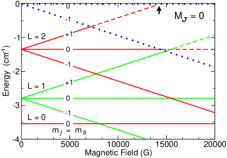
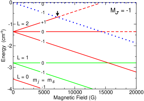
Figure 1: Bound-state energy levels for ³He-NH for $M_{\cal J}=0$ (upper panel) and $M_{\cal J}=-1$ (lower panel) as a function of magnetic field $B$. Levels of odd parity are shown in red and levels of even parity in green. Dissociation thresholds are shown as dotted blue lines and quasibound levels are shown as dashed lines. The arrows show the positions at which levels cross $L=0$ thresholds.

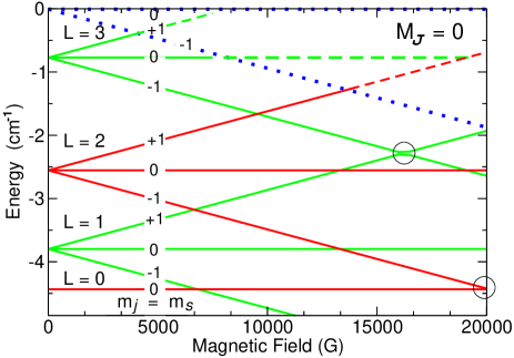
Figure 2: Bound-state energy levels for ⁴He-NH for $M_{\cal J}=0$ as a function of magnetic field $B$. Levels of odd parity are shown in red and levels of even parity in green. Dissociation thresholds are shown as dotted blue lines and quasibound levels are shown as dashed lines. Avoided crossings are circled.

In the presence of a field, $\cal J$ is very quickly destroyed. The only rigorously good quantum numbers in a magnetic field are parity and $M_{\cal J}=m_{j}+M_{L}=m_{n}+m_{s}+M_{L}$. The bound-state energies for levels correlating with $n=0$ for ³He-NH with $M_{\cal J}=0$ and $-1$ are shown in Fig. 1. Each level splits into components that can be labelled with the approximate quantum numbers $m_{n}=0$ and $m_{s}=0$, $\pm 1$. $L$ remains an essentially good quantum number except in the vicinity of the avoided crossings. The major difference between $M_{\cal J}$ values is that some $m_{s}$ levels are missing for $M_{\cal J}\neq 0$, but there are also small shifts of all the energy levels. A similar plot for ⁴He-NH with $M_{\cal J}=0$ is shown in Fig. 2.

As expected, the Zeeman effect is generally quite linear for He-NH in the range of fields studied. This is because for $n=0$ the only off-diagonal terms are those of $V(R,\theta)$ and $\hat{H}_{\rm SS}$ that mix in excited $n$ levels, and the spacing between the $n=0$ and $n=1$ levels for NH is around 32.6 cm^-1. Nevertheless, there are avoided crossings where levels of the same $M_{\cal J}$ and parity but different $m_{s}$ cross. Expanded views of the energy level diagrams in the region of avoided crossings are shown for ⁴He in Fig. 3 and for ³He in Fig. 4. It may be seen that in this system the crossings are very tightly avoided, with spacings at the crossing points of $\Delta E=5.2\times 10^{-4}$ cm^-1 and $\Delta E=2.0\times 10^{-3}$ cm^-1 for ⁴He and $\Delta E=1.5\times 10^{-3}$ cm^-1 for ³He.

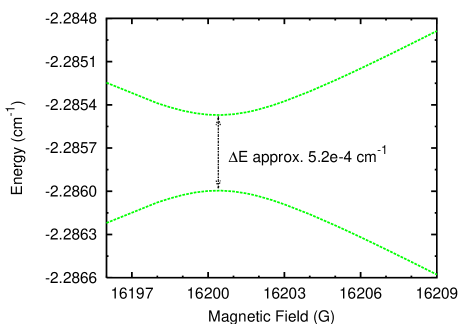
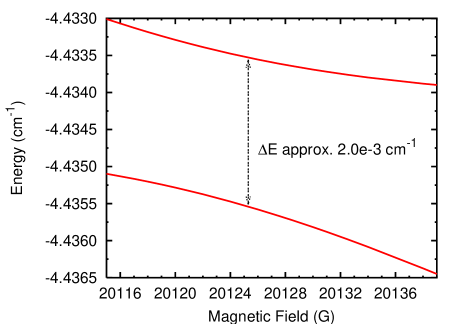
Figure 3: Avoided crossing between levels with $m_{s}=+1$ and $m_{s}=-1$ (upper panel) and between levels with $m_{s}=0$ and $m_{s}=-1$ (lower panel) for ⁴He-NH as a function of magnetic field $B$.

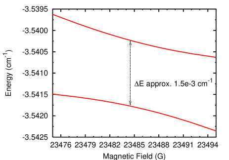
Figure 4: Avoided crossing between levels with $m_{s}=0$ and $m_{s}=-1$ for ³He-NH as a function of magnetic field $B$.

The reason that the crossings are so tightly avoided in this case is that there are no direct off-diagonal matrix elements between $n=0$ basis functions with different values of $m_{s}$. The dominant coupling is a second-order one of the form

$$\frac{\langle 001m_{s}|\hat{H}_{\rm SS}|2m_{n}1m_{s}^{\prime}\rangle\langle 2m_{n}1m_{s}^{\prime}|V_{2}|001m_{s}^{\prime}\rangle}{E_{n=2}-E_{n=0}},$$ (56)

where basis functions are represented $|nm_{n}sm_{s}\rangle$ and $m_{n}=m_{s}-m_{s}^{\prime}$. Such crossings will thus be more strongly avoided in systems with stronger anisotropy or smaller monomer rotational constant.

If matrix elements of $\hat{H}_{\rm SS}$ off-diagonal in $n$ are omitted, the avoided crossings still exist but are about a factor of 5 tighter. Under these circumstances they are caused by a third-order mechanism in which potential couplings mix in basis functions with $n>0$ (but the same values of $m_{s}$ and $m_{s}^{\prime}$) and these are connected by $\hat{H}_{\rm SS}$.

It should be noted that for levels with $n>0$ there are direct matrix elements of $\hat{H}_{\rm SS}$ and $\hat{H}_{\rm NS}$ that connect levels with different $m_{s}$ but the same $m_{j}$. This will produce more strongly avoided crossings where the separation is simply proportional to $\lambda_{\rm SS}$ (or $\gamma$ for ${}^{2}\Sigma$ monomers). This will be particularly important for ¹⁶O₂, which has an $n=1$ ground state.

The boundary conditions applied by the BOUND program are only correct for true bound states, below the lowest dissociation threshold. Above a threshold, the boundary conditions produce artificially quantized states. These are of two types: states that are predominantly in an open channel, which have no physical significance; and states that are predominantly in a closed channel, which correspond closely to quasibound states of the real system but with only an approximate open-channel (dissociative) component. The two types are very easy to tell apart: the open-channel states are closely parallel to a lower threshold, and inspection of the wavefunction confirms their parentage. The open-channel states have been omitted from Figs. 1 and 2. The closed-channel states are shown as dashed lines above the lowest threshold. They allow us to estimate very precisely where a bound or quasibound state crosses a threshold, and thus where a zero-energy resonance is expected in the scattering. This information will be used in section V below.

IV Methods for scattering calculations

The coupled equations needed for scattering calculations are identical to those for bound states. The only differences are that the energy $E$ is above one or more thresholds $E_{i}$ and that scattering boundary conditions are applied at long range. In the present work we solve the coupled equations for scattering using the MOLSCAT package Hutson and Green (1994). We have generalised MOLSCAT in the same way as BOUND to handle basis sets in which the monomer Hamiltonian is nondiagonal.

IV.1 Boundary conditions

The usual procedure for obtaining the scattering matrix $S$ from the log-derivative matrix $Y$ has been described by Johnson Johnson (1973). Each channel is either open, $E\geq E_{i}$ or closed, $E<E_{i}$. If matching takes place at a finite distance $R_{\rm max}$ where the wavefunction in the closed channels $(E<E_{i})$ has not decayed to zero, it is necessary to take account of the closed channels. The asymptotic form of the wavefunction is

$$\chi(R)=J(R)+N(R)K,$$ (57)

where $J(R)$ and $N(R)$ are diagonal matrices made up Riccati-Bessel functions for open channels and modified spherical Bessel functions for closed channels. If there are $N$ channels and $N_{\rm open}$ open channels, the $N\times N$ log-derivative matrix is converted into an $N\times N$ real symmetric $K$ matrix. The $S$ matrix is then obtained from the open-open submatrix, $K_{\rm oo}$, using the relationship

$$S=(I+{\rm i}K_{\rm oo})^{-1}(I-{\rm i}K_{\rm oo}),$$ (58)

where $I$ is an $N_{\rm open}\times N_{\rm open}$ unit matrix. However, the boundary conditions (57) are appropriate only in a basis set in which both $\hat{L}^{2}$ and the asymptotic Hamiltonian are diagonal. In our generalised version of MOLSCAT, the log-derivative matrix $Y$ is propagated in the primitive basis set (which is nondiagonal) and then transformed at $R_{\rm max}$ into a basis set that diagonalises $\hat{H}_{\rm mon}+\hat{H}_{\rm Z}$.

For the simple case of He-NH, the eigenvalues of $\hat{H}_{\rm mon}+\hat{H}_{\rm Z}$ are nondegenerate except at non-zero field. The transformation that diagonalises $\hat{H}_{\rm mon}+\hat{H}_{\rm Z}$ is thus unique. However, in more complicated cases with two structured collision partners it will be necessary to transform to a basis set that diagonalises $\hat{H}_{\rm mon,1}+\hat{H}_{\rm Z,1}$ and $\hat{H}_{\rm mon,2}+\hat{H}_{\rm Z,2}$ separately. Additional degeneracies arise at zero field, and resolving them may require diagonalisation of another operator such as $\hat{j}_{Z}$.

IV.2 Cross sections

The cross section for a transition $i\rightarrow f$ from initial state $i$ to final state $f$ is obtained from the square of the corresponding $T$ matrix element,

$$\sigma_{if}=\frac{\pi}{k^{2}}|T_{if}|^{2},$$ (59)

where $k$ is the incoming wave vector, $k^{2}=2\mu(E-E_{i})/\hbar^{2}$, and $T_{if}=\delta_{if}-S_{if}$. In general it is necessary to sum over all channels corresponding to the monomer levels of interest and over $S$ matrices obtained for different values of $M_{\cal J}$ and parity.

IV.3 Scattering lengths

In the ultracold regime, scattering properties are often described in terms of a complex scattering length $a=\alpha-{\rm i}\beta$ Balakrishnan et al. (1997); Bohn and Julienne (1997). The diagonal S-matrix element in the incoming channel $0$ may be written in terms of a complex phase shift $\delta$ Mott and Massey (1965),

$$S_{00}=\exp(2{\rm i}\delta)$$ (60)

and the complex scattering length is defined by

$$a=\frac{-\tan\delta}{k}.$$ (61)

Equivalently,

$$S_{00}=\frac{1-{\rm i}ka}{1+{\rm i}ka}.$$ (62)

The scattering length becomes constant at limitingly low energy. The elastic and total inelastic cross sections are Cvitaš et al. (2006)

$$\sigma_{\rm el}=\frac{4\pi|a|^{2}}{1+k^{2}|a|^{2}+2k\beta}$$ (63)

and

$$\sigma_{\rm inel}=\frac{4\pi\beta}{k(1+k^{2}|a|^{2}+2k\beta)}.$$ (64)

The scattering length is often given as

$$a=\lim_{k\rightarrow 0}\frac{1}{2{\rm i}}\frac{T_{00}}{k}.$$ (65)

However, this relies on a Taylor series expansion of $\exp(2{\rm i}\delta)$ that is valid only when $\delta\ll 1$. Across an elastic scattering resonance, $\delta$ changes by $\pi$ even at limitingly low energy, so Eq. 65 is inappropriate. In the present work we obtain scattering lengths numerically either by converting the low-energy S-matrix elements to complex phases using Eq. 60 and then the definition (61) or by using the equivalent identity

$$a=\frac{1}{{\rm i}k}\left(\frac{1-S_{00}}{1+S_{00}}\right).$$ (66)

IV.4 Resonant behavior

If there is only one open channel, then the phase shift $\delta$ is real and its behavior is sufficient to characterize a resonance. It follows a Breit-Wigner form as a function of energy,

$$\delta(E)=\delta_{\rm bg}+\tan^{-1}\left[\frac{\Gamma_{E}}{2(E_{\rm res}-E)}\right],$$ (67)

where $\delta_{\rm bg}$ is a slowly varying background term, $E_{\rm res}$ is the resonance position and $\Gamma_{E}$ is its width (in energy space). This corresponds to the $S$ matrix element describing a circle of radius 1 in the complex plane. In general the parameters $\delta_{\rm bg}$, $E_{\rm res}$ and $\Gamma_{E}$ are slow functions of energy, but this is neglected in the present work apart from threshold behaviour.

The resonance position $E_{\rm res}$ and the threshold energy $E_{\rm thresh}$ are both functions of magnetic field,

$$\frac{dE_{\rm res}}{dB}=\mu_{\rm res}\quad\hbox{and}\quad\frac{dE_{\rm thresh}}{dB}=\mu_{\rm thresh}.$$ (68)

We define $B_{\rm res}(E)$ as the field at which $E_{\rm res}=E$. For low kinetic energies, the width $\Gamma_{E}$ also depends on the field through its threshold dependence Timmermans et al. (1999),

$$\Gamma_{E}(E_{\rm kin})=2k\gamma_{E},$$ (69)

with constant reduced width $\gamma_{E}$. As a function of magnetic field at constant kinetic energy, the phase shift thus follows a form similar to Eq. 67,

$$\delta(B)=\delta_{\rm bg}+\tan^{-1}\left[\frac{\Gamma_{B}(E_{\rm kin})}{2(B_{\rm res}(E)-B)}\right].$$ (70)

The width $\Gamma_{B}(E_{\rm kin})$ is a signed quantity that is negative if the bound state tunes upwards through the energy of interest and positive if it tunes downwards,

$$\Gamma_{B}(E_{\rm kin})=\frac{\Gamma_{E}(E_{\rm kin})}{\mu_{\rm thresh}-\mu_{\rm res}}.$$ (71)

The background phase shift $\delta_{\rm bg}$ goes to zero as $k\rightarrow 0$ according to Eq. 61 (with constant finite $a_{\rm bg}$), but the resonant term still exists. The scattering length passes through a pole when $\delta=\left(n+\frac{1}{2}\right)\pi$. The scattering length follows the formula commonly used in atomic scattering Moerdijk et al. (1995),

$$a(B)=a_{\rm bg}\left[1-\frac{\Delta_{B}}{B-B_{\rm res}(E)}\right],$$ (72)

where $\Delta_{B}=-\Gamma_{B}/2ka_{\rm bg}=-\gamma_{B}/a_{\rm bg}$ and is independent of $k$ near threshold.

When there are several open channels, $\delta$ is in general complex. The quantity that then follows the Breit-Wigner form (67) or (70) is the S-matrix eigenphase sum Ashton et al. (1983), which is the sum of phases of the eigenvalues of the $S$ matrix. The eigenphase sum is real, because the $S$ matrix is unitary, so that all its eigenvalues have modulus 1. In practice the eigenphase sum is most conveniently calculated by diagonalising the real symmetric matrix $K_{\rm oo}$ and summing the inverse tangents of its eigenvalues.

If there is more than one open channel, the individual $S$ matrix elements still describe circles in the complex plane,

$$S_{ii^{\prime}}=S_{{\rm bg,}ii^{\prime}}-\frac{{\rm i}g_{Ei}g_{Ei^{\prime}}}{E-E_{\rm res}+{\rm i}\Gamma_{E}/2},$$ (73)

where $g_{Ei}$ is complex. The partial width for channel $i$ is $\Gamma_{Ei}=|g_{Ei}|^{2}$ and the radius of the circle in $S_{ii^{\prime}}$ is $|g_{Ei}g_{Ei^{\prime}}|/\Gamma_{E}$. The analogous expression as a function of magnetic field at constant kinetic energy is

$$S_{ii^{\prime}}=S_{{\rm bg,}ii^{\prime}}-\frac{{\rm i}g_{Bi}g_{Bi^{\prime}}}{B-B_{\rm res}+{\rm i}\Gamma_{B}/2},$$ (74)

where the energy-dependence of $B_{\rm res}$ and $\Gamma_{B}$ has been omitted to simplify notation. If $\Gamma_{E0}<\Gamma_{E}$ (or equivalently $|\Gamma_{B0}|<|\Gamma_{B}|$), the scattering length does not pass through a pole. In the low-energy threshold regime, $\Gamma_{B0}$ is proportional to $k$ and we may define an energy-independent reduced width $\gamma_{B0}$,

$$\Gamma_{B0}=2\gamma_{B0}k.$$ (75)

However, $\Gamma_{B}$ has inelastic contributions $\Gamma_{B}^{\rm inel}$ that are essentially energy-independent. Hutson Hutson (2006) has defined a resonant scattering length,

$$a_{\rm res}=\frac{2\gamma_{B0}}{\Gamma_{B}^{\rm inel}},$$ (76)

that characterizes the strength of the resonant contribution to the scattering at low energy. If $ka_{\rm res}\ll 1$, $S_{00}$ describes a circle of radius $2ka_{\rm res}$ in the complex plane as a resonance is tuned through threshold and the real part of the scattering length oscillates by $\pm a_{\rm res}/2$.

As will be seen below, for He + NH the inelastic scattering strongly suppresses the pole in the scattering length and the resonant oscillation in the scattering length is of quite small amplitude. The corresponding oscillations in the elastic and inelastic cross sections are also relatively weak.

V Results of scattering calculations

We have carried out scattering calculations on ⁴He-NH and ³He-NH using the potential energy surface of Krems et al. Krems et al. (2003). These calculations used a reduced basis set of functions with $n\leq 4$ and $L\leq 5$ to allow comparison with previous studies. The coupled equations were propagated outwards from 1.7 Å to 120.0 Å using Johnson’s log-derivative algorithm Johnson (1973) with a sector size of 0.025 Å.

We have verified that the new code gives identical scattering results for He-NH with the coupled and uncoupled basis sets. This confirms the correctness of the coding for the basis sets and the extraction of $S$ matrices. Our program also gives identical results to refs. Krems et al., 2003 and Cybulski et al., 2005 for scattering in a magnetic field.

It is of great interest to investigate the effect of zero-energy Feshbach resonances on low-energy molecular scattering as a function of magnetic field. However, a major problem is that the resonances can be very narrow, and locating the fields at which they occur is difficult and time-consuming. For example, in the He-NH problem we expect the coupling between bound and continuum states with different $m_{j}$ to be comparable to or smaller than that between bound states of different $m_{j}$. To a first approximation, the latter is the energy separation of the bound-state avoided crossings, which is around $10^{-3}$ cm^-1. Since the energy of a state with $m_{s}=\pm 1$ tunes by about $10^{-4}$ cm^-1/G, we expect the Feshbach resonances to be less (perhaps much less) than 10 G wide.

Fortunately, the bound-state capability described above provides a solution to this problem: we can extrapolate the bound-state energies to calculate the field at which they cross a threshold and then scan across a small range of fields in the vicinity. As an example, we searched for Feshbach resonances in ³He-NH. It may be seen in Fig. 1 that there is a ³He-NH bound state with $m_{s}=+1$ that crosses the $m_{s}=-1$ threshold at about 7200 G and the $m_{s}=0$ threshold at about 14300 G. Careful extrapolation of the bound-state energies with the basis set used for the scattering calculations gives more precise field estimates of 7168.750 G (for $M_{\cal J}=-1$) and 14340.36 G (for $M_{\cal J}=0$) respectively.

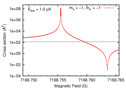
Figure 5: Elastic ($m_{s}=-1\rightarrow-1$) cross section for ³He-NH collisions in the vicinity of an elastic Feshbach resonance at a kinetic energy of $10^{-6}$ K.

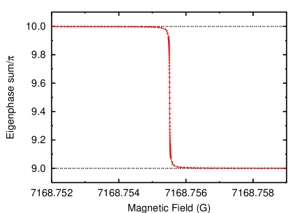
Figure 6: Phase shift for elastic ³He-NH collisions in the vicinity of an elastic Feshbach resonance at a kinetic energy of $10^{-6}$ K.

Care must be taken to use bound-state calculations for the correct values of $M_{\cal J}$ and parity. In the present case, we want s-wave resonances, with $L=0$ in the incoming channel. This requires $M_{\cal J}=m_{j}$ and even parity. Bound-state calculations with different values of $M_{\cal J}$ produce energies that cross threshold at different values of the field. In He-NH, which is a very weakly coupled system with almost linear Zeeman effects, the fields are only slightly different; for example, the crossing with the $m_{s}=0$ threshold occurs at 14345.40 G for $M_{\cal J}=-1$. Nevertheless, the difference can easily be enough to miss the resonance, and in more strongly coupled systems will be crucial.

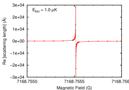
Figure 7: Scattering length for elastic ³He-NH collisions in the vicinity of an elastic Feshbach resonance, from calculations at a kinetic energy of $10^{-6}$ K.

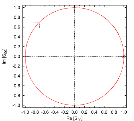
Figure 8: The circle of radius 1 in the complex plane described by the $L=0$ diagonal $S$ matrix element for elastic scattering in the vicinity of an elastic Feshbach resonance at a kinetic energy of $10^{-6}$ K. The cross shows the value far from resonance.

For ³He colliding with NH ($m_{s}=-1$) near 7169 G, only elastic scattering can occur. For $M_{\cal J}=-1$ and even parity, the present basis set gives 3 open channels with $L=0$, 2 and 4. Scattering into the $L>0$ channels is strongly suppressed by the centrifugal barriers. The elastic cross section is shown as a function of field in Fig. 5 and the corresponding eigenphase sum and scattering length are shown in Figs. 6 and 7. The peak in the cross section for kinetic energy $E_{\rm kin}=10^{-6}$ K is close to the value of $4\pi/k^{2}=1.2\times 10^{8}$ Å² characteristic of a pole in the scattering length. The peak shows an asymmetric Fano lineshape Fano (1961), with interference between a background term and a resonant term that interfere constructively on the low-field side of the resonance and destructively on the high-field side. The diagonal $S$ matrix element for $L=0$ describes a circle of radius 1 in the complex plane as the field is ramped across the resonance, as shown in Fig. 8. Fitting the eigenphase sum to Eq. 70 gives $\delta_{\rm bg}<0.001$, $B_{\rm res}=7168.7555$ G and $\Gamma_{B}=-1.65\times 10^{-5}$ G, while fitting the scattering length to Eq. 72 gives $a_{\rm bg}=3.19$ Å, $B_{\rm res}=7168.7555$ G and $\Delta_{B}=8.04\times 10^{-3}$ G. The widths $\Gamma_{B}$ and $\Delta_{B}$ are related by $\Gamma_{B}/2=-ka_{\rm bg}\Delta_{B}$. It may be seen that the bound-state calculation does indeed give a very precise estimate of the position of the zero-energy resonance.

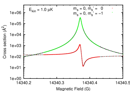
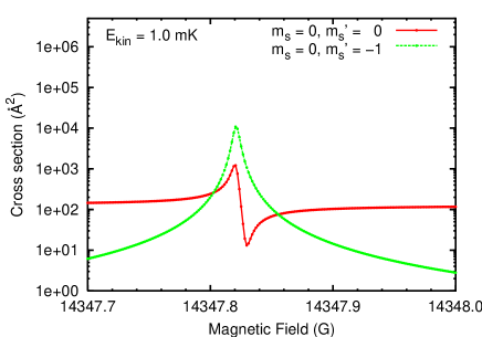
Figure 9: Elastic ($m_{s}=0\rightarrow 0$) and inelastic ($m_{s}=0\rightarrow-1)$ cross sections for ³He-NH collisions in the vicinity of an inelastic Feshbach resonance at kinetic energies of $10^{-6}$ K (upper panel) and $10^{-3}$ K (lower panel). The lines show the results of Eqs. LABEL:eqsigel and 79.

For ³He colliding with NH ($m_{s}=0$) near 14300 G, both elastic and inelastic scattering are possible. For $M_{\cal J}=0$ and even parity, our basis set gives 3 elastic channels ($m_{s}=0$ with $L=0$, 2 and 4) and 2 inelastic channels ($m_{s}=-1$ with $L=2$ and 4). However, the elastic channels with $L>0$ make no significant contributions at ultralow energies. Fig. 9 shows scans of the elastic ($m_{s}=0\rightarrow 0$) and total inelastic ($m_{s}=0\rightarrow-1)$ cross sections for kinetic energies of $10^{-6}$ K and $10^{-3}$ K. Once again the bound-state calculation gives a very precise estimate of the position of the zero-energy resonance. At $10^{-3}$ K the resonance is shifted slightly because a different field is needed to bring the bound state into resonance with the larger total energy. Apart from the shift, however, the cross sections behave as expected from the Wigner threshold laws: the elastic cross section is almost unchanged and the inelastic cross section scales with $k^{-1}$.

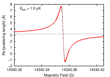
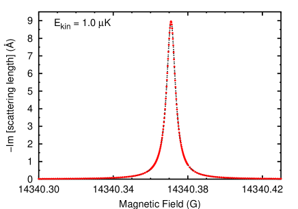
Figure 10: Real and imaginary parts of the scattering length for ³He-NH collisions in the vicinity of an inelastic Feshbach resonance, from calculations at a kinetic energy of $10^{-6}$ K. Upper panel: real part; lower panel: imaginary part. The lines show the results of Eq. 77.

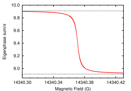
Figure 11: Eigenphase sum for inelastic ³He-NH collisions in the vicinity of an inelastic Feshbach resonance at a kinetic energy of $10^{-6}$ K.

A notable feature of Fig. 9 is that the elastic cross section does not peak at the very high value of $4\pi/k^{2}$ characteristic of a pole in the scattering length. The real and imaginary parts of the scattering length are shown in Fig. 10. Instead of rising to $\infty$, the scattering length oscillates with a peak at less than $+8$ Å. The eigenphase sum shows a sharp drop through $\pi$ as shown in Fig. 11, and fitting to Eq. 70 gives $B_{\rm res}=14340.371$ G and $\Gamma_{B}=-5.72\times 10^{-3}$ G. However, the phase change is distributed between several diagonal matrix elements.

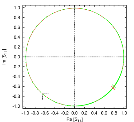
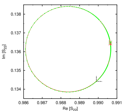
Figure 12: The circles described by diagonal $S$ matrix elements in the presence of inelastic scattering at $E_{\rm kin}=10^{-6}$ K (green) and $4\times 10^{-6}$ K (red). Upper panel: incoming wave (channel 0: $m_{s}=0$, $L=0$); center panel: (channel 1: $m_{s}=-1$, $L=2$); lower panel: (channel 2: $m_{s}=-1$, $L=4$). The crosses show values far from resonance.

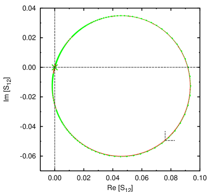
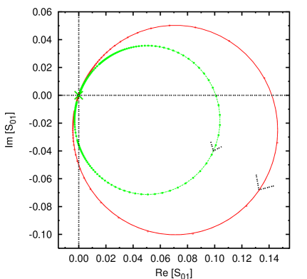
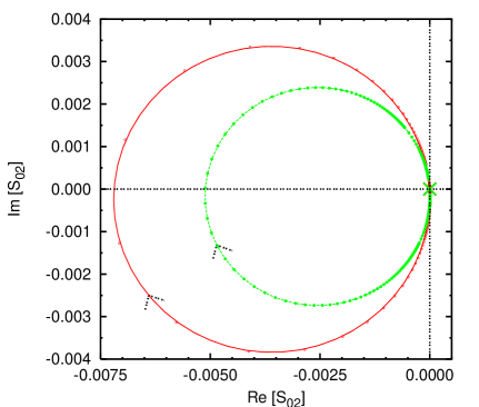
Figure 13: The circles described by the off-diagonal $S$ matrix elements for 3-channel scattering at $E_{\rm kin}=10^{-6}$ K (green) and $4\times 10^{-6}$ K (red). Channels are labeled as in Fig. 12. The crosses show values far from resonance.

The $S$ matrix elements are shown explicitly for two different energies, $E_{\rm kin}=10^{-6}$ K and $4\times 10^{-6}$ K, in Figs. 12 and 13. The corresponding values of $k$ differ by a factor of 2. It may be seen in Fig. 12 that the elastic $S$ matrix element for the low-energy incoming channel describes a small circle with a radius that depends linearly on $k$. For $E_{\rm kin}=10^{-6}$ K, the radius is only about 0.003. The other diagonal elements describe much larger circles that are almost independent of $k$, with background (nonresonant) $S$ matrix elements (shown by crosses) that are far from 1: these channels have substantial kinetic energy so are not governed by the Wigner threshold laws. The inelastic $S$ matrix elements are shown in Fig. 13, and it may be seen that those for incoming channel 0 describe circles with radius proportional to $k^{1/2}$.

Since $S_{00}$ describes a small circle in the complex plane, the corresponding complex phase $\delta$ given by Eq. 60 shows a relatively small oscillation that does not pass through $\pm\pi/2$. There is thus an oscillation but no pole in the scattering length $a$ (and no discontinuity in its sign). This explains why the peak in the elastic scattering cross section is much lower than the value of $4\pi/k^{2}$ expected when there is a pole in $a$.

The behavior observed here may be quantified in terms of the theory of Hutson Hutson (2006). Fitting the individual $S$ matrix elements at $E_{\rm kin}=10^{-6}$ K to Eq. 74 gives a partial width $\Gamma_{B0}=-1.646\times 10^{-5}$ G for the incoming channel and $\Gamma_{B1}=-5.693\times 10^{-3}$ G and $\Gamma_{B2}=-1.308\times 10^{-5}$ G for the two inelastic channels. We have verified numerically that $\Gamma_{B0}$ is proportional to $k$ and $\Gamma_{B1}$ and $\Gamma_{B2}$ are independent of it. With $k=3.219\times 10^{-4}$ Å^-1, this gives $\gamma_{B0}=0.02557$ G Å and $a_{\rm res}=8.96$ Å. The peaks in the scattering lengths in Fig. 10 are at $\alpha_{\rm max}=7.67$ Å, $\alpha_{\rm min}=-1.28$ Å, and $\beta_{\rm max}=8.96$ Å, which correspond to the theoretical predictions Hutson (2006), $\alpha^{\rm max}_{\rm min}=a_{\rm bg}\pm a_{\rm res}/2$ and $\beta_{\rm max}=a_{\rm res}$ with $a_{\rm bg}=3.19$ Å.

The shapes of the peaks in scattering lengths and cross sections also correspond very accurately to the theoretical profiles Hutson (2006),

$$a(B) = a_{\rm bg}+\frac{a_{\rm res}}{2(B-B_{\rm res})/\Gamma_{B}^{\rm inel}+{\rm i}}.$$ (77)

$$\sigma_{\rm el}(B) \approx 4\pi|a|^{2}=4\pi\left|a_{\rm bg}+\frac{a_{\rm res}}{2(B-B_{\rm res})/\Gamma_{B}^{\rm inel}+{\rm i}}\right|^{2}$$

$$\sigma_{\rm inel}^{\rm tot}(B) \approx \frac{4\pi\beta}{k}=\frac{4\pi}{k}\frac{a_{\rm res}}{\left[2(B-B_{\rm res})/\Gamma_{B}^{\rm inel}\right]^{2}+1}.$$ (79)

The resulting profiles are shown in Figs. 9 and 10, using the parameters determined from the $S$ matrix elements without refitting to the scattering lengths and cross sections.

It is remarkable that, even in a system as weakly coupled as He-NH, the behavior of the cross sections and scattering lengths is so different from the elastic case. It has been common in theoretical studies of atom-atom scattering to model Feshbach resonances using a 2-channel treatment with one closed and one open channel. The present results make it clear that such an approximation may miss essential features of the physics, and in particular may predict unphysical poles in the scattering length.

Feshbach resonances with $L>0$ in the incoming channel can also occur, but are suppressed at ultralow energies because of the centrifugal barrier. ³He-NH has a very low reduced mass, and with a long-range potential given by $-C_{6}R^{-6}$ with $C_{6}=7.84E_{h}\ a_{0}^{6}$ the heights and positions of the centrifugal barriers for $L=1$ to $4$ are given in Table 1. Because of this, no zero-energy resonance was observed for $M_{\cal J}=-1$ near 14345 G, even though there is a state that crosses the threshold there.

Table 1: Positions (Å) and heights (K) of centrifugal barriers.

		3He-NH				4He-NH
$L$		$R_{\rm max}$		$V(R_{\rm max})$		$R_{\rm max}$		$V(R_{\rm max})$
1		9.6		0.14		10.2		0.10
2		7.3		0.73		7.7		0.52
3		6.1		2.06		6.5		1.46
4		5.4		4.43		5.7		3.14

We should emphasize the advantage of using coupled-channel methods rather than basis-set methods for bound states when attempting to locate zero-energy Feshbach resonances. Basis-set methods lose accuracy close to dissociation because of the difficulty of representing near-dissociation and continuum functions with basis sets. In coupled-channel methods, by contrast, the behavior of the wavefunction at long range can be built in by applying WKB boundary conditions at $R_{\rm max}$. Because of this, the approximations in the bound-state calculations are very similar to those in scattering calculations with the same basis set, and as we have shown this allows very precise estimates of resonance positions.

VI Relative merits of different basis sets

The coupled and uncoupled basis sets give identical results for bound-state energies and for collision properties, and in this sense they are equivalent. However, the uncoupled basis set is a little easier to program and its matrix elements are easier to generalize to more complicated cases (such as those involving nuclear spin or two structured monomers). In addition, the uncoupled basis set gives a much simpler representation of the wavefunctions for bound states and resonances in any significant magnetic field. We therefore intend to use uncoupled basis sets in future work.

VII Conclusions

We have modified the BOUND and MOLSCAT packages to allow the use of basis sets in which the asymptotic Hamiltonian is non-diagonal and used the new capability to perform bound-state and scattering calculations on He-NH in the presence of a magnetic field. The bound-state capability makes it possible to locate zero-energy Feshbach resonances as a function of magnetic field even when they are very narrow. The new capability provides a very straightforward way to program new coupling cases and collision types, and in future work we will use it to investigate low-energy scattering of systems containing two structured monomers in electric and magnetic fields.

For He-NH, we have located two zero-energy Feshbach resonances involving an $m_{s}=+1$ level of the He-NH complex tuned through the $m_{s}=-1$ and $m_{s}=0$ thresholds. The two resonances show very different behavior as a function of magnetic field. For the resonance at the $m_{s}=-1$ threshold, only elastic scattering is possible and the resonance shows the classic behavior familiar from ultracold atom-atom scattering. The scattering length passes through a pole at resonance and the elastic cross section shows a very large peak. For the resonance at the $m_{s}=0$ threshold, however, inelastic scattering is also possible. The pole in the scattering length is dramatically suppressed, and the peak in the elastic cross section is far smaller than would be expected if a pole were present.

Our results provide a numerical demonstration of the effects recently predicted by Hutson Hutson (2006), who parameterized the strength of the resonant contribution with a resonant scattering length $a_{\rm res}$. For the inelastic resonance that we have characterized in He-NH, the resonant scattering length is only 8.96 Å.

The suppression of resonant peaks in cross sections by inelastic scattering will be a very general effect. Most molecular systems have stronger inelasticity than He-NH, and will have even smaller resonant scattering lengths. In such cases the peaks will be even more strongly suppressed than here. The effect explains previously puzzling results in Na + Na₂ Quéméner et al. (2004) and Li + Li₂ Cvitaš et al. (2006) scattering, where it was found that cross sections for ultracold collisions of vibrationally excited molecules were only weakly dependent on potential parameters and showed no sharp peaks when Feshbach resonances were tuned through zero energy. The lack of such peaks is now seen to be due to suppression by inelastic processes. This suggests that calculations on ultracold collisions of molecules in the presence of inelasticity may be much less sensitive to potential details than was previously expected.