Probability of stochastic processes and spacetime geometry

Abstract

We made a first attempt to associate a probabilistic description of stochastic processes like birth-death processes with spacetime geometry in the Schwarzschild metrics on distance scales from the macro- to the micro-domains. We idealize an ergodic system in which system states communicate through a curved path composed of transition arrows where each arrow corresponds to a positive, analogous birth or death rate.

PACS: 02.50.-r; 02.50.Ey; 02.40.-k; 64.60.Cn;
Keywords: Stochastic processes; Disordered systems; Geometry;

To appear Physica A (2007)

It is well known that stochastic processes can occur according to a simple 1D birth-and-death model (see, e.g., Goo88 ; Nis82 ). The probabilities $p_{j}$ at the system state $j$ in this model are obtained recursively from the relation

$${\hat{\mu}}_{j}\;p_{j}(t)={\hat{\lambda}}_{j-1}\;p_{j-1}(t)\;\;\;(j=1,2\cdots)\;\;\;,$$ (1)

where by a choice of the birth ${\hat{\lambda}}_{j}$ and death ${\hat{\mu}}_{j}$ rates various stochastic models can be constructed, e.g., cell populations, queueing, etc. Birth-death processes are Markow stochastic processes where the states $1\leq j\leq n$ represent the size of a fluctuating population (of system capacity $n$ or greater) limited to births and deaths with $p_{j}(t)$ population probability distributions. The infinitesimal population variation $dn$ occuring during a time interval $dt$ is a random variable with possible values $\pm 1$. Its statistical expectation value is $E\{dn\}=(+1)\times\{Prob.\;of\;a\;birth\;at\;dt\}\;+\;(-1)\times\{Prob.\;of\;a\;death\;at\;dt\}$ , which implies

$$E\{dn\}=({\hat{\lambda}}_{n}-{\hat{\mu}}_{n})\;dt\;\;\;.$$ (2)

The actual change in population of any one replicate can be written as $dN/dt={\hat{\lambda}}_{n}-{\hat{\mu}}_{n}+\eta(t)({\hat{\lambda}}_{n}-{\hat{\mu}}_{n})^{1/2}$ where $\eta(t)$ is a random variable with zero mean and unit variance. Thus the expected system capacity change during $dt$ is the same as would be predicted by a determinitic model.

In this work we shall associate the probabilistic description of Eq.(1) of processes describing the behaviour of a stochastic physics system to space curvature within the Schwarzschild description. The idea that the stochastic birth and death rates can be associated to some geometric properties of spacetime derivated from general relativity framework is quite new and interesting. We believe this association could be useful to imagine alternative views of spacetime in a more comprehensible way, even though the notion of probability seems to be purely epistemic within a theory of spacetime geometry like relativity Sau01 .

The infinitesimal radial distances in the Schwarzschild metrics, at fixed polar angles $\theta$ and $\phi$ and time $t$, satisfy Fos94

$$dR\equiv(1-2m/r)^{-1/2}dr\;\;\;,$$ (3)

where $m\equiv GM/c^{2}$, and $M$ is the mass of the body producing the field, $G$ is the Gravitational constant and $c$ is the speed of light. The Schwarzschild isotropic solution is the basics for the tests of general relativity, including the bending of the light and the spectral-shift.

This spacetime metric which leads to an exact solution of the Einstein field equations of general relativity in a static, spherically symmetric gravitational field has been assumed to be valid even at microscopic scales. In particular, the superposition of ($N$-electrons) quantum states over the $10cm$ scale human brain has been estimated to last for millions of years using a free electron Schwarzschild radius of about $1.35\times 10^{-55}cm$ Pen89 . On the other hand, elementary particles have also been studied under the perspectives of microscopic black holes Bek98 ; Mat04 . This microworld scheme suggests that the black hole mass spectrum in quantum theory is discrete such that the black hole horizon area is confined to equaly spaced levels whose degeneracy corresponds to the black hole entropy Hak88 .

Thus, in principle, the universe we live in may consist of an inhomogeneous density of matter (in the form of starts, molecules, atoms, etc), that curve space due to their gravitational fields on scales ranging from the size of the observable universe to the micro-world. Intuitively, all of this makes sense at least up to a submolecular order of magnitude in which the force of gravity cannot be negligible compared to other fundamental forces found in nature.

It is not unreasonable to consider then the possibility of extending the Schwarzschild metric to the vicinity of multiple massive objects, due to the inhomogeneous presence of matter in the universe at different geometrical scales. When $M\neq 0$, the curvature of space implies that $dR>dr$ and the coordinates not necessarily have the physical meaning as they have in a flat space where time is measured by clocks -stationary in the reference system employed, and $r$ is a radial distance from the origin.

As shown in Fig.1 (for each of the interconnected surfaces illustrated), $S_{o}$ represents a portion of flat space (with $M\longrightarrow 0$), while the (nested) curved surface $S_{m}$ represents a portion of the curved space. The circles $C_{1}$ and $C_{3}$ represent spheres of radius $r$ while the circles $C_{2}$ and $C_{4}$ represent spheres of radius $r+dr$, embedded in an Euclidean space.

Let us extend Eq.(3) and consider a system of nested curved surfaces $S_{m}$ to form a spiral of $n$-curved surfaces as illustrated in the figure which are interconnected in the sense that

$$dR^{(1)} \equiv (1-2m^{(1)}/R)^{-1/2}dR\;\;\;,$$

$$dR^{(2)} \equiv (1-2m^{(2)}/R^{(1)})^{-1/2}dR^{(1)}\;\;\;,$$

$$\cdots\;\; \;\;\cdots$$

$$dR^{(n)} \equiv (1-2m^{(n)}/R^{(n-1)})^{-1/2}dR^{(n-1)}\;\;\;,$$ (4)

In other words we are simply assuming the space to be curved at all geometric scales $dR^{(n)}$ due to the presence of scattered matter $M^{(i)}\neq 0\;(i=0,1,\cdots,n$) with $M^{(0)}\equiv m$. It is enough to select an infinitesimal $dR^{(n)}$ for large $n$ in order all other radial distances $dR^{(n)}>\cdots>dR>dr$ to be also infinitesimal.

Let us define next the $R$-dependent trial functions $\lambda$ and $\mu$, to be indentified below, as

$$\lambda^{(n)} \rightleftharpoons (R^{(n)}-R^{(n+1)}_{s})/r_{s}$$

$$\mu^{(n)} \rightleftharpoons R^{(n-1)}/r_{s}\;\;\;,$$ (5)

where $R^{(n)}_{s}$ are Schwarzschild radii at which the metric of Eq.(3) becomes singular for positive $n\geq 1$, namely

$$R^{(n)}_{s}={2GM^{(n)}\over c^{2}}\;\;\;,$$ (6)

such that $R^{(0)}_{s}\equiv r_{s}=2m$. The ratio $\lambda/\mu$ tends to $0$ as $R\rightarrow R_{s}$ and it tends to unity as $R\rightarrow\infty$ (or, alternatively, $M^{(n)}\rightarrow 0$). Using Eqs.(Probability of stochastic processes and spacetime geometry) and (Probability of stochastic processes and spacetime geometry), the ratio of their product satisfies in particular

$${\lambda^{(1)}\lambda^{(0)}\over\mu^{(2)}\mu^{(1)}}\;{\cal P}^{(0)}(r) \rightleftharpoons \left({R^{(1)}-R^{(2)}_{s}\over R^{(1)}}\right)\left({R-R^{(1)}_{s}\over R}\right)\left({r-r_{s}\over r}\right)$$ (7)

$$= \left({dR^{(2)}\over dR^{(1)}}\right)^{-2}\left({dR^{(1)}\over dR}\right)^{-2}\left({dR\over dr}\right)^{-2}$$

$$= \left({dr\over dR^{(2)}}\right)^{2}\;\;\;,$$

where we have set $R^{(0)}\equiv R$ and ${\cal P}^{(0)}(r)\equiv(r-r_{s})/r\equiv(dr/dR)^{2}<1$.

It is then straightforward to establish the general recursive relation

$${\cal P}^{(n)}(r)\rightleftharpoons{\lambda^{(n-1)}\cdots\lambda^{(1)}\lambda^{(0)}\over\mu^{(n)}\cdots\mu^{(2)}\mu^{(1)}}\;{\cal P}^{(0)}(r)\;\;\;,$$ (8)

such that

$$\mu^{(n+1)}\;{\cal P}^{(n+1)}(r)=\lambda^{(n)}\;{\cal P}^{(n)}(r)\;\;\;,$$ (9)

and

$$\left({dr\over dR^{(n)}}\right)^{2}\equiv{\cal P}^{(n)}_{\theta,\phi,t}(r)<1\;\;\;,$$ (10)

at fixed time and (along a fixed path of) polar angles. The latter is our master equation relating space geometry to an iterative ($n$-process) function.

In view of the above we could then associate Eq.(9) to Eq.(1) in analogy to birth-death types of processes (projection-like operators). The analogous ’birth’ and ’death’ rates being defined by Eq.(Probability of stochastic processes and spacetime geometry) when the system is in a given state $n$. The left side of Eq.(9) becomes an analogous effective rate at which the system is leaving the state $n$ because of the analogous decaying processes (deaths), and the right side becomes the effective rate at which the system is entering state $n$ because of analogous births.

Within this analogy, a large number of aggregating processes would change as a function of distance $R$ acting collectively to pass on information or to introduce system disorder (via the information like entropy $-{\cal P}^{(n)}\ln{\cal P}^{(n)}>0$). In this case from the definition of the Schwarzschild radii of Eq.(6) we write for the scattered matter

$${M^{(n+1)}-M^{(n)}\over M}={R^{(n+1)}_{s}-R^{(n)}_{s}\over r_{s}}\rightleftharpoons(\mu^{(n+1)}-\mu^{(n)})-(\lambda^{(n)}-\lambda^{(n-1)})\;\;\;,$$ (11)

or, by using ${\cal E}^{(0)}\equiv{\cal E}\rightarrow Mc^{2}$ and forward and backward two-point derivative approximations,

$$\frac{1}{{\cal E}}\left(\frac{d{\cal E}^{(n)}}{dn}\right)\approx\frac{d\mu^{(n)}}{dn}-\frac{d\lambda^{(n)}}{dn}\;\;\;.$$ (12)

Since $M$ is finite, then $\mu^{(n+1)}\neq\lambda^{(n)}$ or $\mu^{(n)}\neq\lambda^{(n-1)}$. In a flat space $dR\longrightarrow dr$, then system is in an analogous state $n=1$ and $\lambda\rightarrow\mu$.

The above relation means that variations of an analogous coefficient of system energy could be related to the difference between some ’annihilated’ analogous processes of leaving state $n$ and those being ’generated’ in the state $n$. If this is the case, we may look at the function ${\cal P}^{(n)}$ in Eq.(10) as an analogous probability measure provided the sum over $n$ different states satisfies the normalization condition

$$\sum_{i=0}^{n}{\cal P}^{(i)}(r)=\sum_{i=0}^{n}\left({dr\over dR^{(i)}}\right)^{2}=1\;\;\;.$$ (13)

Let us analyse next if this normalization condition is rigorously valid. From Eq.(8) we can see that ${\cal P}^{(n)}$ is completely determined by the value of ${\cal P}^{(0)}$ at each distance. On physics grounds we have that $r>r_{s}$, hence $1>{\cal P}^{(0)}\equiv(r-r_{s})/r>0$ and ${\cal P}^{(n)}>0$. This means that the normalization condition for an anologous topological probability directly relates the singularity of Schwarzschild’s metrics (black hole horizon) $r_{s}$. Then it only remains to choose ${\cal P}^{(0)}$, such that the associated (or analogous) probabilities $\{{\cal P}^{(i)}\}$ sum to unity $\forall r$. Similarly to birth-death stochastic processes Goo88 ; Nis82 , for large $n$ one can choose

$${\cal P}^{(0)}(r)\equiv\left({dr\over dR}\right)^{2}=\left(1+\sum_{i=1}^{n}\rho_{i}\right)^{-1}<1\;\;\;,$$ (14)

where $\rho_{i}$ is defined by $i$-products of birth-death ratios $\lambda^{(i-1)}\cdots\lambda^{(0)}/\mu^{(i)}\cdots\mu^{(1)}$. For $n\geq 1$, these ratios get small sufficiently rapidly because the trial associations in Eq.(Probability of stochastic processes and spacetime geometry) plus the fact that $R>0$ $\forall i$, imply the limits $0<\lambda^{(i-1)}/\mu^{(i)}=1-(R^{(i)}_{s}/R^{(i-1)})<1$. Hence $\sum_{i=1}^{n}\rho_{i}<\infty$ and $\sum_{i=0}^{n}{\cal P}^{(i)}(r)\equiv\sum_{i=0}^{n}\rho_{i}{\cal P}^{(0)}(r)=[1+\sum_{i=1}^{n}\rho_{i}]\dot{\cal P}^{(0)}(r)=1$. This also implies a well-defined stationary state to exist and that the general sequence defined by Eq.(9) is the unique normalized solution of an equivalent equation of motion of a population probability distribution Goo88 ; Nis82 .

We can also derive a recurrence relation for the universal time coordinate. Infinitesimal proper time intervals for a clock at a fixed distance in space are given by $d\tau\equiv(1-2m/r)^{1/2}dt$, such that in the curved space $d\tau<dt$. By a similar analysis to that leading to Eq.(9), we obtain $(d\tau^{(n)}/dt)^{2}<1$ after $n$-iteration processes. In terms of a temporal translation this quantity is always positive at different scales. This could be seen as a forward positive direction for the ”real” time in the direction in which disorder (i.e., positive entropy) increases.

The trial functions defined by Eq.(Probability of stochastic processes and spacetime geometry) are strictly deterministic. Next, they have been turned stochastic via Eq.(9). So what is the source of randomness in our approach? The answer is as follows. Integrating Eq.(12) with respect to any one of a countable number of system states $n$, and using Eq.(Probability of stochastic processes and spacetime geometry), it gives

$${{\cal E}^{(n)}\over{\cal E}}+cte\approx\mu^{(n)}-\lambda^{(n)}\rightleftharpoons{R^{(n-1)}-R^{(n)}+R^{(n+1)}_{s}\over r_{s}}\approx-\frac{1}{r_{s}}\left(\frac{dR^{(n)}}{dn}\right)+{R^{(n+1)}_{s}\over r_{s}}\;\;\;.$$ (15)

By comparison with Eq.(2) we then readily identify

$$\frac{dN}{dt} \rightleftharpoons \frac{1}{r_{s}}\left(\frac{dR^{(n)}}{dn}\right)\;\;\;,$$

$$\eta(n)\left(\lambda^{(n)}-\mu^{(n)}\right)^{1/2} \equiv {R^{(n+1)}_{s}\over r_{s}}\;\;\;.$$ (16)

This means that the infinitesimal geometrical variation $dR^{(n)}$ occuring during a system state interval $dn$ corresponds to an analogous random variable and some $0<\eta<1$ fluctuations in the Schwarzschild radii $R^{(n)}_{s}$ are our source of randomness. Generally randomness for birth-and-death processes can come from competition selection Sta05 , environment pressure Aus04 , random particle fluctuations Men06 or random noise Doe04 .

Our goal here has been to connect some concepts from stochastic processes (in the form of birth/death rates) to concepts of topology, in particular to space curvature in the Schwarzschild simplest (isotropic) metrics. Thus, the starting points have been the birth-death generic equation, Eq.(1) and the Schwarzschild metrics, Eq.(3). The core of the paper is the general recursive relation for Schwarzschild radii, Eq.(9) in which a probability is assigned to the first term of the recurrence and two trial functions geometrically defined in Eq.(Probability of stochastic processes and spacetime geometry), are assimilated to the birth and death rates. In this way, Eq.(9) becomes similar with a birth-and-death stochastic equation, and allows for defining the system statistical energy (and thereof the entropy) of Eq.(12) such that the normalization condition of Eq.(13) implies to deal with distance scales greater than the Schwarzschild radius $r_{s}$. The ratios $\lambda^{(n-1)}/\mu^{(n)}$ decay to zero sufficiently rapidly for $n\geq 1$. We have assumed that the system is ergodic –i.e., all $n$-states of the system communicate through a curved path composed of transition arrows, each arrow corresponding to a positive birth or death rate.

In the light of this simple description different physics theories –corresponding to different averaging scales (from, say, particle physics to astrophysics), may be associated via a geometric approach to probabilities Ell05 . One could deduce the metric, which allows a non-inertial observer to perform experiments in spacetime Min05 , via a probabilistic approach and vice versa. However, to understand the underlying order in the world a metric independence would be more encopassing.

We regard the present ideas as a toy approach only. Toy models to search for a solution to spacetime problems in physics are not new. An example is the toy model providing an extension of the dimensionality of spacetime, with an additional spatial dimension which is macroscopically unobservable Tar01 .

So far our approach has no output variables. It could become more reliable if some universality of generation-annihilation mechanisms are found to have similar features at the microscopic, mesoscopic and microsopic scales as suggested by Fig.1. An indication of universality though is given by the general fluctuation theorem derived from Jarzynski’s inequality for univariate birth-death processes driven out of equilibium by the external variation of a control parameter Sei04 ; Jar05 . This is so because the theory of birth-and-death processes has been applied independently on astrophysics Bea06 , biophysics Nov06 and quantum physics Gas99 and the fluctuation theorem becomes valid in each of these situations.

The recurrence equations (9) can be interpreted as an equivalent conservation of radial distance flow relation (i.e., rate up = rate down). That is, the long radio rate at which the system of nested surfaces moves up from state $n$ to $n+1$ equals the rate at which the system moves down from state $n+1$ to $n$. Thus our analogous birth-death process describes an evolution in radial distance whose values increases or decreases (stochastically) by one single state starting from an analogous ground probability state ${\cal P}^{(0)}$. In an universe seen at different scales, averaged effects of small-scale inhomogenities may alter both observational and dynamical relations at the larger scale Ell05a . Probability could be then consistent with the full filling of the whole space with nested curved surfaces. There is no a priori specified time and one would ultimately expect measured time to be increasingly positive or future oriented.

It is tempting to relate this first attempt, based on gravity and stochastic processes associated via Eq.(10), to a theory that relies on interactions between particles such as that of quantum mechanics and the probabilistic interpretation of wave functions $|\psi({\bf r})|^{2}$ Cur06 . Our hope is to stimulate further investigations in this direction despite such possibility may not have at present convincing physical ramifications and this paper may look rather metaphysical.

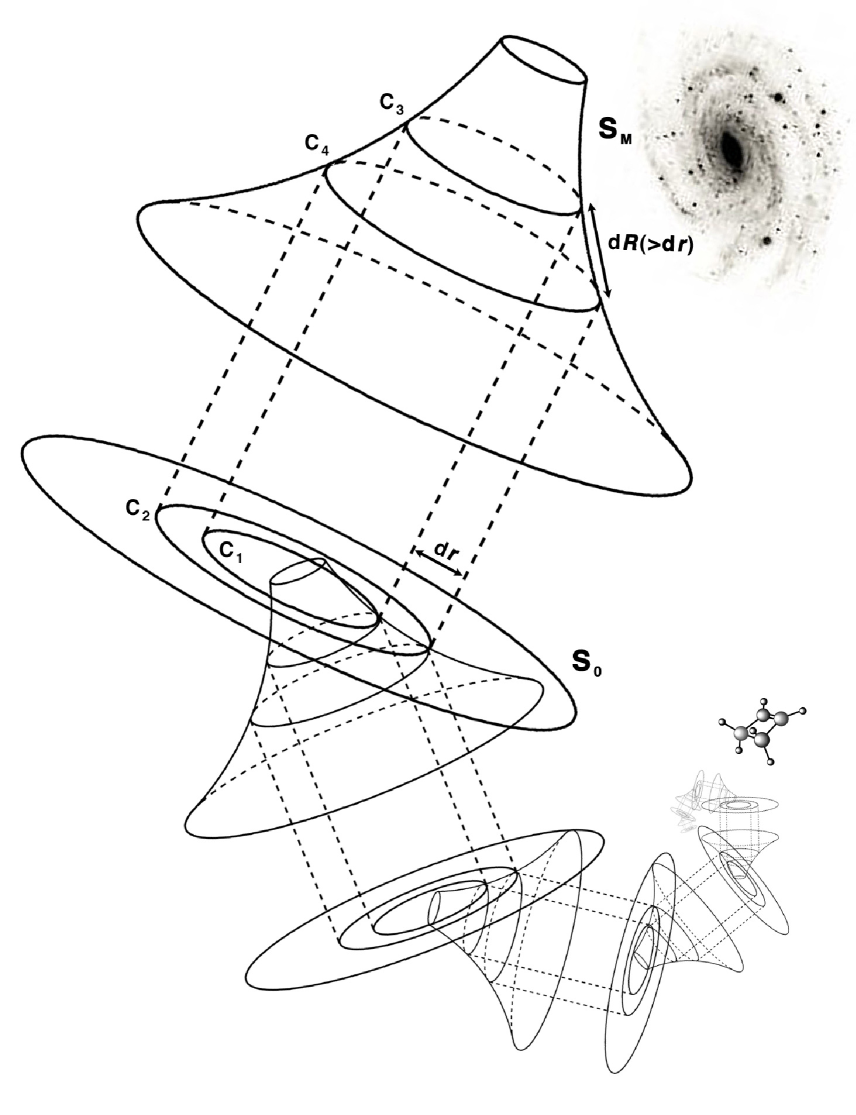
Figure 1: System of nested curved surfaces forming a spiral based on the Schwarzschild geometry due to the presence of dispersed mass (c.f., Eq.(Probability of stochastic processes and spacetime geometry)) along distance scales from the macro- to the micro-world.

References

- (1) R. Goodman in ”Introduction to Stochastic Models” (Benjamin-Cumming Publ. Comp., California, USA, 1988).
- (2) R.M. Nisbet and W.S.C. Gurney in ”Modelling Fluctuating Polpulations” (J. Wiley & Sons, NY, USA, 1982).
- (3) S. Saunders, in ”Chance in Physics: Foundations and Perspectives” (J. Bricmont et al. Eds., Springer-Verlag, 2001).
- (4) J. Foster and J.D. Nightingale in ”A Short Course in General Relativity” (Springer-Verlag, NY, USA, 1994).
- (5) R. Penrose, in ”The emperor’s new mind: concerning computers, minds, and the laws of physics.” (Oxford University Press, NY, USA, 1989).
- (6) J.D. Bekenstein, preprint arXiv:gr-qc/9710076 v2 (1998).
- (7) G.E.A. Matsas, Brazilian J. Phys. 34 (2004) No.1A.
- (8) S.W. Hawking, in ”A brief history of time: from the big bang to black holes” (Bantam Books, Toronto, Canada, 1988).
- (9) D. Stauffer and C. Schulze, preprint arXiv:phyics/0503101 (2005).
- (10) M. Ausloos, P. Clippe, J. Miśkieiwicz and A. Pekalski, Phys. A 344 (2004) 1.
- (11) A.Y. Menshutin and L.N. Shchur, Phys. Rev. E 73 (2006) 011407.
- (12) C.R. Doering, K.V. Sargsyan and L.M. Sander, preprint arXiv:q-bio.PE/0401016 (2004).
- (13) G.F.R. Ellis and T. Buchert, Phys. Lett. A 347 (2005) 38.
- (14) E. Minguzzi, Am. J. Phys. 73 (2005) 1117.
- (15) W.P. Tarkowski, Class. Quant. Grav. 18 (2001) 2359. See also preprint arXiv:gr-qc/0407070 (2004).
- (16) U. Seifert, J. Phys. A: Math. Gen 37 (2004) L517.
- (17) C. Jarzynski, J. Phys. A: Math. Gen 38 (2005) L227.
- (18) J.F. Beacom, preprint arXiv:astro-ph/0602101 (2006).
- (19) A.S. Novozhilov, G.P. Karev and E.V. Koonin, Briefings in BioInformatics 7 (2006) 70.
- (20) P. Gaspard, Physica A 263 (1999) 315.
- (21) G.F.R. Ellis and T. Buchert, Phys. Lett. A 347 (2005) 38.
- (22) L. J. Curtis and D.G. Ellis, Eur. J. Phys 27 (2006) 485.