On the parabolic equation method in internal wave propagation

Abstract

A parabolic equation for the propagation of periodic internal waves over varying bottom topography is derived using the multiple-scale perturbation method. Some computational aspects of the numerical implementation are discussed. The results of numerical experiments on propagation of an incident plane wave over a circular-type shoal are presented in comparison with the analytical result, based on Born approximation.

,  and

1 Introduction

The parabolic equation method, as an approximation to some elliptic problems, has been extensively used in mathematical physics. It was introduced by Leontovich & Fock [1] in the theory of electromagnetic wave propagation, applied in monograph of Babich & Buldyrev [2] to various diffraction problems and developed by Tappert [3] and his successors in underwater acoustics. Later it appeared also in the theory of surface water wave propagation in works of Liu & Mei [4], Radder [5], Kirby & Dalrymple [6] and others. Since then, it has been proven through the contribution of several authors to be an effective model for dealing rapidly and accurately with propagation problems in coastal areas.

The standard, or narrow angle parabolic wave equation has the form of the quantum mechanical non-stationary Schrödinger equation and describes the propagation of waves in weakly inhomogeneous media, at small angles with a preferred direction (taken to be in this paper the $x$-direction). Being of the evolution type equation, it can be solved in the frame of the initial-boundary value problems and has an advantage over the geometric optic method in describing the wave field near a caustic. In the theory of the surface water wave propagation the parabolic equation method now can be considered as classic and is well explained in Mei’s monograph [7]. In this theory some more complicated models, which describe wide-angle propagation [8] and include some nonlinear effects [6, 9], were also developed.

In the theory of internal wave propagation, though the geometric optic method is well-developed [10, 11, 12], little is known about the parabolic equation method, except the Kadomtsev-Petviashvili equation, which in the variable topography case was derived for the interfacial waves in [13].

The case of continuous stratification is in close analogy with the acoustic case, where the adiabatic mode parabolic equations were first derived by the factorization method in [14] and later by the multiple-scale method in [15] and [16].

The aim of our work is to obtain a standard parabolic equation for the internal wave propagation in the most simple cases and briefly discuss related computational aspects. Rotation, which is ignored at this stage, can be included in the model as weak rotation [13], and will be considered in our further publications.

As an illustration we present some numerical calculations performed in the case of refraction of an incident plane wave on a circular-like shoal.

2 Formulation and scaling

The system of linear equations, describing small amplitude motions of stratified inviscid fluid with harmonic dependence on time $t$ by the factor $e^{-\mathrm{i}\omega t}$, from which we are starting, is

$$\begin{split}-\mathrm{i}\omega\rho_{0}u+P_{x}=0\\ -\mathrm{i}\omega\rho_{0}v+P_{y}=0\\ -\mathrm{i}\omega\rho_{0}w+P_{z}+g\rho_{1}=0\\ -\mathrm{i}\omega\rho_{1}+w\rho_{0z}=0\\ u_{x}+v_{y}+w_{z}=0\end{split}$$ (1)

Here $x$, $y$, and $z$ are the Cartesian coordinates (vertical axis is directed upward), $\rho_{0}=\rho_{0}(z)$ is the undisturbed density, $P$ is the pressure, $g$ is the gravity acceleration, $\rho_{1}=\rho_{1}(x,y,z)$ is the perturbation of density due to motion, and $u$, $v$ and $w$ are respectively the $x$, $y$ and $z$ components of velocity.

We consider these equations with the boundary conditions

$$\begin{split}w=0\quad&\mbox{at}\quad z=0\\ w+uH_{x}+vH_{y}=0\quad&\mbox{at}\quad z=-H\end{split}$$ (2)

where $H=H(x,y)$ is the bottom depth.

To begin the multiple-scale procedure [17], we introduce a small parameter $\epsilon$, the slow variables $X=\epsilon x$ and $Y=\epsilon^{1/2}y$, the fast variable $\xi=(1/\epsilon)\Theta(X,Y)$ and expand the dependent variables as follows:

$$u=u_{0}+\epsilon u_{1}+\ldots\mbox{,\qquad}v=\epsilon^{1/2}v_{1/2}+\ldots\mbox{,}$$

$$w=w_{0}+\epsilon w_{1}+\ldots\mbox{,\qquad}P=P_{0}+\epsilon P_{1}+\ldots$$

The scaling used in the definition of the slow variables is characteristic for the parabolic equation method [1, 7, Section 4.10], with $x$-direction as the principal propagation direction and $y$-direction as the transverse direction.

From now on we assume that

$$H=H_{0}(X)+\epsilon H_{1}(X,Y)\,,$$

so $H_{0}$ is independent of $Y$.

We also expand $\rho_{1}$ in powers of $\epsilon$

$$\rho_{1}=\rho_{10}+\epsilon\rho_{11}+\ldots\,.$$

Substitution of these expansions into system (1) and the boundary conditions (2) and changing the partial derivatives for the prolonged ones by the rules

$$\begin{split}&\frac{\partial}{\partial x}\rightarrow\epsilon\frac{\partial}{\partial X}+\Theta_{X}\frac{\partial}{\partial\xi}\,,\\ &\frac{\partial}{\partial y}\rightarrow\epsilon^{1/2}\frac{\partial}{\partial Y}+\Theta_{Y}\frac{\partial}{\partial\xi}\,,\end{split}$$

leads to the system of equations

$$-\mathrm{i}\omega\rho_{0}(u_{0}+\epsilon u_{1}+\ldots)+\epsilon(\frac{\partial}{\partial X}+\frac{1}{\epsilon}\Theta_{X}\frac{\partial}{\partial\xi})(P_{0}+\epsilon P_{1}+\ldots)=0 \,,$$ (3)

$$-\mathrm{i}\omega\rho_{0}(\epsilon^{1/2}v_{1/2}+\ldots)+\epsilon^{1/2}(\frac{\partial}{\partial Y}+\frac{1}{\epsilon}\Theta_{Y}\frac{\partial}{\partial\xi})(P_{0}+\epsilon P_{1}+\ldots)=0 \,,$$ (4)

$$-\mathrm{i}\omega\rho_{0}(w_{0}+\epsilon w_{1}+\ldots)+P_{0z}+\epsilon P_{1z}+\ldots+g(\rho_{10}+\epsilon\rho_{11}+\ldots)=0 \,,$$ (5)

$$-\mathrm{i}\omega(\rho_{10}+\epsilon\rho_{11}+\ldots)+(w_{0}+\epsilon w_{1}+\ldots)\rho_{0z}=0 \,,$$ (6)

$$\begin{split}\epsilon(\frac{\partial}{\partial X}+\frac{1}{\epsilon}&\Theta_{X}\frac{\partial}{\partial\xi})(u_{0}+\epsilon u_{1}+\ldots)\\ +&\epsilon^{1/2}(\frac{\partial}{\partial Y}+\frac{1}{\epsilon}\Theta_{Y}\frac{\partial}{\partial\xi})(\epsilon^{1/2}v_{1/2}+\ldots)+w_{0z}+\epsilon w_{1z}+\ldots=0\,,\end{split}$$ (7)

with the boundary conditions

$$w_{0}+\epsilon w_{1}+\ldots=0\qquad\text{at}\quad z=0\,,$$ (8)

$$\begin{split}w_{0}+&\epsilon w_{1}+\ldots+\epsilon(u_{0}+\epsilon u_{1}+\ldots)\frac{\partial}{\partial X}(H_{0}+\epsilon H_{1})\\ &+\epsilon^{1/2}(\epsilon^{1/2}v_{1/2}+\ldots)\frac{\partial}{\partial Y}(H_{0}+\epsilon H_{1})=0\qquad\text{at}\quad z=-(H_{0}+\epsilon H_{1})\,.\end{split}$$ (9)

3 The parabolic equation

Equating coefficients in Eqs. (3-9) of like powers of $\epsilon$, we obtain equations describing $u_{l},w_{l},v_{l+1/2}$, $l=0,1,\ldots$.

At the order $-1/2$ in $\epsilon$ we obtain from (4)

$$\Theta_{Y}P_{0\xi}=0\,,$$

and put $\Theta_{Y}=0$, so in the sequel $\Theta$ depends only on $X$, $\Theta=\Theta(X)$.

At the zeroth order in $\epsilon$ we have

$$-\mathrm{i}\omega\rho_{0}u_{0}+\Theta_{X}P_{0\xi}=0\,,$$ (10)

$$-\mathrm{i}\omega\rho_{0}w_{0}+P_{0z}=-g\rho_{10}\,,$$ (11)

$$-\mathrm{i}\omega\rho_{10}+w_{0}\rho_{0z}=0\,,$$ (12)

$$\Theta_{X}u_{0\xi}+w_{0z}=0\,,$$ (13)

with the boundary conditions

$$\begin{split}w_{0}=0\quad&\mbox{at}\quad z=0\,,\\ w_{0}=0\quad&\mbox{at}\quad z=-H_{0}\,.\end{split}$$

After substitution in Eq. (11) $\rho_{10}$ from Eq. (12) we get

$$(\omega^{2}\rho_{0}+g\rho_{0z})w_{0}+\mathrm{i}\omega P_{0z}=0\,.$$ (14)

Twice differentiating this equation with respect to $\xi$ and using the expression

$$P_{0z\xi\xi}=-\frac{1}{(\Theta_{X})^{2}}\mathrm{i}\omega(\rho_{0}w_{0z})_{z},$$

obtained from Eqs. (10) and (13), we get

$$(\Theta_{X})^{2}(\omega^{2}\rho_{0}+g\rho_{0z})w_{0\xi\xi}+\omega^{2}(\rho_{0z}w_{0z})_{z}=0\,.$$

We seek a solution of this equation in the form of WKB-type anzatz $w_{0}=A(X,Y)\phi(X,z)e^{i\xi}$, where $\phi$ is an eigenfunction with the eigenvalue $k^{2}=(\Theta_{X})^{2}$ of the spectral problem

$$\begin{split}&\omega^{2}(\rho_{0}\phi_{z})_{z}-k^{2}(\omega^{2}\rho_{0}+g\rho_{0z})\phi=0\,,\\ &\phi(0)=\phi(-H_{0})=0\,,\end{split}$$ (15)

normalized by the condition

$$\frac{\omega^{2}}{k^{2}}\int^{0}_{-H_{0}}\rho_{0}\cdot(\phi_{z})^{2}dz=-\int^{0}_{-H_{0}}(\omega^{2}\rho_{0}+g\rho_{0z})\phi^{2}dz=1\,.$$ (16)

This problem is known as the main spectral problem of the linear internal wave theory.

At $O(\epsilon^{1/2})$ we have only one equation

$$-\mathrm{i}\omega\rho_{0}v_{1/2}+P_{0Y}=0\,,$$ (17)

which express the balance in the transverse direction for the quantities of order $<O(\epsilon)$.

The system of equations at the first order in $\epsilon$ is

$$-\mathrm{i}\omega\rho_{0}u_{1}+\Theta_{X}P_{1\xi}+P_{0X}=0\,,$$ (18)

$$-\mathrm{i}\omega\rho_{0}w_{1}+P_{1z}=-g\rho_{11}\,,$$ (19)

$$u_{0X}+\Theta_{X}u_{1\xi}+v_{1/2Y}+w_{1z}=0\,,$$ (20)

$$-\mathrm{i}\omega\rho_{11}+w_{1}\rho_{0z}=0\,,$$ (21)

with the boundary conditions

$$w_{1}=0\qquad\mbox{at}\qquad z=0\,,$$ (22)

and

$$w_{0}(z)+\epsilon w_{1}(z)+\epsilon u_{0}(z)H_{0X}=0\qquad\mbox{at}\qquad z=-H_{0}-\epsilon H_{1}\,.$$

Expanding velocities in Taylor series with respect to $z$ at $z=-H_{0}$ and collecting terms at $\epsilon^{1}$, we reduce the last boundary condition on $z=-H_{0}$

$$w_{1}-w_{0z}H_{1}+u_{0}H_{0X}=0\qquad\mbox{at}\qquad z=-H_{0}\,.$$ (23)

Considerations, similar to those in the derivation of the spectral problem Eq. (15) (the details are given in Appendix A), lead at $O(\epsilon)$ to the equation

$$\begin{split}(\omega^{2}\rho_{0}+g\rho_{0z})w_{1\xi\xi}+&\frac{\omega^{2}}{k^{2}}(\rho_{0}w_{1z})_{z}\\ &=-\frac{\omega^{2}}{k^{2}}\left(2(\rho_{0}u_{0X})_{z}+\frac{1}{\mathrm{i}\omega}P_{0YYz}-\frac{k_{X}}{k}(\rho_{0}u_{0})_{z}\right)\,.\end{split}$$ (24)

Seeking solutions of Eq. (24) which depend on $\xi$ by the factor $\exp(\mathrm{i}\xi)$, we obtain for $w_{1}$ the equation

$$\begin{split}\omega^{2}(\rho_{0}w_{1z})_{z}-k^{2}(\omega^{2}\rho_{0}+&g\rho_{0z})w_{1}\\ &=-\omega^{2}\left(2(\rho_{0}u_{0X})_{z}+\frac{1}{\mathrm{i}\omega}P_{0YYz}-\frac{k_{X}}{k}(\rho_{0}u_{0})_{z}\right)\,.\end{split}$$ (25)

A solution to this differential equation with respect to $z$ with the boundary conditions Eqs. (22) and (23) can be found only when a certain compatibility condition is satisfied, because the right hand side of Eqs. (25) and (23) contain the solution of the spectral problem (15). The compatibility condition yields the required evolution equation for the amplitude function $A$

$$\begin{split}A_{X}+\frac{1}{2\mathrm{i}k}A_{YY}-\frac{1}{2}\frac{k_{X}}{k}A&+\frac{\omega^{2}}{2k^{2}}\rho_{0}(-H_{0})\cdot H_{0X}\cdot\left(\phi_{z}(X,-H_{0})\right)^{2}A\\ &-\frac{\omega^{2}}{2\mathrm{i}k}\rho_{0}(-H_{0})\cdot H_{1}\cdot\left(\phi_{z}(X,-H_{0})\right)^{2}A=0\,,\end{split}$$ (26)

which we call the parabolic equation for periodic internal waves. Rewritten in the initial coordinates $(x,y)$, it has the form

$$\begin{split}A_{x}+\frac{1}{2\mathrm{i}k}A_{yy}-\frac{1}{2}\frac{k_{x}}{k}A&+\frac{\omega^{2}}{2k^{2}}\rho_{0}(-H_{0})\cdot H_{0x}\cdot\left(\phi_{z}(x,-H_{0})\right)^{2}A\\ &-\frac{\omega^{2}}{2\mathrm{i}k}\rho_{0}(-H_{0})\cdot\bar{H}_{1}\cdot\left(\phi_{z}(x,-H_{0})\right)^{2}A=0\,,\end{split}$$ (27)

where $\bar{H}_{1}(x,y)=\epsilon H_{1}(\epsilon x,\epsilon^{1/2}y)$, For detailed derivation of Eq. (26) see Appendix B.

For the numerical calculation of the coefficients of Eq. (26) can be used, in principle, any algorithm for solving the spectral problem Eq. (15). Some problems arise with the derivatives, namely, $k_{X}$ and $\phi_{z}(X,-H_{0}))$.

To avoid numerical differentiation in the calculation of $k_{X}$ we differentiate the spectral problem Eq. (15) with respect to $X$ and get the boundary value problem for $\phi_{X}$

$$\begin{split}&\omega^{2}(\rho_{0}\phi_{Xz})_{z}-k^{2}(\omega^{2}\rho_{0}+g\rho_{0z})\phi_{X}-2kk_{X}(\omega^{2}\rho_{0}+g\rho_{0z})\phi=0\,,\\ &\phi_{X}(X,0)=0\,,\qquad\phi_{X}(X,-H_{0})-H_{0X}\phi_{z}(X,-H_{0})=0\,.\end{split}$$

The compatibility condition for this problem is

$$\frac{k_{X}}{k}=-\frac{\omega^{2}}{2k^{2}}\rho_{0}(-H_{0})\cdot H_{0X}\cdot\left(\phi_{z}(X,-H_{0})\right)^{2}\,.$$

which gives the stable formula for the numerical calculation of $k_{X}/k$ (modulo the calculation of $\phi_{z}(X,-H_{0}))$).

Now we derive a formula for the stable calculation of the derivative $\phi_{z}(X,-H_{0})$. To do this, we multiply Eq. (15) by $z$ and integrate from $-H_{0}$ to zero. After integrating by parts and some transformations we get the required formula

$$\phi_{z}(X,-H_{0})=\frac{1}{\rho_{0}(-H_{0})H_{0}}\left(\frac{k^{2}}{\omega^{2}}\int^{0}_{-H_{0}}(\omega^{2}\rho_{0}+g\rho_{0z})\phi\cdot z\,dz-\int^{0}_{-H_{0}}\rho_{0z}\phi\,dz\right)\,.$$

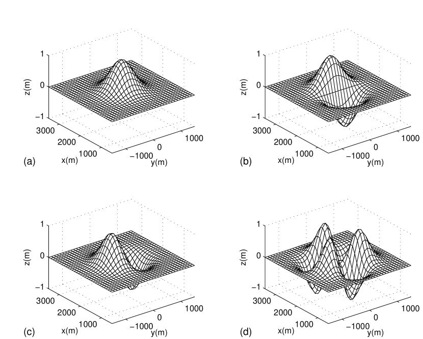
Figure 1: Bottom topography forms of the compact inhomogeneities (30) used for the numerical simulation. For all cases $h_{1}=1\,\text{m}$, $\sigma=500\,\text{m}$. (a) $M=0$, $\alpha_{0}=0$; (b) $M=1$, $\alpha_{0}=0$; (c) $M=1$, $\alpha_{0}=\pi/2$; (d) $M=3$, $\alpha_{0}=0$.

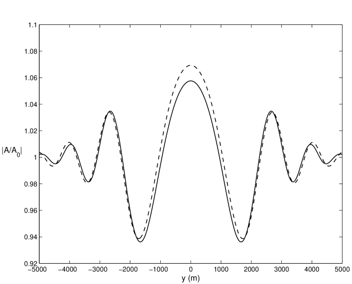
Figure 2: Transverse cross-sections at $x=12000\,\text{m}$ of relative wave field amplitudes in scattering of the 2nd mode internal waves on the shoal (30) with parameters $M=0,\sigma=500~{}m,\alpha_{0}=0$ (Fig. 1(a)). —, the parabolic equation method; - - - , the Born approximation (31).

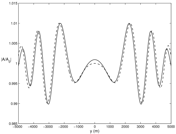
Figure 3: Transverse cross-sections at $x=12000\,\text{m}$ of relative wave field amplitudes in scattering of the 2nd mode internal waves on the shoal (30) with parameters $M=1,\sigma=500~{}m,\alpha_{0}=0$ (Fig. 1(b)). —, the parabolic equation method; - - - , the Born approximation (31).

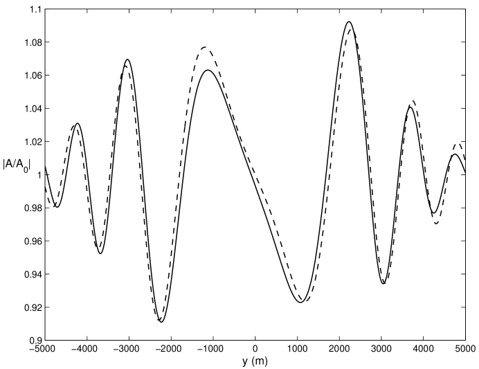
Figure 4: Transverse cross-sections at $x=12000\,\text{m}$ of relative wave field amplitudes in scattering of the 2nd mode internal waves on the shoal (30) with parameters $M=1,\sigma=500~{}m,\alpha_{0}=\pi/2$ (Fig. 1(c)). —, the parabolic equation method; - - - , the Born approximation (31).

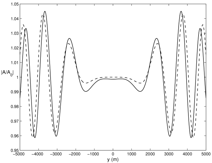
Figure 5: Transverse cross-sections at $x=12000\,\text{m}$ of relative wave field amplitudes in scattering of the 2nd mode internal waves on the shoal (30) with parameters $M=3,\sigma=500~{}m,\alpha_{0}=0$ (Fig. 1(d)). —, the parabolic equation method; - - - , the Born approximation (31).

4 Numerical experiments

The numerical experiments were conducted for a fluid with an exponential density stratification $\rho=\exp(-\gamma z)$, where $\gamma>0$. In this case the complete set of normalized solutions of the spectral problem Eq. (15) is

$$\begin{split}k_{n}=\frac{\omega}{2H_{0}}\sqrt{\frac{\gamma^{2}H_{0}^{2}+4n^{2}\pi^{2}}{g\gamma-\omega^{2}}}\,,\quad n=1,\ldots\,,\\ \phi_{n}(z)=C\exp(\gamma z/2)\sin(n\pi z/H_{0})\,,\quad n=1,\ldots\,,\end{split}$$ (28)

where $C$ is the normalizing constant

$$C=\sqrt{\frac{2}{H_{0}(g\gamma-\omega^{2})}}\,.$$ (29)

From Eqs. (28) and (29) we have also

$$\phi_{nz}(-H_{0})=(-1)^{n}C\frac{n\pi}{H_{0}}\exp(-\gamma H_{0}/2)\,.$$

For the numerical experiments the problem of the scattering of the incident plane wave of a given mode on the localized small inhomogeneities of the bottom topography was considered. So $H_{0}$ is taken to be a constant and $\bar{H}_{1}(x,y)$ describes the inhomogeneity, the total depth is $H_{0}+\bar{H}_{1}(x,y)$. For the inhomogeneities of the form

$$\bar{H}_{1}(r,\alpha)=-A_{M}r^{M}\cos(M(\alpha+\alpha_{0}))\exp(-r^{2}/\sigma^{2})\,,M=1,\ldots\,,$$ (30)

where $(r,\alpha)$ are the polar coordinates centered at the point $(x_{0},y_{0}=0)$ with $\alpha=0$ corresponding to the positive $x$-direction, the scattering problem for the propagating in $x$-direction incident plane wave of the $n$th mode with the vertical velocity $w_{inc}=A_{0}\exp(\mathrm{i}k_{n}(x-x_{0}))\phi_{n}$ admits an approximate solution in which the $n$th mode component of the scattered field is

$$\begin{split}w_{n}^{scat}(r,\alpha,z)=&A_{n}(r,\alpha)\phi_{n}=\left(A_{0}A_{M}G\,\mathrm{i}^{M+1}\,\sqrt{\frac{\pi}{2}}\,\frac{\kappa^{M}\sigma^{2M+2}}{2^{M+1}}\frac{e^{\mathrm{i}(k_{n}r-\pi/4)}}{\sqrt{k_{n}r}}\right.\\ &\left.\times\exp(-\frac{\sigma^{2}(k^{2}_{n}-k^{2}_{n}\cos\alpha)}{2})\cos M(\psi-\alpha_{0})\cos\alpha\right)\cdot\phi_{n}\,,\\ \end{split}$$ (31)

where $G=\omega^{2}\rho(-H_{0})\left(\phi_{nz}(-H_{0})\right)^{2}$, $\kappa=\sqrt{2k^{2}_{n}-2k^{2}_{n}\cos\alpha}$  and $\tan(\psi)=\sin\alpha/(1-\cos\alpha)$. The quantity that will be compared with the solution of the parabolic equation (27) is the absolute value of the $n$th mode part amplitude of the incident$+\,$scattered field

$$|A(x,y)|=|A_{0}\exp(\mathrm{i}k_{n}(x-x_{0}))+A_{n}(\sqrt{(x-x_{0})^{2}+y^{2}},\arctan(y/(x-x_{0})))|\,.$$

The solution Eq. (31) was obtained by the methods of the work [18] in the frame of the Born and far field approximations. The methods of the work [18] do not use any assumptions on the preferred propagation direction and are closely related to the methods of the work [19].

The numerical experiments were conducted on the computational domain $[0\leq x\leq 12000]\times[-5000\leq y\leq 5000]$, where $x$ and $y$ are measured in meters. Eq. (27) with the initial condition $A_{0}=A(0,y)=constant$ was integrated on the grid $395\times 349$ by the Crank-Nicholson scheme [20]. In order to exclude reflections at the boundaries, the absorbing Baskakov-Popov boundary conditions were used [21], which were adapted for non-vanishing at the boundaries initial conditions.

The inhomogeneities in all cases have width parameter $\sigma=500\,\mbox{m}$ and the amplitude $h_{1}=A_{M}\exp(-M/2)\left(\sigma\sqrt{M/2}\,\right)^{M}=1\,\text{m}$ with the center positioned at $x_{0}=2000\,\mbox{m}$, $y_{0}=0\,\mbox{m}$. The shape parameters $M$ and $\alpha_{0}$ were varied (see Fig. 1). The depth of the flat bottom, $H_{0}$, was taken to be 60 m. The density stratification parameter $\gamma=0.00025$, which corresponds to the Brunt-Väisälä frequency $N=\sqrt{g\gamma}\approx 0.05\,s^{-1}$.

The computations were done for the 1st mode and 2nd mode incident plane waves with 15 min time period. The transverse cross-sections of the 2nd mode computed field amplitude at $x=12000~{}\text{m}$ are presented in Fig. 2-5 in comparison with the Born type approximation scattering results obtained by Eq. (31). The results for the 1st mode are analogous.

Considering the results of computations, it is worth noting that the solution (31) has an approximative character, so the comparison with it is not exactly the test of accuracy of the derived parabolic equation. Nevertheless, since Eq. (31) is of quite different genesis, and, in particular, free from any assumptions on the preferred propagation direction, this comparison can lead to the conclusion that the parabolic equation describes sufficiently well the waves with propagation angles up to $45^{\,\circ}$ (see the discussion on the propagation angles in [8]), scattering on the enough rough topography.

5 Conclusion

For the propagation of periodic internal waves over uneven bottom topography with small irregularities, the narrow-angle parabolic equation (27) has been derived. It also takes into account slow, but not necessary small, variations of bottom topography in principal propagation direction.

We have illustrated the use of the obtained equation by presenting the results of scattering of the plane internal waves over shoals of the special forms (30). The results of computations are in a sufficiently good agreement with the analytical solution (31), obtained in the frame of the Born approximation, and support the applicability of equation (27) for computing of internal wave fields over uneven bottom with restrictions typical for the parabolic equation method in general [3, 7].

Appendix A Derivation of Eq. (24)

From (19, 21) we obtain

$$(\omega^{2}\rho_{0}+g\rho_{0z})w_{1}+\mathrm{i}\omega P_{1z}=0\,.$$ (32)

From (18) we get

$$P_{1\xi\xi}=\frac{1}{\Theta_{X}}\mathrm{i}\omega\rho_{0}u_{1\xi}-\frac{1}{\Theta_{X}}P_{0X\xi}\,.$$ (33)

From (20), taking into account (17), we have

$$u_{1\xi}=-\frac{1}{\Theta_{X}}(u_{0X}+v_{1/2Y}+w_{1z})=-\frac{1}{\Theta_{X}}(u_{0X}+\frac{1}{\mathrm{i}\omega\rho_{0}}P_{0YY}+w_{1z})\,.$$ (34)

From (10) we get

$$P_{0X\xi}=\mathrm{i}\omega\left(\frac{1}{\Theta_{X}}\rho_{0}u_{0}\right)_{X}=-\mathrm{i}\omega\frac{k_{X}}{k^{2}}\rho_{0}u_{0}+\mathrm{i}\omega\frac{1}{k}\rho_{0}u_{0X}\,.$$ (35)

Substitution of $u_{1\xi}$ and $P_{0X\xi}$ from Eqs. (34, 35) into Eq. (33) gives

$$\begin{split}P_{1\xi\xi}&=-\frac{1}{k^{2}}\mathrm{i}\omega\rho_{0}\left(u_{0X}+\frac{1}{\mathrm{i}\omega\rho_{0}}P_{0YY}+w_{1z}\right)\\ &\qquad\qquad\qquad\qquad\qquad\quad-\frac{1}{k^{2}}\left(-\mathrm{i}\omega\frac{k_{X}}{k}\rho_{0}u_{0}+\mathrm{i}\omega\rho_{0}u_{0X}\right)\\ &=-\frac{1}{k^{2}}\mathrm{i}\omega\left(2\rho_{0}u_{0X}+\frac{1}{\mathrm{i}\omega}P_{0YY}+\rho_{0}w_{1z}-\frac{k_{X}}{k}\rho_{0}u_{0}\right)\,.\end{split}$$ (36)

Differentiating Eq. (36) with respect to $z$ and substituting the result into the second $\xi$-derivative of Eq. (32), we obtain Eq. (24).

Appendix B Derivation of the compatibility condition

In this appendix the compatibility condition for the boundary value problem Eqs. (25, 22 and 23) is derived.

From Eq. (14) we have

$$\frac{1}{\mathrm{i}\omega}P_{0YYz}=\frac{1}{\omega^{2}}(\omega^{2}\rho_{0}+g\rho_{0z})w_{0YY}\,.$$

From Eq. (13), taking into account that $u_{0}$ and $w_{0}$ depend on $\xi$ by the factor $e^{\mathrm{i}\xi}$, we have

$$\mathrm{i}u_{0}=-\frac{1}{k}w_{0z},\quad\mbox{or}\quad u_{0}=\frac{\mathrm{i}}{k}w_{0z}\,.$$

Substitution of these expressions into the right hand side of (25) (denote it by $RHS$) yields

$$\begin{split}RHS=&-\omega^{2}\cdot\left[\vphantom{\frac{\mathrm{i}k_{X}}{k^{2}}}2\frac{\mathrm{i}}{k}(\rho_{0}w_{0zX})_{z}-2\frac{\mathrm{i}}{k^{2}}k_{X}(\rho_{0}w_{0z})_{z}+\frac{1}{\omega^{2}}\left(\omega^{2}\rho_{0}+g\rho_{0z}\right)w_{0YY}\right.\\ &-\left.\frac{\mathrm{i}k_{X}}{k^{2}}(\rho_{0}w_{0z})_{z}\right]=-\omega^{2}\cdot\left[\vphantom{\frac{\mathrm{i}k_{X}}{k^{2}}}2\frac{\mathrm{i}}{k}A_{X}(\rho_{0}\phi_{z})_{z}+2\frac{\mathrm{i}}{k}A(\rho_{0}\phi_{Xz})_{z}\right.\\ &\left.+\frac{1}{\omega^{2}}\left(\omega^{2}\rho_{0}+g\rho_{0z}\right)A_{YY}\phi-3\frac{\mathrm{i}k_{X}}{k^{2}}A(\rho_{0}\phi_{z})_{z}\right]\cdot\exp(\mathrm{i}\xi)\,.\end{split}$$ (37)

To obtain the required compatibility condition we multiply Eq. (25) by the eigenfunction $\phi$ and integrate with respect to $z$ from $-H_{0}$ to $0$. Then twice integrating by parts Eq. (25) using Eqs. (22, 23) we obtain

$$\int^{0}_{-H_{0}}RHS\cdot\phi\,dz=\omega^{2}\rho_{0}(-H_{0})a\phi_{z}(X,-H_{0})\,,$$ (38)

where

$$\begin{split}a=&w_{1}(X,-H_{0})=w_{0z}(X,-H_{0})\cdot H_{1}-u_{0}(X,-H_{0})\cdot H_{0X}\\ &=(H_{1}-\frac{\mathrm{i}}{k}H_{0X})w_{0z}(X,-H_{0})=(H_{1}-\frac{\mathrm{i}}{k}H_{0X})A\phi_{z}(X,-H_{0})\cdot\exp(\mathrm{i}\xi)\,.\end{split}$$

From Eq. (37) and Eq. (38) we get

$$\begin{split}&2\frac{\mathrm{i}}{k}A_{X}\int^{0}_{-H_{0}}(\rho_{0}\phi_{z})_{z}\phi\,dz+\frac{1}{\omega^{2}}A_{YY}\int^{0}_{-H_{0}}(\omega^{2}\rho_{0}+g\rho_{0z})\phi^{2}dz\\ &-3\mathrm{i}\frac{k_{X}}{k^{2}}A\int^{0}_{-H_{0}}(\rho_{0}\phi_{z})_{z}\phi dz+\frac{\mathrm{i}}{k}A\int^{0}_{-H_{0}}2(\rho_{0}\phi_{Xz})_{z}\phi\,dz\\ &\qquad\qquad\qquad\qquad\quad=-\rho_{0}(-H_{0})\cdot(H_{1}-\frac{\mathrm{i}}{k}H_{0X})A\cdot\left(\phi_{z}(X,-H_{0})\right)^{2}\,.\end{split}$$ (39)

Using the normalizing condition Eq. (16) we have

$$\begin{split}&\left(\frac{\omega^{2}}{k^{2}}\int^{0}_{-H_{0}}\rho_{0}(\phi_{z})^{2}\,dz\right)_{X}\\ &=-2\frac{k_{X}}{k}+\frac{\omega^{2}}{k^{2}}\int^{0}_{-H_{0}}2\rho_{0}\phi_{z}\phi_{Xz}\,dz-\rho_{0}(-H_{0})\cdot\left(\phi_{z}(X,-H_{0})\right)^{2}H_{0X}\frac{\omega^{2}}{k^{2}}=0\,,\end{split}$$

and thus

$$\begin{split}\frac{\mathrm{i}}{k}A\int^{0}_{-H_{0}}2(\rho_{0}\phi_{Xz})_{z}\phi\,dz&=-\frac{\mathrm{i}}{k}A\int^{0}_{-H_{0}}2\rho_{0}\phi_{Xz}\phi_{z}\,dz\\ &=-\frac{\mathrm{i}}{k}A\rho_{0}(-H_{0})\cdot\left(\phi_{z}(X,-H_{0})\right)^{2}H_{0X}-2\mathrm{i}\frac{k_{X}}{\omega^{2}}A\,.\end{split}$$

With this and the normalizing condition Eq. (16) we obtain from Eq. (39) the required parabolic equation

$$\begin{split}A_{X}+\frac{1}{2\mathrm{i}k}A_{YY}-\frac{1}{2}\frac{k_{X}}{k}A&+\frac{\omega^{2}}{2k^{2}}\rho_{0}(-H_{0})\cdot H_{0X}\cdot\left(\phi_{z}(X,-H_{0})\right)^{2}A\\ &-\frac{\omega^{2}}{2\mathrm{i}k}\rho_{0}(-H_{0})\cdot H_{1}\cdot\left(\phi_{z}(X,-H_{0})\right)^{2}A=0\,.\end{split}$$

References

[1]
Leontovich, M. A., Fock, V. A., 1965. Solution of the problem of
propagation of electromagnetic waves along the Earth’s surface by
the method of parabolic equations. Chapter 11, Electromagnetic
Diffraction and Propagation Problems, ed. V. A. Fock. Pergamon
Press.
[2]
Babich, V. M., Buldyrev, V. S., 1972. Asymptotic methods in problems
of short-wave diffraction. Nauka, Moscow. (In Russian).
[3]
Tappert, F. D., 1977. The parabolic approximation method, in Wave
Propagation and Underwater Acoustics, ed. J. B. Keller,
J. S. Papadakis. Lecture Notes in Physics, Springer-Verlag, Berlin
and New-York.
[4]
Liu, P. L. F., Mei, C. C., 1976. Water motion on a beach in the
presence of a breakwater. 1. J. Geoph. Res. 81, 3079-3094.
[5]
Radder, A. C., 1979. On the parabolic equation method for
water-wave propagation. J. Fluid Mech. 95, 159-176.
[6]
Kirby, J. T., Dalrymple, R. A., 1983. A parabolic equation for the
combined refraction-diffraction of Stokes waves by mildly varying
topography. J. Fluid Mech. 136, 453-466.
[7]
Mei, C. C., 1983, The applied dynamics of ocean surface waves.
John Wiley & Sons, New York et al..
[8]
Dalrymple, R. A, Kirby, J. T., 1988. Models for very wide-angle water
waves and wave diffraction. J. Fluid Mech. 192, 33-50.
[9]
Liu, P. L.-F, Yoon, S. B, 1985. Nonlinear refraction-diffraction of waves
in shallow water. J. Fluid Mech. 153, 185-201.
[10]
Keller, J. B., van Mow, C, 1969. Internal wave propagation in an inhomofeneous
fluid of non-uniform depth. J. Fluid Mech. 38, 365-374.
[11]
Miropolsky, Yu. Z., 1974. Propagation of internal waves in theocean with
horizontal inhomogeneities of the density field. Izvestiya USSR Academy
of Sciences, Physics of Atmosphere and Oceans 10(5), 519-532 (in Russian).
[12]
Voronovich, A. G., 1976. The propagation of surface and internalwaves in an
approach of geometrical optics. Izvestiya USSR Academy of Sciences,
Physics of Atmosphere and Oceans 12 (8), 850-857, (in Russian).
[13]
Chen, Y., Liu, P. L.-F., The Kadomtsev-Petviashvili equation for interfacial waves,
1995. J. Fluid Mech. 288, 383-408.
[14]
Collins, M. D., 1993. The adiabatic mode parabolic equation. J.
Acoust. Soc. Amer. 94, 2269-2278.
[15]
Trofimov, M. Yu., 1999. Narrow-Angle Parabolic Equations of
Adiabatic Single-Mode Propagation in a Horizontally Inhomogeneous
Shallow Sea. Acoust. Phys. 45, 575-580.
[17]
Nayfeh, A. H., 1973. Perturbation methods. John Wiley & Sons, New
York et al..
[18]
Zakharenko, A. D., 2002. Scattering of internal waves from small
sea bottom inhomogeneities. Proceedings of The Sixth Pan Ocean
Remote Sensing Conference (PORSEC), Bali, 3-6 September 2002,
Vol. II, pp. 773-777, arXiv:physics/0701221.
[19]
Llewellin Smith, S. G., 2002. Conversion of the barotropic tide. J.
Phys. Oceanogr. 32, 1554-1566.
[20]
Potter, D., 1973. Computational physics. John Wiley & Sons, N.-Y.
[21]
Baskakov, V. A., Popov A. V., 1991. Implementation of transparent
boundaries for numerical solution of the Schrödinger equation.
Wave Motion 14, 123-128.