MontePython: Implementing Quantum Monte Carlo using Python

Abstract

We present a cross-language C++/Python program for simulations of quantum mechanical systems with the use of Quantum Monte Carlo (QMC) methods. We describe a system for which to apply QMC, the algorithms of variational Monte Carlo and diffusion Monte Carlo and we describe how to implement theses methods in pure C++ and C++/Python. Furthermore we check the efficiency of the implementations in serial and parallel cases to show that the overhead using Python can be negligible.

I Introduction

In scientific programming there has always been a struggle between computational efficiency and programming efficiency. On one hand, we want a program to go as fast as possible, resorting to low-level programming languages like FORTRAN77 and C which can be difficult to read and even harder to debug. On the other hand, we want the programming process to be as efficient as possible, turning to high-level software like Matlab, Octave, Maple, R and S+. Here features like clean syntax, interactive command execution, integrated simulation and visualization and rich documentation make us feel more productive. However, if we have some well tested and fast routines written in low-level language, interfacing these routines with, e.g., Matlab is rather cumbersome. Most often, we will end up using similar Matlab routines, which are often written as generally as possible at the cost of computing efficiency.

Recently, the programming language Python python has emerged as a potential competitor to Matlab. Python is a very powerful programming language which, when extended with numerical and visual modules like SciPy scipy , shares many of the features of Matlab. In addition, Python was designed to be extendible with compiled code for efficiency and several tools are available for doing so.

In this paper we will demonstrate how Python can be extended with compiled code to yield an efficient scientific program. Specifically, we will start with a Monte Carlo simulator written in C++ and, with the help of SWIG swig , reuse the C++ code in a Python Monte Carlo simulator. We will show that this porting from low-level to high-level code can be achieved without significant loss of efficiency.

The remainder of this paper is organized as follows. In section II we define the system we apply the Monte Carlo simulator to. Section III discuss in some detail the algorithms we are going to use, i.e., variational Monte Carlo and diffusion Monte Carlo. Next, we go through the implementations of diffusion Monte Carlo, both in C++ and Python, in section III. Furthermore, section V compare the efficiency of C++ and Python for varying numbers of CPUs and section VII visualize the output from diffusion Monte Carlo with the use of Python. Finally, we round off with some remarks in section VIII.

II The system

Quantum Monte Carlo (QMC) has a wide range of applications, for example studies of Bose-Einstein condensates of dilute atomic gases (bosonic systems) dubois2003 and studies of so-called quantum dots (fermionic systems) harju2005 , electrons confined between layers in semi-conductors. In this paper we will focus on a model which is meant to reproduce the results from an experiment by Anderson & al. anderson . Anderson & al. cooled down $4\times 10^{6}$ ⁸⁷Rb to temperatures in the order of $100\,nK$ to observe Bose-Einstein condensation in the dilute gas. Our physical motivation in this paper is to model numerically this fascinating experiment. This should be done in an as general as possible way, so that we can expand our computations to systems not yet explored in experiments. We will in this section go through the steps needed to put the experiment into the framework of QMC.

In QMC the goal is to solve the Schrödinger equation

$$i\hbar\frac{\partial}{\partial t}\Psi(\boldsymbol{\mathbf{R}},t)=H\Psi(\boldsymbol{\mathbf{R}},t),$$ (1)

or rather the time independent version

$$H\Psi(\boldsymbol{\mathbf{R}})=E\Psi(\boldsymbol{\mathbf{R}}).$$ (2)

Thus, to model the experiment above using Quantum Monte Carlo methods, all we need is a Hamiltonian and a trial wave function. The Hamiltonian for $N$ trapped interacting atoms is given by

$$H=-\frac{\hbar^{2}}{2m}\sum_{i=1}^{N}\nabla_{i}^{2}+\sum_{i=1}^{N}V_{ext}(\boldsymbol{\mathbf{r}}_{i})+\sum_{i<j}^{N}V_{int}(|\boldsymbol{\mathbf{r}}_{i}-\boldsymbol{\mathbf{r}}_{j}|).$$ (3)

Taking advantage of the fact that the gas is dilute, we can describe the two-body interaction $V_{int}(|\boldsymbol{\mathbf{r}}_{i}-\boldsymbol{\mathbf{r}}_{j}|)$ by a hard-core potential of radius $a$, where $a$ is the scattering length, thus treating the atoms as hard spheres nilsen2005 .

We define the trial wave function by

$$\Psi_{T}=\prod_{i}g(\boldsymbol{\mathbf{r}}_{i})\prod_{i<j}f(r_{ij}),$$ (4)

where $g(\boldsymbol{\mathbf{r}}_{i})$ describes the interaction between one particle and the external potential, $V_{ext}$, while the two-body correlation function $f(r_{ij})$ describes the interaction between two particles. The function $f(r_{ij})$ is the solution of the Schrödinger equation for a pair of atoms at very low energy interacting via a hard-core potential of radius $a$. The ansatz for $f(r)$ reads

$$f(r)=\left\{\begin{array}[]{lll}\left(1-a/r\right)&&r>a\\ 0&&r\leq a.\end{array}\right.$$ (5)

Besides being physically motivated, this type of correlation has been successfully used in refs. dubois2001 and dubois2003 to study both spherically symmetric and deformed traps. In the experiment of Anderson & al., the particles were trapped in a disk-shaped harmonic oscillator potential. This corresponds to using an external potential

$$V_{ext}=\frac{m}{2}\left(\omega_{\perp}x^{2}+\omega_{\perp}y^{2}+\omega_{z}z^{2}\right)$$ (6)

If we neglect the particle-particle interaction and insert the potential of eq. (6) into eq. (2) we obtain

$$g(\boldsymbol{\mathbf{r}})=A(\alpha)\lambda^{1/4}\exp\left(-\alpha(x^{2}+y^{2}+\lambda z^{2})\right)$$ (7)

where $\alpha$ is taken as the variational parameter of the calculation and $A(\alpha)=(2\alpha/\pi)^{3/4}$ is a normalization constant. The parameter $\lambda=\omega_{z}/\omega_{\perp}$ is kept constant and set equal to the asymmetry of the trap. Still following Anderson & al. we let $\lambda=\sqrt{8}$ throughout this paper.

III The algorithms

In this section we will go through the algorithms used in this paper. First, we will discuss Monte Carlo integration in general. Second, we state the Variational Monte Carlo algorithm and last, we go through the Diffusion Monte Carlo algorithm.

III.1 Monte Carlo Integration

Monte Carlo integration is best described through conventional numerical integration methods. In conventional methods we fix the evaluation points and weights of the integrand in advance,

$$\int_{\Omega}f(\boldsymbol{\mathbf{r}})d\Omega=\sum_{i=1}^{m}\omega_{i}f(r_{i})+\mathcal{O}\left(\frac{1}{m}\right).$$ (8)

If we choose the evaluation points with equal spacing over the integration area, a two dimensional integral can for example be written as

$$\int_{0}^{1}\int_{0}^{1}f(x,y)\,dxdy=\frac{1}{m^{2}}\sum_{i=1}^{m}\sum_{i=1}^{m}f(x_{i},y_{j})\mathcal{O}\left(\frac{1}{m}\right).$$ (9)

For $N$ dimensions we have to carry out $m^{N}$ evaluations of $f(r)$ to obtain an accuracy of $\mathcal{O}\left(\frac{1}{m}\right)$. In Monte Carlo integration the integrand is evaluated at random points $\boldsymbol{\mathbf{r}}_{i}$ drawn from an arbitrary probability distribution $\rho(\boldsymbol{\mathbf{r}})$,

$$\int_{\Omega}f(\boldsymbol{\mathbf{r}})\,d\Omega=\int_{\Omega}g(\boldsymbol{\mathbf{r}})\rho(\boldsymbol{\mathbf{r}})\,d\Omega=\sum_{i=1}^{m}g(r_{i})+\mathcal{O}\left(\frac{1}{\sqrt{m}}\right).$$ (10)

The main advantage of this scheme is that it is independent of the number of dimensions of $\boldsymbol{\mathbf{R}}$. Note, however, that the efficiency of the integration depends on a good choice for $\rho(\boldsymbol{\mathbf{R}})$.

III.1.1 Metropolis Algorithm

The Metropolis Algorithm metropolis generates a stochastic sequence of phase space points that samples a given probability distribution. In Quantum Monte Carlo methods each point in phase space represents a vector $\boldsymbol{\mathbf{R}}=\{\boldsymbol{\mathbf{r}}_{1},\boldsymbol{\mathbf{r}}_{2},\ldots,\boldsymbol{\mathbf{r}}_{N}\}$ in Hilbert space. Here $\boldsymbol{\mathbf{r}}_{i}$ represents all degrees of freedom for particle $i$. Coupled with a quantum mechanical operator (like the Hamiltonian in eq. (3)) each such point can be associated with physical quantities (the Hamiltonian gives the energy of the system). The fundamental idea behind the Metropolis algorithm is that the sequence of individual samples of these quantities can be combined to arrive at average values which describes the quantum mechanical state of the system. The Metropolis algorithm provides the sample points. From an initial position in phase space a proposed move is generated and the move is either accepted or rejected according to the Metropolis algorithm

$$P_{A}(\boldsymbol{\mathbf{R}}^{\prime},\boldsymbol{\mathbf{R}})=min\left(1,\frac{\rho(\boldsymbol{\mathbf{R}}^{\prime})}{\rho(\boldsymbol{\mathbf{R}})}\right).$$ (11)

where $P_{A}(\boldsymbol{\mathbf{R}}^{\prime},\boldsymbol{\mathbf{R}})$ is the probability of moving the particle from $\boldsymbol{\mathbf{R}}$ to $\boldsymbol{\mathbf{R}}^{\prime}$. In this way a random walk generates a sequence $\{\boldsymbol{\mathbf{R}}_{0},\boldsymbol{\mathbf{R}}_{1},\ldots,\boldsymbol{\mathbf{R}}_{i},\ldots\}$ of points in phase space. It is important that all points must be accessible from any starting point; the random walk must be ergodic.

Metropolis & al. showed that the sampling is most easily achieved if the points $\boldsymbol{\mathbf{R}}$ form a Markov chain. A random walk is Markovian if each point in the chain depends only on the position of the previous point.

III.2 Variational Monte Carlo

Variational Monte Carlo (VMC) is the starting point of all Monte Carlo calculations in that we need an optimized trial wave function as input to the other Monte Carlo methods. In VMC we combine Monte Carlo integration with the Metropolis algorithm and the variational principle to get the trial wave function that yields the lowest energy.

The variational principle states that, given a variational wave function $\psi_{\alpha}$ (where $\alpha=\alpha_{1},\alpha_{2},\ldots$ denote a set of variational parameters), the energy expectation value of $\psi_{\alpha}$ provides an upper bound to the ground state energy, i.e.,

$$\langle H\rangle_{\alpha}=\frac{\int\psi_{\alpha}^{*}(\boldsymbol{\mathbf{R}})H\psi_{\alpha}(\boldsymbol{\mathbf{R}})\,d\boldsymbol{\mathbf{R}}}{\int\psi_{\alpha}^{(}\boldsymbol{\mathbf{R}})*\psi_{\alpha}(\boldsymbol{\mathbf{R}})\,d\boldsymbol{\mathbf{R}}}\geq\langle H\rangle.$$ (12)

Rewriting eq. (12),

$$\langle H\rangle_{\alpha}=\int E_{L}(\boldsymbol{\mathbf{R}})\frac{|\psi_{\alpha}(\boldsymbol{\mathbf{R}})|^{2}}{\int|\psi_{\alpha}(\boldsymbol{\mathbf{R}})|^{2}\,d\boldsymbol{\mathbf{R}}}\,d\boldsymbol{\mathbf{R}}$$ (13)

with the local energy

$$E_{L}=\frac{1}{\psi_{\alpha}(\boldsymbol{\mathbf{R}})}H\psi_{\alpha}(\boldsymbol{\mathbf{R}})$$ (14)

we can interpret the square of the wave function divided by its norm as the probability distribution of the system, arriving at

$$\langle H\rangle_{\alpha}=\int E_{L}(\boldsymbol{\mathbf{R}})\rho(\boldsymbol{\mathbf{R}})\,d\boldsymbol{\mathbf{R}}$$ (15)

where

$$\rho(\boldsymbol{\mathbf{R}})=\frac{|\psi_{\alpha}(\boldsymbol{\mathbf{R}})|^{2}}{\int|\psi_{\alpha}(\boldsymbol{\mathbf{R}})|^{2}\,d\boldsymbol{\mathbf{R}}}.$$ (16)

We then carry out the integral of eq. (15) with Monte Carlo integration. We move a walker randomly through phase space according to the Metropolis algorithm, and sample the local energy with each move. This way we get a statistical evaluation of the integral.

The VMC algorithm consists of two distinct parts. First, as the Metropolis algorithm reproduces the probability distribution in the limit ${t\to\infty}$, you need a thermalization, where the walker propagates according to the Metropolis algorithm in order to equilibrate it to the probability distribution ${\rho(\boldsymbol{\mathbf{R}})}$. Second, you continue to move the walker, but you sample energies and other observables for computation of averages and other statistical observables.

Generate initial randomized configuration Algorithm 1 VMC algorithm

for 0 to VMC steps

for 0 to particles Propose move ${\boldsymbol{\mathbf{r}}\to\boldsymbol{\mathbf{r}}^{\prime}}$ Compute ratio ${w=|\psi(\boldsymbol{\mathbf{R}}^{\prime})/\psi(\boldsymbol{\mathbf{R}})|^{2}}$ Accept or reject according to the Metropolis probability ${min(1,w)}$ Sample the contributions to the local energy and other observables in this move

Sample the contributions to the local energy and other observables for this series of movements

Do statistics and variate the parameters in wave function according to the statistics

In algorithm 1 the particles are moved one by one and not as a whole configuration. This improves the efficiency of the algorithm for larger systems, as moving the whole configuration requires decreasing the steps to maintain the acceptance ratio ab_initio .

III.3 Diffusion Monte Carlo

In Diffusion Monte Carlo (DMC) we seek to solve the Schrödinger equation in imaginary time. This involves Monte Carlo integration of a Green’s function. As the Green’s function is approximated by splitting it up in a diffusional part (which has the form of a Gaussian) and a branching part we also need a Gaussian random generator and a way to create and destroy walkers.

III.3.1 Basic Ideas of DMC

The basic ingredients of DMC are guardiola :

1. It considers the Schrödinger equation in imaginary time,

   $$-\frac{\partial d\psi(\boldsymbol{\mathbf{R}},t)}{\partial t}=[H-E]\psi(\boldsymbol{\mathbf{R}},t),$$ (17)

   where ${\boldsymbol{\mathbf{R}}}$ represents the set of all coordinates. The formal solution of (17) is

   $$\psi(\boldsymbol{\mathbf{R}},t)=e^{-[H-E]t}\psi(\boldsymbol{\mathbf{R}},0),$$ (18)

   where ${\exp[-(H-E)t]}$ is called the Green’s function, and ${E}$ is a convenient energy shift.

2. The wave function is positive definite everywhere, as it happens with the ground state of a bosonic system, so it may be considered as a probability distribution function. (This assumption leads to difficulties when we consider fermionic systems, where the wave functions are anti-symmetric and special care needs to be made.)

3. The wave function is represented by a set of random vectors ${\{R_{1},R_{2},\ldots,R_{M}\}}$, in such a form that the time evolution of the wave function is actually represented by the evolution of the set of walkers.

4. The actual computation of the time evolution is done in small time steps ${\tau}$, and the Green’s function is approximated accordingly,

   $$e^{-[H-E]t}=\prod_{i=1}^{n}e^{-[H-E]\tau},$$ (19)

   where ${\tau=t/n}$.

5. The imaginary time evolution of an arbitrary starting state ${\psi(\boldsymbol{\mathbf{R}},0)}$, once expanded in the basis of stationary states of the Hamilton operator

   $$\psi(\boldsymbol{\mathbf{R}},0)=\sum_{\nu}C_{\nu}\phi_{n}u(\boldsymbol{\mathbf{R}})$$ (20)

   is given by

   $$\psi(\boldsymbol{\mathbf{R}},t)=\sum_{\nu}e^{-[E_{\nu}-E]t}C_{\nu}\phi_{\nu}(\boldsymbol{\mathbf{R}}),$$ (21)

   in such a way that the lowest energy components will have the largest amplitudes after a long elapsed time, and in the ${t\to\infty}$ limit the most important amplitude will correspond to the ground state (if ${C_{0}\neq 0}$).

6. An improvement of this scheme is the introduction of importance sampling.

The scheme is quite simple; once we have found an appropriate approximation for the short-time Green’s function and determined a starting state, the job consists in representing the starting state by a collection of walkers and letting them evolve in time, i.e., obtaining a collection of walkers from the old collection of walkers, up to a time large enough so that all other states than the ground state are negligible.

III.3.2 Shortime Green’s Function

In coordinate representation the Green’s function is given by the matrix element

$$G(\boldsymbol{\mathbf{R}}^{\prime},\boldsymbol{\mathbf{R}},t)=\langle\boldsymbol{\mathbf{R}}^{\prime}|e^{-[H-E]t}|\boldsymbol{\mathbf{R}}\rangle,$$ (22)

and the time evolution equation is

$$\psi(\boldsymbol{\mathbf{R}},t)=\int G(\boldsymbol{\mathbf{R}}^{\prime},\boldsymbol{\mathbf{R}},t)\psi(\boldsymbol{\mathbf{R}},0)\,d\boldsymbol{\mathbf{R}}.$$ (23)

At ${t=0}$ the value of the Green’s function is

$$G(\boldsymbol{\mathbf{R}}^{\prime},\boldsymbol{\mathbf{R}},0)=\delta(\boldsymbol{\mathbf{R}}^{\prime}-\boldsymbol{\mathbf{R}}).$$ (24)

From the operatorial representation of the Green’s function we can easily obtain the formal differential equation

$$-\frac{\partial G}{\partial t}=[H-E]G,$$ (25)

or written out in the coordinate representation,

$$\begin{split}-\frac{\partial G(\boldsymbol{\mathbf{R}}^{\prime},\boldsymbol{\mathbf{R}},t)}{\partial t}=&\left[-\frac{\hbar^{2}}{2m}\sum_{i}\nabla_{i}^{2}+\sum_{i<j}V(r_{ij})-E\right]\times\\ &\quad G(\boldsymbol{\mathbf{R}}^{\prime},\boldsymbol{\mathbf{R}},t)\end{split}$$ (26)

with the boundary condition (24).

The Hamiltonian, eq. (3), can be rewritten as

$$H=-D\nabla^{2}+V(\boldsymbol{\mathbf{R}})=K+V,$$ (27)

where $D=\hbar/2m$ is a diffusion constant, $K$ is the kinetic energy operator and $V$ is the potential energy operator. The Green’s function can now be written as $G(\boldsymbol{\mathbf{R}}^{\prime},\boldsymbol{\mathbf{R}},t)=\langle\boldsymbol{\mathbf{R}}^{\prime}|e^{-[K+V-E]t}|\boldsymbol{\mathbf{R}}\rangle$. The main problem in obtaining the Green’s function is that $K$ and $V$ does not commute. The Green’s functions related exclusively to the kinetic operator and the potential operator is, however, readily determined.

The kinetic operator can be written as

$$G_{K}(\boldsymbol{\mathbf{R}}^{\prime},\boldsymbol{\mathbf{R}},t)=\frac{1}{(2\pi)^{3N}}\int e^{-i\boldsymbol{\mathbf{k}}\boldsymbol{\mathbf{R}}^{\prime}}e^{-Dtk^{2}}e^{i\boldsymbol{\mathbf{k}}\boldsymbol{\mathbf{R}}}\,d\boldsymbol{\mathbf{k}},$$ (28)

If we carry out the integral of eq. (28) we get the Green’s function

$$G_{K}(\boldsymbol{\mathbf{R}}^{\prime},\boldsymbol{\mathbf{R}},t)=\frac{1}{(4\pi Dt)^{3N/2}}e^{-(\boldsymbol{\mathbf{R}}-\boldsymbol{\mathbf{R}}^{\prime})^{2}/4Dt}.$$ (29)

It is easily checked that this Green’s function is the Dirac delta function ${\delta(\boldsymbol{\mathbf{R}}-\boldsymbol{\mathbf{R}}^{\prime})}$ in the ${t=0}$ limit.

The Green’s function related to the potential is even simpler, for momentum independent interactions. The potential is then a local operator and the Green’s function

$$G_{V}(\boldsymbol{\mathbf{R}}^{\prime},\boldsymbol{\mathbf{R}},t)=e^{-V(\boldsymbol{\mathbf{R}})t}\delta(\boldsymbol{\mathbf{R}}-\boldsymbol{\mathbf{R}}^{\prime}).$$ (30)

Approximate forms for the full Green’s function are obtained by using the following approximations (with time step ${\tau}$) guardiola :

$$\begin{split}\langle\boldsymbol{\mathbf{R}}^{\prime}|e^{-(K+V)\tau}|\boldsymbol{\mathbf{R}}\rangle&=\langle\boldsymbol{\mathbf{R}}^{\prime}|e^{-K\tau}|\boldsymbol{\mathbf{R}}^{\prime\prime}\rangle\langle\boldsymbol{\mathbf{R}}^{\prime\prime}|e^{-V\tau}|\boldsymbol{\mathbf{R}}\rangle+\mathcal{O}(\tau^{2})\\ &=\langle\boldsymbol{\mathbf{R}}^{\prime}|e^{-V\tau}|\boldsymbol{\mathbf{R}}^{\prime\prime}\rangle\langle\boldsymbol{\mathbf{R}}^{\prime\prime}|e^{-K\tau}|\boldsymbol{\mathbf{R}}\rangle+\mathcal{O}(\tau^{2})\\ =&\langle\boldsymbol{\mathbf{R}}^{\prime}|e^{-V\tau/2}|\boldsymbol{\mathbf{R}}^{\prime\prime}\rangle\langle\boldsymbol{\mathbf{R}}^{\prime\prime}|e^{-K\tau}|\boldsymbol{\mathbf{R}}^{\prime\prime\prime}\rangle\times\\ &\quad\langle\boldsymbol{\mathbf{R}}^{\prime\prime\prime}|e^{-V\tau/2}|\boldsymbol{\mathbf{R}}\rangle+\mathcal{O}(\tau^{3}).\end{split}$$ (31)

In all cases an integration over the internal coordinates ${\boldsymbol{\mathbf{R}}^{\prime\prime}}$ and ${\boldsymbol{\mathbf{R}}^{\prime\prime\prime}}$ must be understood, being easily carried out by using the delta functions appearing in ${G_{V}}$. The practical equations are

$$\begin{split}G(\boldsymbol{\mathbf{R}}^{\prime},\boldsymbol{\mathbf{R}},\tau)&=G_{K}(\boldsymbol{\mathbf{R}}^{\prime},\boldsymbol{\mathbf{R}},\tau)e^{[E-V(\boldsymbol{\mathbf{R}})]\tau}+\mathcal{O}(\tau^{2})\\ &=e^{[E-V(\boldsymbol{\mathbf{R}}^{\prime})]\tau}G_{K}(\boldsymbol{\mathbf{R}}^{\prime},\boldsymbol{\mathbf{R}},\tau)+\mathcal{O}(\tau^{2})\\ &=e^{[E-\{V(\boldsymbol{\mathbf{R}}^{\prime})+V(\boldsymbol{\mathbf{R}})\}/2]\tau}G_{K}(\boldsymbol{\mathbf{R}}^{\prime},\boldsymbol{\mathbf{R}},\tau)+\mathcal{O}(\tau^{3}).\end{split}$$ (32)

III.3.3 Importance Sampling

An important improvement to the DMC scheme above is, as mentioned above, the use of importance sampling. In problems with singularities in the potential (e.g., the Coulomb potential) the Green’s function $\exp[-(H-E)t]$ will reach unbounded values, leading to an unstable algorithm. Even without singularities the scheme above is inefficient. This is due to the fact that we have imposed no restrictions as to where the walkers will walk.

Consider the imaginary time evolution of the quantity

$$f(\boldsymbol{\mathbf{R}},t)=\psi_{T}(\boldsymbol{\mathbf{R}})\psi(\boldsymbol{\mathbf{R}},t),$$ (33)

where ${\psi}$ is the wave function satisfying the Schrödinger equation and ${\psi_{T}}$ is a time independent trial function, preferably close to the exact ground state wave function. It is not necessarily the starting wave function, even if it normally also is taken to be the starting wave function.

The time evolution of ${f(\boldsymbol{\mathbf{R}},t)}$ is given by inserting ${\psi_{T}}$ in the Schrödinger equation:

$$\begin{split}-\frac{\partial\psi(\boldsymbol{\mathbf{R}},t)}{\partial t}\psi_{T}(\boldsymbol{\mathbf{R}})=-&D(\nabla^{2}\psi(\boldsymbol{\mathbf{R}},t))\psi_{T}(\boldsymbol{\mathbf{R}})+\\ &(V-E)\psi(\boldsymbol{\mathbf{R}},t)\psi_{T}(\boldsymbol{\mathbf{R}})\end{split}$$ (34)

with ${D=\hbar^{2}/2m}$. As

$$\nabla^{2}(\psi_{T}\psi)=(\nabla^{2}\psi)\psi_{T}+\psi(\nabla^{2}\psi_{T})+2(\nabla\psi)(\nabla\psi_{T})$$ (35)

we have

$$-\frac{\partial f}{\partial t}=-D\nabla^{2}f+2D(\nabla\psi)(\nabla\psi_{T})+D\psi(\nabla^{2}\psi_{T})+(V-E)f.$$ (36)

Introducing the so called drift force (which is a drift velocity), given by

$$\boldsymbol{\mathbf{F}}=\frac{2}{\psi_{T}}\nabla\psi_{T},$$ (37)

and using that the local energy is

$$E_{L}=-D\frac{\nabla^{2}\psi_{T}}{\psi_{T}}+V$$ (38)

we end up with the (imaginary) time evolution of ${f}$ as

$$-\frac{\partial f}{\partial t}=-D\nabla^{2}f+D\nabla\cdot(\boldsymbol{\mathbf{F}}f)+(E_{L}-E)f.$$ (39)

The transformed Hamilton operator working on ${f}$ in eq. (39) may be written as a sum of three terms

$$\begin{split}H&=K+F+L\\ K&=-D\nabla^{2}\\ F&=-D(\nabla\cdot\boldsymbol{\mathbf{F}}(\boldsymbol{\mathbf{R}}))+\boldsymbol{\mathbf{F}}(\boldsymbol{\mathbf{R}})\cdot\nabla\\ L&=E_{L}(\boldsymbol{\mathbf{R}})\end{split}$$ (40)

corresponding respectively to the kinetic part, the drift part and the local energy part.

An ${\mathcal{O}(\tau^{2})}$ approximation of the Green’s function is given by reynolds1982 :

$$\begin{split}\langle\boldsymbol{\mathbf{R}}^{\prime}|G|\boldsymbol{\mathbf{R}}\rangle=&\frac{1}{(4\pi D\tau)^{3N/2}}e^{-[\boldsymbol{\mathbf{R}}^{\prime}-\boldsymbol{\mathbf{R}}-D\tau\boldsymbol{\mathbf{F}}(\boldsymbol{\mathbf{R}})]^{2}/4D\tau}\times\\ &\quad e^{E\tau-[E_{L}(\boldsymbol{\mathbf{R}}^{\prime})+E_{L}(\boldsymbol{\mathbf{R}})]\tau/2}+\mathcal{O}(\tau^{2}).\end{split}$$ (41)

while an ${\mathcal{O}(\tau^{3})}$ approximation the Green’s function is obtained from sarsa2001

$$G=e^{E\tau}e^{-L/2\tau}e^{-F/2\tau}e^{-K\tau}e^{-F/2\tau}e^{-L/2\tau}+\mathcal{O}(\tau^{3}).$$ (42)

III.3.4 DMC Algorithm

In algorithm 2 we state the DMC algorithm corresponding to eq. (41). The algorithm corresponding to eq. (42) is similar except that the move is split into four parts due to the splitting of the drift operator. $\xi$ in the move part of algorithm 2 is drawn from the multivariate Gaussian distribution with null mean and $\sigma=\sqrt{2D\tau}$, the solution of the kinetic Green’s function.

Generate an initial set of random walkers with the Metropolis Algorithm Algorithm 2 DMC Algorithm

for 0 to time

for 0 to $N_{walkers}$ Diffusion: for 0 to particles propose move ${\boldsymbol{\mathbf{r}}^{\prime}=\boldsymbol{\mathbf{r}}+D\tau\boldsymbol{\mathbf{F}}(\boldsymbol{\mathbf{r}})+\xi}$ Branching; calculate replication factor: ${n=int(\exp\{\tau(E_{L}(\boldsymbol{\mathbf{R}})/2+E_{L}(\boldsymbol{\mathbf{R}}^{\prime})/2-E)\})}$ if ${n=0}$ Kill the walker if ${n>0}$ Allow the walker to make ${n-1}$ clones Remove dead walkers, and make new clones Check walker population and adjust trial energy sample contributions to observable

It can be showed ab_initio that importance sampling may be used in Variational Monte Carlo as well, using the Fokker-Planck formalism. The resulting algorithm is identical to alg. 2, but without the branching term. We will therefore concentrate on diffusion Monte Carlo in the rest of this article.

IV The implementations

In the previous sections we have identified a physical system to simulate and found algorithms to use in the simulations. One important question that remains is how we implement the system and the algorithms. In this section we will propose three different approaches. They all use the same algorithms, they solve the same systems, with identical results, and they are all written in an object oriented way. In fact, most of the code is the same for all three approaches. The only difference in the implementations is the amount of time spent in low level, compiled language (represented by C++) versus time spent in high level, interpreted language (represented by Python). The assumption is that compiled code is faster while interpreted code is clearer, easier to debug and easier to expand. We will in this section go through a pure C++ implementation, a straight forward Python approach and a more involved Python approach.

IV.1 C++ implementation

The base of our implementations is a serial diffusion Monte Carlo (DMC) solver written in C++. The Python solvers are both heavily based on this code. We will therefore first go through the C++ implementation of DMC. In figs. 1 and 2 we present the class diagram and float diagram of the C++ implementation.

Figure 1: Class diagram of DMC

In fig. 1 we show three classes, class DMC, class Func and class Walker.

• The class DMC contains the DMC algorithm, implemented in the function diffMC() (and helper functions to clean up the code). It also contains a pointer to the class Func and an array of walker objects (or just walkers).

• The class Func contains functors, i.e., classes whose only purpose is to receive a set of numerical values and transform these to numerical output (not unlike mathematical functions). Specifically, Func contains different wave functions (with corresponding analytic local energies and quantum forces if implemented) along with generic functions for the gradient and Laplace operator. The different functions of the systems are subclasses derived from general functions to ensure that the functions of all the systems have the same input and output.

• The class Walker contains all the physical information of a walker, that is, its position in phase space (and function for setting and getting the position) and functions for getting physical values like the energy of the walker and the wave function of the walker.

The advantage of this division of the program is quite clear. The class DMC contains the DMC algorithm and may easily be replaced with other Monte Carlo algorithms, like the already mentioned variational Monte Carlo, Green’s Function Monte Carlo and so on. These replacements will neither affect the systems implemented in class Func nor the physical information of the walkers. Likewise, new systems may be implemented without changing the code of the algorithm. The wave function and the potential (or optionally an analytic expression of the local energy and the quantum force) are sent to the walkers as pointers to Func objects and are as such not known to the walkers at compile time.

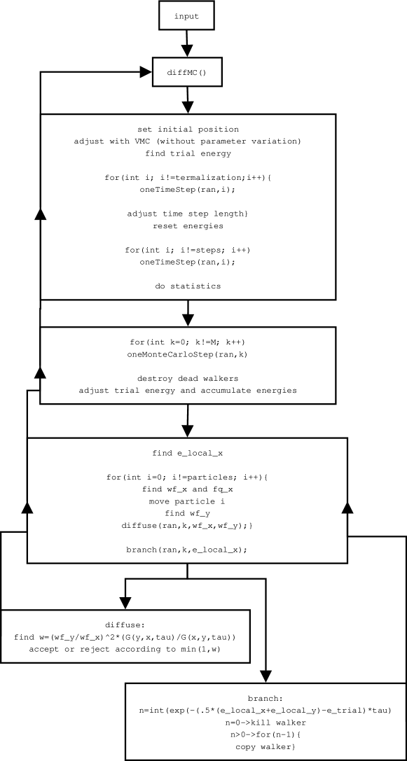
Figure 2: Float diagram of DMC

Fig. 2 shows the float diagram of the DMC program. The algorithm is divided into functions so that, e.g., the function diffMC() contains a loop calling the function oneTimeStep(), which in turn loops over oneMonteCarloStep() and so on. Each such function is represented by a box in the float diagrams.

Looking at the float diagram, fig. 2, it is easy to realize that most of the time of computation is spent in the bottom boxes of the diagram. When implementing the DMC in Python the bottom boxes should be kept in C++ while only diffMC() (which is in broad lines the hole DMC algorithm) will be in Python code.

IV.1.1 Checkpointing

And aspect which is frequently forgotten when writing a scientific program is the aspect of checkpointing. A Monte Carlo simulation may easily take several days, or even weeks and months. This would be unfeasible without some way to stop and start the simulation in case of computer crashes, power losses or overeager computer managers. In checkpointing we store all information needed to resume the computation at given steps of the simulation. The challenge is to identify the steps at which the checkpointing should be made. The checkpoints should be made frequently enough to save time compared to starting all over, but not so frequently that the simulation is significantly slowed down.

In variational Monte Carlo it suffices to write a new initialization file where the number of steps is reduced to what is remaining of the original number of steps and a random seed so that we continue the random stream we have started. The latter is important if we want to get reproducible results. As the amount of data stored in a checkpoint is so small, we can do it after every step without reducing speed. However, making a checkpoint during the movement of the particles would be quite cumbersome and the amount of data needed to store the checkpoint would increase dramatically.

Again, diffusion Monte Carlo is more challenging. As generating a starting state in effect takes a variational Monte Carlo run, we have to store all the walkers at every checkpoint. This involves storing all particle positions, the last calculated local energy and quantum force (which is a vector) and so on, for every walker. In the C++ implementation this is realized by the functions getBuffer and setBuffer in the Walker objects. In a call to getBuffer the walker puts all it’s information into a character array. In a checkpoint these arrays are concatenated and dumped to file. When restarting the program, the arrays are read from the file and sent to the walkers through setBuffer. The checkpoints are, as for variational Monte Carlo, made after every time step.

IV.1.2 Generating random numbers

When all is said and done the most important function in a Monte Carlo method is the random number generator. The Monte Carlo integration depends on a walker’s ability to reach all points in phase space from its starting point. If the random numbers determining the movement of the walker are in some way correlated, the walker will lose this ability. A good random number generator is therefore of great importance. Consider the simple one-dimensional definite integral

$$F=\int_{0}^{1}\,f(x)dx$$ (43)

To solve this equation numerically, we approximate $F$ in terms of $F_{N}$:

$$F=\lim_{N\to\infty}\,F_{N}$$ (44)

where

$$F_{N}=\frac{1}{N}\sum_{i=1}^{N}f(x_{i}).$$ (45)

When we solve eq. (43) using Monte Carlo integration, we draw the sample points $\{x_{i}\}$ randomly from a given probability density function. However, as a computer only has a finite sized set of numbers available, we have to use random numbers generated from a pseudo-random number generator (PRNG). For every PRNG there is a finite number of pseudo-random numbers, known as the cycle length of the PRNG. When this cycle length is reached eq. (44) will cease to converge. This may not seem like a serious problem as the cycle length can be made quite large by using better PRNGs. However, we have to take care to choose a good PRNG. To take an example, the PRNG ran0 (see numerical_recipes ) has a cycle length of about $2.1\times 10^{9}$. On a 3.40GHz Intel(R) Xeon(TM) CPU ran0 takes 40 seconds to run through one cycle. It is obvious that using this (widely used) PRNG will lead to problems when a Diffusion Monte Carlo simulation takes several days of CPU time.

The generation of random numbers is a science in itself and, though of great importance to Monte Carlo methods, we will not go through this aspect in detail. We can advise the interested reader to read the introduction of donald_knuth . In the simulations in this paper we have used a 64-bit linear congruential generator with prime addend SPRNG ; testingPRNG which has a period of $2^{64}$. Linear congruential generators may have correlations between numbers that are separated by a power of 2. We should therefore take care to avoid using this generator in batches of powers of 2. In our case, this happens in all 3D simulations with variational Monte Carlo. In algorithm 1 we make 3 calls to the random generator to move one particle, then one call to determine whether the move should be rejected or accepted. This is repeated for every particle. In our case, this can be avoided by letting the acceptance/rejection procedure use another random stream than the movement and making sure these streams are uncorrelated with each other.

IV.2 Parallelizing the C++ implementation

To parallelize Variational Monte Carlo (VMC) is embarrassingly easy. As long as you ensure that all the calculations use different sets of random numbers (and thereby ensuring that the calculations are uncorrelated) the algorithm is parallelized by running an independent calculation on each node. The communication between the nodes is restricted to spreading the input parameters before the calculations and collecting the output after calculation. The parallel efficiency is essentially 100%, and the calculation can theoretically use any number of nodes without efficiency loss.

The parallelization of Diffusion Monte Carlo (DMC) is more cumbersome. This is due to the branching part in algorithm 2 where walkers are killed or reproduced. If we had parallelized DMC in a straight forward way, i.e., by starting one DMC run per node with different sets of random numbers and collected the results at the end, the walkers would be unevenly distributed among the processes, leading to an inefficient DMC code. For a DMC code to function properly it needs an as large as possible number of walkers to get a good representation of the wave function. A lot of unconnected DMC simulations will basically yield a set of not-so-good wave functions. We therefore have to collect all the walkers, remove dead walkers and make copies of the more virile walkers according to the branching process and then redistribute the walkers at every time step.

The parallelization is realized by a division of the walker array. A master node stores an array of the full number of walkers and distribute these walkers evenly between the slave nodes where the walkers are stored in smaller walker blocks. The preparation to sending and receiving the walker blocks is identical to the checkpoint procedure mentioned above, sans the file writing and reading. In fact we use the MPI_Pack procedure to pack the walkers for checkpointing, even in the serial program. The only difference is that we send and receive the walkers instead of writing to and reading from file.

The main problem left is then to ensure that the sets of random numbers in fact are independent.

IV.2.1 Generating random numbers in parallel

Generating random numbers in parallel is not as straight-forward as one may think. A common first approach is to start the same random generator on every node, varying the seed with the rank of the node as a factor to get independent streams and hoping that these streams are uncorrelated. The main problem with this approach is that random generators often have long-term correlations which is of little importance in the serial case, but may appear as short-term correlations in a parallel case SPRNG ; testingPRNG . In the extreme case, we may chose seeds yielding random numbers separated with exactly one cycle. In this case we will end up with $N_{CPU}$ identical streams, yielding $N_{CPU}$ identical simulations and extremely good (but wrong) statistics in the results. Several approaches to get safe streams in parallel are suggested in SPRNG ; testingPRNG and implemented in the SPRNG library which we use in our simulations.

IV.3 Python implementation I

The C++ implementation uses about 90% of the time in the walker objects and most of this time in computing local energies ($N^{3}$ operations where $N$ is the number of particles) in functions located in Func. In the python implementation of diffusion Monte Carlo (pyDMC) the classes Walker and Func are therefore linked into a shared library readable from Python, through a thin wrapper module, together with the functions from the DMC class below the function oneTimeStep() in fig. 2.

The main obstacle in implementing pyDMC is the handling of the walkers. In a straight forward approach we put the walker objects in a native Python array. This is a very tempting approach; we can leave the entire problem of creating and killing walkers to Python. Another approach is to make a walker array class in C++. This way we can avoid explicit looping in the Python code, but we are again left to take care of varying array sizes in C++.

To understand the first approach, we must have a look at how to put the walkers into a native array. To get a C++ class visible from Python it has to be compiled and linked into a shared library. This step is taken care of by the use of SWIG swig . The walker array is then realized by the function warray, listing 1.

Listing 1: warray function

⬇

def warray(self,size,particles,dim):

"""function returning an array of (initialized) walkers"""

w = []

for i in range(size):

w += [Walker()]

w[i].pyInitialize(particles,dim)

return w

A great advantage with Python is that you can expand a class in run-time (or in fact build an entire class in run-time). Utilizing this advantage, we have inserted the function warray into the class Walker where it naturally belongs, as can be seen in the function funcToMethod, listing 2.

Listing 2: funcToMethod

⬇

def funcToMethod(func, clas, method_name=None):

"""function to insert a python func into a class

Taken from Python Cookbook, recipe 5.12"""

setattr(clas, method_name or func.__name__, func)

funcToMethod(warray,Walker) #insert function warray in class Walker

This approach is particularly handy if we want to expand the Func class with new physical systems, enabling us to write the new functors in pure Python code. However, as the functors are where most of the computation time takes place, this approach will severely hinder the effectiveness of the simulation.

In the native array approach most of the parallelization is realized with the functions spread_walkers and gather_walkers, listing 3.

Listing 3: Spread and gather

⬇

def spread_walkers(self):

"""Function converting walkers to numpy arrays, sending,

recieving and converting back"""

if self.master:

displace = self.loc_walkers[self.master_rank]

for i in range(1,self.numproc):

send_w = self.w[displace:displace+self.loc_walkers[i]]

send_buff = walkers2py(send_w)

self.pypar.send(send_buff,i)

displace += self.loc_walkers[i]

else:

recv_buff = self.pypar.receive(self.master_rank)

w_args = [self.loc_walkers[self.myrank], self.particles,\

self.dimensions]

self.w_block = py2walkers(recv_buff, *w_args)

def gather_walkers(self):

"""Look at spread_walkers in a mirror"""

if self.master:

displace = self.loc_walkers[self.master_rank]

for i in range(1,self.numproc):

recv_buff = self.pypar.receive(i)

w_args = [self.loc_walkers[i], self.particles,\

self.dimensions]

self.w[displace:displace+self.loc_walkers[i]] = py2walkers(\

recv_buff, *w_args)

displace += self.loc_walkers[i]

else:

send_buff = walkers2py(self.w_block)

self.pypar.send(send_buff,self.master_rank)

The functions walkers2py and py2walkers are functions for converting a walker to a NumPy array and back again, taking advantage of the functions getBuffer and setBuffer in the Walker class.

An example of a parallelized diffusion Monte Carlo program is realized in less than 100 lines:

⬇

>>> import pypar,math

>>> from DMC import DMC

>>>

>>> d = DMC(pypar)

>>> # 1 particle and alpha=0.5 yields a harmonic oscillator with

>>> # energy == 3/2:

>>> d.params[0] = 0.5

>>> d.reset_params()

>>> d.silent = True # to avoid too much noise

>>>

>>> def timestep(i_step):

… M = d.no_of_walkers

… d.spread_walkers()

… for walker in d.w_block:

… d.monte_carlo_step(walker)

… d.gather_walkers()

… d.update = False

… if d.master:

… #bring out your dead

… for i in range(M-1,-1,-1):

… if d.w[i].isDead():

… d.w[i:i+1] = [] #removing walker

… else:

… while d.w[i].tooAlive():

… baby_walker = d.copy_walker(d.w[i])

… baby_walker.calmWalker()

… d.w += [baby_walker]

… d.w[i].madeWalker()

… d.no_of_walkers = len(d.w)

… d.no_of_walkers = d.pypar.broadcast(d.no_of_walkers,

… d.master_rank)

… d.refresh_w_blocks()

… d.spread_walkers()

… d.num_args[-1] = d.update

… if d.master:

… nrg = 0.; pot_nrg = 0.; vort_nrg = 0

… d.time_step_counter += 1

… for walker in d.w:

… d.num_args[-1] = d.update

… nrg += walker.getLocalEnergy(*d.num_args)

… pot_nrg += walker.getLocalEnergy(d.pot_e)

… if hasattr(d,’vort_e’):

… vort_nrg += walker.getLocalEnergy(vort_e)

… nrg /= float(d.no_of_walkers*d.particles*d.scale)

… pot_nrg /= float(d.no_of_walkers*d.particles*d.scale)

… vort_nrg /= float(d.no_of_walkers*d.particles*d.scale)

… d.energy += nrg

… d.energy2 += nrg*nrg

… if d.time_step_counter >= d.termalization:

… #implement pos_hist to be called here

… d.observables[i_step,0] = nrg

… d.observables[i_step,1] = pot_nrg

… d.observables[i_step,2] = vort_nrg

… # adjust trial energy (and no. of walkers)

… nrg = -.5*math.log(float(d.no_of_walkers)/float(M))/d.tau

… d.e_trial += nrg

… d.e_trial = d.pypar.broadcast(d.e_trial,d.master_rank)

… d.no_of_walkers = d.pypar.broadcast(d.no_of_walkers,

… d.master_rank)

…

>>> #set initial walker positions:

>>> if d.metropolis_termalization: d.uni_dist()

…

>>> for i in range(d.metropolis_termalization):

… for walker in d.w_block:

… d.metropolis_step(walker)

…

>>>

>>> nrg = 0.

>>>

>>> for walker in d.w_block:

… nrg += walker.getLocalEnergy(*d.num_args)

…

>>> d.gather_walkers()

>>> d.e_trial = d.all_reduce(nrg)

>>> d.time_step_counter = 0

>>> for i in range(d.termalization):

… timestep(i)

…

>>> d.energy = 0; d.energy2 = 0

>>> for i in range(d.steps):

… timestep(i)

…

>>> if d.master:

… d.energy /= float(d.steps)

… d.energy2 /= float(d.steps)

… d.energy2 -= d.energy*d.energy

… print "energy = %g +/- %g"%(d.energy,

… math.sqrt(d.energy2/float(d.steps)))

… print "sigma = %g"%d.energy2

…

energy = 1.5 +/- 0

sigma = 0

>>> pypar.Finalize()

IV.4 Python implementation II

When thinking performance of arrays in Python the add-on package Numerical Python (NumPy) springs to mind as an obvious choice. The fact that the module pypar (which we are going to use in the parallelization) supports sending NumPy arrays directly, is of course helping in that choice. However, even though NumPy supports a lot of types, (such as integers, floats, chars etc.) there is no support for walkers as a type. It is possible to use generic python objects in NumPy arrays, but this will mainly make NumPy array comparable to native arrays.

The approach with native python arrays is quite straight-forward and easy to implement. It is, however, quite inefficient as well. There are two main reasons for this. First, looping is known to be an inefficient construct in Python. With a native Python array, the loops over walkers have to be done in Python. Second, native python arrays are slower than, e.g., NumPy arrays, because native arrays are written for a much more general use than just numerics. The question is how we can use the most of the C++ walker code as-is while avoiding explicit for-loops in Python.

One solution is to implement an array class (lets call it WalkerArray) in Python which is wrapper class to a C++ class containing a C++ array of walkers and functionality to create and kill walkers. Even though this is a good approach in a serial implementation, we still have to convert these arrays to NumPy arrays to be able to send the walkers in MPI.

In our Python implementation, we keep the WalkerArray, but store all the walker data in a NumPy array. To do this we have modified the C++ Walker class so that it only uses pointers to an array for all arrays and variables that should be stored. This array is then provided by NumPy. Even though this approach taints the C++ implementation of the Walker class, we get the advantage that the Python DMC class only has to care about NumPy arrays, providing us with powerful tools for vectorizing the Python code.

IV.4.1 WalkerArray

To implement the class WalkerArray we need to have some knowledge of the C++ Walker class. The Walker class contains some arrays storing all particle positions and all previous particle positions and variables to know if the walker should be removed or duplicated. In addition it stores the last computed local energy, quantum force and wave function to minimize the number of times we compute these quantities. In the C++ code this information is allocated and stored in each walker, making the creation of a walker rather costly. When we send walkers in MPI the information is collected from each walker and concatenated into one array before communication and inserted into the walkers after communication. Now, we want turn it the other way, i.e., we want to allocate and store all information from all walkers in one array (preferably a NumPy array) and let the walkers operate on pointers to this array. This way the time to initialize a walker is reduced dramatically and all information on walkers are readily available from Python. This change of view for the Walker class is realized by changing all variables that define the walker to references to the corresponding pointers to the NumPy array.

V Python vs. C++

Now we know how to implement a Python version of a Monte Carlo solver. We then need to know if MontePython is efficient enough. We can assume that the Python implementation will never be faster that the corresponding C++ code, as Python will always have some degree of overhead just to access the C++ code. The question is how big this overhead may be.

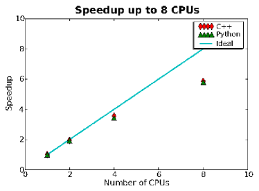
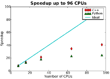
Figure 3: Speedup of a simulation as a function of the number of CPUs used. In the left figure the serial run took about 30 minutes and was run with an initial 480 walkers moved in 3500 time steps. In the right figure the serial run took about 4 hours 30 minutes and was run with an initial 4800 walkers moved in 1750 time steps.

In figure 3 we have plotted the speedup of a Monte Carlo simulation as a function of the number of CPUs. To the left we have done a relatively light simulation with 20 particles in 3 dimensions using 480 walkers. The walkers are spread out evenly and communicated from the master node to the slave nodes and back again 3500 times so that all walkers are sent 7000 times. The size of one walker is in this case $1.2$kB which means that for, e.g., 4 CPUs the size of each message is about 144kB. We can see that for this message size the overhead of using Python is almost none.

To the right in figure 3 we have increased the number of walkers to 4800. However, we are also using a much higher number of CPUs. The message size for, e.g., 64 CPUs is only 9kB. As we explicitly loop over the number of CPUs when we send walkers to and from the master, the overhead increases dramatically when compared to the time to send one message. The send and receive methods should therefore be vectorized with scatter and gather routines. Unfortunately we do not have uniform message sizes, making generic scatter and gather routines unusable. We will therefore have to write these routines ourselves.

Python has similar speedup to C++, but the curve flattens out much faster as we increase the number of CPUs. As Monte Carlo simulations are known to have perfect speedup, we cannot be satisfied with the parallel algorithms of either the C++ version or the Python version.

VI Optimizing MontePython

One of the points in using Python in scientific programming is that you can implement new and improved algorithms efficiently. We have seen that distribution of the random walkers over the compute nodes leads to a bottleneck due to communication when the number of CPUs grows large. This bottleneck is evident both for the C++ implementation and the Python implementation. In this section we will improve the algorithm for load balancing of the walker in two ways. First, we will improve on the way the walkers are killed and reproduced. Second, we will improve on the load balancing itself by optimizing for heterogeneous clusters of CPUs.

VI.1 Distributing Walkers in Parallel

The C++ Diffusion Monte Carlo application was originally written in serial and then ported to parallel using MPI. In the serial version we used an algorithm where, in order to kill a walker, we moved the last walker in the sequence onto the walker that was to be killed and decreased the number of walkers with one. To reproduce a walker, we copied the walker to the end of the sequence. This algorithm is optimal and widely used in serial Diffusion Monte Carlo. When we parallelized the code, we kept this serial algorithm by gathering all the walkers to the master node, let the master node do the killing and reproducing in serial, and then spread the walkers evenly among the slave nodes again. This way the load was always balanced, and the master had full control of the walkers at all times. The main problem is that, apart from memory issues as the master needs to store a lot of walkers, the serial work load for the master increases fast when we increase the number of CPUs in the calculation. This problem is very clear in figure 3, where the speedup is quite poor already for 32 CPUs, both for the C++ version and the Python version.

Again, the algorithm is best explained through the source code. First we let the slave nodes individually move their walkers and kill and reproduce their local walkers, then the function DMC.load_balancing(),balances the load:

⬇

1 def load_balancing(self):

"""Function balancing load between nodes"""

3 self.t1 = time.time()

w_numbers = self.pypar.gather(Numeric.array([len(self.w_block)]),

5 self.master_rank)

tmp_w_numbers = copy.deepcopy(w_numbers)

7 w_numbers = self.pypar.broadcast(tmp_w_numbers,

self.master_rank)

9

self.no_of_walkers = Numeric.sum(w_numbers)

11

self.__find_opt_w_p_node()

13

self.first_balance = False

15 balanced = Numeric.array(self.loc_walkers)

17 difference = w_numbers-balanced

19 diff_sort = Numeric.argsort(difference)

prev_i_min = diff_sort[0]

21

while sum(abs(difference))!=0:

23 diff_sort = Numeric.argsort(difference)

i_max = diff_sort[-1]

25 i_min = diff_sort[0]

27 if i_min == prev_i_min:

i_min = diff_sort[1]

29

if self.myrank==i_max:

31 self.pypar.send(self.w_block[balanced[i_max]:],i_min)

args = [balanced[i_max],

33 self.particles,

self.dimensions,

35 self.w_block[0:balanced[i_max]]]

self.w_block = WalkerArray.WalkerArray(*args)

37 elif self.myrank==i_min:

recv_buff = self.pypar.receive(i_max)

39 args = [len(self.w_block)+difference[i_max],

self.particles,

41 self.dimensions,

Numeric.concatenate((self.w_block[:],recv_buff))]

43 self.w_block = WalkerArray.WalkerArray(*args)

difference[i_min]+=difference[i_max]

45 difference[i_max]=0

prev_i_min = i_min

This function deserves some explanation. From line 5 to ‣ VI.1 we update the current walker distribution and total number of walkers. In line ‣ VI.1 we determine the optimal distribution of walkers. to be explained in subsection VI.2. At this point we know the actual distribution of walkers and the optimal distribution of walkers. The idea is then to find the length of the difference between the optimal and actual distribution and move walkers among nodes until the length, or the sum of the absolute value of the differences is is zero, see line ‣ VI.1. This is realized in lines ‣ VI.1-45 by moving the excess walkers from the node with maximum difference to the walker with minimum difference recursively. A problem with this procedure is that the the same node can have a minimum difference in subsequent cycles of the while-loop. This leads to unnecessary waiting in the program. The remedy is seen in line 27 where we take the second minimum node if the minimum node is the same node as in the previous cycle. Of course this problem may just be transferred to the second minimum node, but this is much less likely to happen.

It should be noted that this optimization does not preserve the result from the non-optimized code, in the sense that we will not get an identical output in the end. This is due to the fact that the random sequences are distributed per node and not per walker, meaning that each walker will get a different series of random numbers depending on which node it is sent to. The output will, however, be within the error range of the non-optimized code.

VI.2 Heterogeneous clusters

Most new high performance clusters are more or less homogeneous, in the sense that the computation nodes have identical specifications with respect to CPU, RAM, network and storage. However, as a cluster usually expands in time, due to more funds and need for more resources, it is very likely that it will become a heterogeneous cluster. Also, with the trend of multiple cores and CPUs per computation nodes, combined with the fact that there is more than one user per cluster, different nodes will have different (and possibly too high) load and therefore different computational speed. This means that even if a cluster is homogeneous on paper, it will act like a heterogeneous cluster in practice. If we want to gain the optimal performance from a cluster, we need to take into account this heterogeneity.

In the function __find_opt_w_p_node() we use the time from the DMC class is initialized to the function is called to determine how the optimal distribution of walkers at every time step. The function itself can be seen in listing 4.

Listing 4: Finding optimal walkers per node

⬇

1 def __find_opt_w_p_node(self):

"""Help function for load_balancing()

3 Finds and returns the optimal number of walkers

per node for a possibly non-uniform set of nodes

5 """

self.t1 = time.time()

7 timings = self.pypar.gather(Numeric.array([abs(self.t1-self.t0)]),

self.master_rank)

9 tmp_timings = copy.deepcopy(timings)

timings = self.pypar.broadcast(tmp_timings,

11 self.master_rank)

13 C = self.no_of_walkers/sum(1./timings)

15 tmp_loc_walkers = C/timings

17 self.loc_walkers = self.NumericFloat2IntList(tmp_loc_walkers)

remainders = tmp_loc_walkers-self.loc_walkers

19

while sum(self.loc_walkers) < self.no_of_walkers:

21 maxarg = Numeric.argmax(remainders)

self.loc_walkers[maxarg] += 1

23 remainders[maxarg] = 0

25 if self.master and self.first_balance:

print timings

27 print self.loc_walkers

29 return self.loc_walkers

To understand this function we just need some simple linear algebra. Say that we have set of walkers ${[x_{1},x_{2},\ldots x_{N}]}$ spread in an optimal way over $N$ nodes. On node $i$ the time to move one walker is given by $a_{i}$ yielding a set ${[a_{1},a_{2},\ldots a_{N}]}$. By optimal distribution we mean a distribution of walkers were each node finishes the work assigned to it between synchronizations at the same time $C$, i.e. ${a_{i}x_{i}=C}$. In addition we know the total number of walkers, $T$. We know that

$$\sum x_{i}=\sum\frac{C}{a_{i}},$$ (46)

so that the problem reduces to finding $C$. However, as $T=\sum x_{i}$, we have

$$C=\frac{T}{\sum 1/a_{i}}.$$ (47)

The zealous reader will notice that eq. (47) corresponds to line 13 of __find_opt_w_p_node(). The rest of the function is merely taking care of the fact that $x_{i}$ are integers while $a_{i}$ and $C$ are real numbers.

VI.3 Optimized results

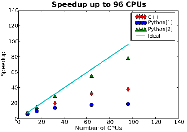
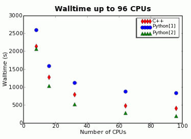
Figure 4: The figures show the speedup (left figure) and walltime (right figure) for the simulation as a function of the number of CPUs used. The serial run took about 270 minutes and was run with an initial 4800 walkers moved in 1750 time steps.

In figure 4 we show the speedup and walltime of the improved walker distribution compared to the non-optimized C++ and Python version from figure 3. We see that both the speedup and the walltime is much more reasonable for the optimized version of MontePython. In fact, the new version is more than twice as fast as the C++ version for 96 CPUs.

These optimizations would of course be possible to do in the C++ application as well, albeit in more than 75 lines. However, the simple syntax in Python and the use of Numeric arrays to store walkers allow us to concentrate our effort directly on the optimization of the algorithm instead of dealing with, e.g., how to send, receive and concatenate a slice of walkers.

VII Visualizing with Python

We mentioned in the introduction that integration of simulation and visualization is an important feature of Matlab, Maple and others. This feature is maybe even more powerful in Python. In figures 5, 6 and 6 we have used pyVTK and Mayavi mayavi to plot the particle density, which is an output of diffusion Monte Carlo. pyVTK pyvtk is a python interface to the Visualization ToolKit (VTK), while Mayavi, which is built on pyVTK, is a scriptable graphic interface for 3D visualization.

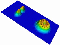
Figure 5: The figures show where particles are detected. We see the expectation values in two spatial dimensions, the $yz$-plane to the left and the $xy$-plane to the right. The topmost figure corresponds to the ground state, while the bottom figure corresponds to a state with one vortex in the center of the trap.

A signature of a Bose-Einstein condensate is that it is irrotational. If we try to rotate the condensate, it will compensate by setting up quantum vortices along the rotational axis. Vortices is therefore crucial to the study of Bose-Einstein condensates. We need only small modifications to the Hamiltonian (eq. (3)) and trial wave function (eq. (4)) to consider a single vortex along the $z$-axis in our system nilsen2005 .

Figures 5 and 6 shows the change in the ground state when inserting the vortex. The repulsive nature of the vortex pushes the particles away from the $z$-axis, decreasing the maximum density when compared to the ground state.

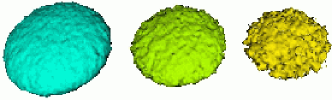
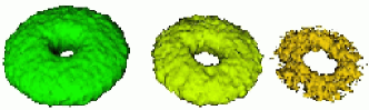
Figure 6: The figures show where particles are detected. We see the expectation values for finding, from left to right, 1, 2, 3 and 4 particles. The topmost figure corresponds to the ground state, while the bottom figure corresponds to a state with one vortex in the center of the trap.

VIII Conclusion

We have implemented a Monte Carlo solver using three different approaches, from pure C++, through a straight forward Python implementation, to an efficient, vectorized Python implementation. Furthermore we have compared the C++ and the vectorized Python implementations and shown that the overhead of using Python is non-existent for sufficiently large problems. In fact, with only 75 lines of code we were able to introduce an improved parallel algorithm for walker distribution, to gain a super-linear speedup when compared to C++. In addition, we have shown that Python can be used directly as a visualization tool for rendering three dimensionally scientific visualizations. We can therefore safely say that Python serves as a powerful tool in scientific programming.

References

- (1) Guido van Rossum et al. The Python programming language, 1991–.
- (2) Pearu Peterson Eric Jones, Travis Oliphant et al. SciPy: Open source scientific tools for Python, 2001–.
- (3) David Beazley et al. SWIG: Simplified wrapper and interface generator, 1995–.
- (4) J.L. DuBois and H.R. Glyde. Natural orbitals and bec in traps, a diffusion monte carlo analysis. Phys. Rev. A, 68, 2003.
- (5) A. Harju. Variational monte carlo for interacting electrons in quantum dots. Journal of Low Temperature Physics, 140:181–210, 2005.
- (6) J.R. Anderson, M.R. Ensher, M.R. Matthews, C.E. Wieman, and E.A. Cornel. Observation of bose-einstein condensation in a dilute atomic vapor. Science, 269:198, 1995.
- (7) J.K. Nilsen, J. Mur-Petit, M. Guilleumas, M. Hjorth-Jensen, and A. Polls. Vortices in atomic bose-einstein condensates in the large gas parameter region. Phys. Rev. A, 71, 2005.
- (8) J.L. DuBois and H.R. Glyde. Bose-einstein condensation in trapped bosons: A variational monte carlo analysis. Phys. Rev. A, 63, 2001.
- (9) N. Metropolis, A. W. Rosenbluth, M. N. Rosenbluth, A. M. Teller, and E. Teller. Equations of state calculations by fast computing machines. J. Chem. Phys., 21:1087, 1953.
- (10) B.L. Hammond, W.A. Lester Jr, and P.J. Reynolds. Monte Carlo Methods in Ab Initio Quantum Chemistry. World Scientific, 1994.
- (11) R. Guardiola. Monte carlo methods in quantum many-body theories. In J. Navarro and A. Polls, editors, Microscopic Quantum Many-Body Theories and Their Applications, Lecture Notes in Physics, pages 269–336. Springer Verlag, 1997.
- (12) P. J. Reynolds, D.M. Ceperley, B. J. Alder, and W. A. Lester Jr. J. Chem. Phys., 77:5593, 1982.
- (13) A. Sarsa, J. Boronat, and J. Casulleras. Quadratic diffusion monte carlo and pure estimators for atoms. Phys. Rev. A, 2001.
- (14) W.H. Press, S.A. Teukolsky, W.T. Vetterlin, and B.P. Flannery. Numerical Recipes in C, Second Edition. Cambridge University Press, 2002.
- (15) D.E. Knuth. The Art of Computer Programming, Second Edition. Addison-Wesley Publishing Company, 1981.
- (16) M. Mascagni and A. Srinivasan. Sprng: A scalable library for pseudorandom number generation. ACM Transactions on Mathematical Software, 26:436–461, 2000.
- (17) A. Srinivasan, M. Mascagni, and D. Ceperley. Testing parallel random number generators. Parallel Computing, 29:69–94, 2003.
- (18) P. Ramachandran. Mayavi: A free tool for cfd data visualization. In 4th Annual CFD Symposium. Aeronautical Society of India, 2001.
- (19) Pearu Peterson. PyVTK: Tools for manipulating vtk files in python, 2001–.