Single DNA conformations and biological function

Abstract

Abstract. From a nanoscience perspective, cellular processes and their reduced in vitro imitations provide extraordinary examples for highly robust few or single molecule reaction pathways. A prime example are biochemical reactions involving DNA molecules, and the coupling of these reactions to the physical conformations of DNA. In this review, we summarise recent results on the following phenomena: We investigate the biophysical properties of DNA-looping and the equilibrium configurations of DNA-knots, whose relevance to biological processes are increasingly appreciated. We discuss how random DNA-looping may be related to the efficiency of the target search process of proteins for their specific binding site on the DNA molecule. And we dwell on the spontaneous formation of intermittent DNA nanobubbles and their importance for biological processes, such as transcription initiation. The physical properties of DNA may indeed turn out to be particularly suitable for the use of DNA in nanosensing applications.
Key words: DNA, single molecules, DNA looping, DNA denaturation, knots, gene regulation

I Introduction

Deoxyribonucleic acid (DNA) is the molecule of life as we know it. It contains all information of an entire organism. This information is copied during cell division with an extremely high fidelity by the replication mechanism. Despite the rather high chemical and physical stability of DNA, due to constant action of enzymes and other binding proteins (mismatches, rupture) as well as potential environmentally induced damage (radiation, chemicals), this low error rate, i.e., the suppression of the liability to mutations, is only possible with the constant action of repair mechanisms alberts ; snustad ; kornberg ; kornberg1 . Although DNA’s structural and mechanical properties are rather well established for isolated DNA molecules (starting with Rosalind Franklin’s X-ray diffraction images franklin ), the characterisation of DNA in its cellular environment, and even in vitro during interaction with binding proteins, is subject of ongoing investigations.

Recent advances in experimental techniques such as fluorescence methods, atomic force microscopy, or optical tweezers have leveraged the potential to both probe and manipulate the equilibrium and out of equilibrium behaviour of single DNA molecules, making it possible to explore DNA’s physical and mechanical properties as well as its interaction with other biopolymers, such as the DNA-protein interplay during gene regulation or repair processes. An important ingredient is the coupling to thermal activation due to the highly Brownian environment. Although mostly performed in vitro, these experiments provide access to increasingly refined information on the nature of DNA and its environment-controlled behaviour.

In addition to chromosomal packaging inside the nucleus of eukaryotic cells and the concentration of DNA in the membraneless nucleoid region of prokaryotes, the global structure of the DNA molecule can be affected by topological entanglements. Thus, by error or design a DNA molecule can attain a knotted or concatenated state, reducing or inhibiting biologically relevant functions, for instance, replication or transcription. Such entangled states can be actively reduced by enzymes of the topoisomerase family. Their precise action, in particular, how they determine the presence of an entangled state, is not fully known. Current studies therefore aim at shedding light on possible mechanisms, in particular, in view of the importance of topoisomerase action (or better, its inhibition) in tumour proliferation. Other applications may be directed towards the treatment of viral deceases by modifying the packaging of viral DNA to create knots in the virus capsid and prevent ejection of the DNA into a host, and thereby infection. DNA knots are also being recognised as a potential complication in the use of nanochannels for DNA separation and sequencing. In such confined geometries DNA knots are created with appreciable probability, affecting the reliability of these techniques. Similarly to DNA knots, DNA looping is intimately connected to the function of DNA. Current results on DNA looping and DNA knot behaviour are summarised in the first parts of this review.

The Watson-Crick double-helix represents the thermodynamically stable state of DNA at moderate salt concentrations and below the melting temperature. This stability is effected by Watson-Crick hydrogen bonding and the stronger base stacking of neighbouring base-pairs (bps). However, even at room temperature DNA locally opens up intermittent flexible single-stranded domains, so-called DNA-bubbles. Their size typically ranges from a few broken bps, increasing to some 200 broken bps closer to the melting temperature. The thermal melting of DNA has traditionally been used to obtain the sequence-dependent stability parameters of DNA. More recently, the role of intermittent bubble domains has been investigated with respect to the liability of DNA-denaturation induced by proteins that selectively bind to single-stranded DNA. It has been speculated that due to the liability to denaturation of the TATA motif bubble formation may add in transcription initiation. The dynamics of single bubbles can be monitored by fluorescence methods, opening a window to both study the breathing of DNA experimentally, but also to obtain high precision DNA stability data. Finally, bubble dynamics has been suggested as a useful tool in optical nanosensing. DNA breathing is the topic of the second part of this work.

Essentially all the biological functions of DNA rely on site-specific DNA-binding proteins locating their targets (cognate sites) on the DNA molecule, and therefore require searching through megabases of non-target DNA in a highly efficient manner. For instance, gene regulation is performed by specific regulatory proteins. On binding to a promoter area on the DNA, they recruit or inhibit binding of RNA polymerase and subsequent transcription of the associated gene. The search for the cognate site is in fact facilitated by the DNA molecule: in addition to three-dimensional search it enables the proteins to also move one-dimensionally along the DNA while being non-specifically bound. Moreover, at points where the DNA loops back on itself, this polymeric conformation provides shortcuts for the proteins in the chemical coordinate along the DNA, approximately giving rise to search-efficient Lévy flights. Target search is currently a very active field of research, and single molecule methods have been shown to provide essential new information. Moreover, the architecture of more complex promoters relying on the simultaneous presence of several regulatory proteins is being investigated to create in silico circuits for highly sensitive chemical probes in small volumes. Such nanosensing applications are expected to be of great importance in microarrays or other nano- and microapplications. The third part of this review deals with diffusional aspects of gene regulation.

At the same time DNA’s role in classical polymer physics is increasingly appreciated. With the possibility to reproduce DNA with extremely low error rate by the PCR, monodisperse samples can be prepared. While shorter single-stranded DNA can be used as a model for flexible polymers, the double strand exhibits a semiflexible behaviour with a persistence length, that can be easily probed experimentally. Moreover, DNA is orders of magnitude longer than conventional polymers. Combined with the potential of single molecule probing, DNA is advancing as a model polymer.

After an introduction to the properties of DNA we address these functional properties of DNA from the perspective of biological relevance, physical behaviour and nanotechnological potential. Most emphasis will be put on the single molecular aspects of DNA. We note that this is not intended to be an exhaustive review on the physical properties of DNA. Rather, we present some important features and their consequences from a personal perspective.

II Physical properties and biological function of DNA

Biomolecules, that occur naturally in biological systems, can be grouped into unspecific oligo- and macromolecules and biopolymers in the stricter sense alberts . Unspecific biomolecules are produced by biological organisms in a large range of molecular weight and structure, such as polysaccharides (cellulose, chitin, starch, etc.), higher fatty acids, actin filaments or microtubules. Also the natural ‘india-rubber’ from the Hevea Brasiliensis tree, historically important for both industrial purposes and the development of polymer physics treloar belongs to this group.

Figure 1: Central dogma of molecular biology after F. Crick: Potentially, information flow is completely symmetric between the three levels of cellular biopolymers (DNA, RNA, proteins). However, the recognised pathways are only those represented here, where solid lines represent probable transfers, and dotted lines for (in principle) possible transfers crick .

Biopolymers in the stricter sense we are going to assume here comprise the polynucleotides DNA and RNA consisting of the four-letter nucleotide alphabet with A-T and G-C (A-U and G-C for RNA) bps, and the polypeptidic proteins consisting of 20 different amino acids, each coded for by 3 bases (codons) in the RNA alberts ; snustad ; kornberg ; kornberg1 . We will come back to proteins later when reviewing binding protein-DNA interactions. Biopolymers are copied and/or created according to the information flow sketched in figure 1, the so-called central dogma of molecular biology, a term originally coined by Frances Crick crick1 . Accordingly, starting from the genetic code stored in the DNA (in some cases in RNA) DNA is copied by DNA polymerase (replication), and the proteins as the actually task-performing biopolymers are created via messenger RNA (created by DNA transcription through RNA polymerase) and further by translation in ribosomes to proteins.

DNA is made up of the four bases alberts ; snustad ; kornberg ; kornberg1 ; bloomfield ; rnaworld : A(denine), G(uanine), C(ytosine), and T(hymine) that form the DNA ladder structure shown in figure 2.

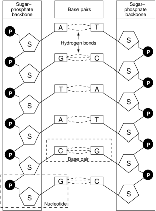
Figure 2: Ladder structure of the DNA formed by its four building-blocks A, G, C, and T, giving rise to the typical double-helical structure of DNA. A-T bps establish 2 H-bonds, G-C bps 3 H-bonds.

These building-blocks A, G, C, T bp according to the key-lock principle as A-T and G-C, where the AT bond is weaker than the GC bond in terms of stability. Apart from the Watson-Crick base-pairing energy, the stability of dsDNA is effected by the stacking interactions, the specific matching of subsequent bps along the double-strand, i.e., bp-bp interactions. In standard literature, the stacking interactions are listed for pairs of bps (e.g., for AT-GC, AT-AT, AT-TA, etc.), see below.

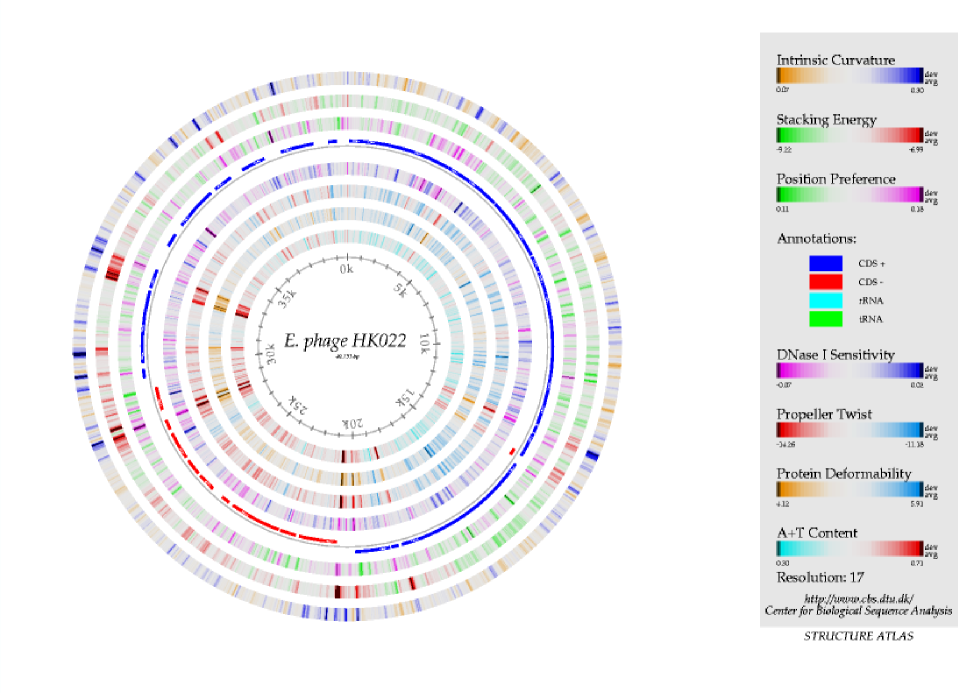
Figure 3: Structure atlas of the E.coli genome. Figure courtesy David Ussery, Technical University of Denmark. The structure atlas is available under the URL www.cbs.dtu.dk/services/GenomeAtlas/.

Based on this AGCT alphabet, the primary structure of DNA can be specified. DNA’s six local structural elements twist, tilt, roll, shift, slide, and rise are effected by the stacking interactions between vicinal bps. In figure 3, we show a map with the structure elements of the entire E.coli genome, demonstrating the degree of structural information currently available. These structural elements define the local geometrical structure of DNA within a typical correlation (persistence) length of about 150 bps corresponding to 50 nm (the bp-bp distance measures 3.4 Å, reflecting the rather complex chemical structure of a nucleotide in comparison to the monomer size of man-made polymers such as polyethylene) frank ; frank1 ; marko ; marko1 . On a larger scale, much longer than the persistence length, DNA becomes flexible. On this level, tertiary structural elements come into play. One example is DNA looping, that is the formation of polymeric lasso loops induced by chemical bonds between binding proteins attached to the DNA at specific bps which are remote along the DNA backbone alberts ; snustad ; ptashne1 ; revet ; bell ; bell1 ; hame_looping . An extreme limit of tertiary structure is the packaging of DNA onto histones and further wrapping into the chromosomes of eukaryotic cells schiessel ; kreth ; alberts . At the same time, dsDNA may locally open into floppy ssDNA bubbles, with a persistence length of a few bases. These fluctuation-induced bubbles increase their statistical weight at higher temperatures, until the dsDNA fully denatures (melts). We will come back to DNA denaturation bubbles below. Depending on the external conditions, DNA occurs in several configurations. Under physiological conditions, one is concerned with B-DNA, but there are other states such as A, B’, Z, ps, triplex DNA, quadruplex DNA, cruciform, and H, reviewed, for instance, in frank ; frank1 . DNA occurs naturally in a large range of length scales. In viruses, DNA is of the order of a few $\mu$m long. In bacteria, it already reaches lengths of several mm, and in mammalian cells it can reach the order of a few m, roughly 2 m in a human cell and 35 m in a cell of the South American lungfish, albeit split up into the individual chromosomes kornberg . DNA in bacteria in vivo, or extracted from bacteria and higher cells for our purposes can therefore be viewed a fully flexible polymer with a persistence length of roughly 50 nm, being governed by generic effects independent of the detailed sequence. On short scales DNA becomes semiflexible and governed by the worm-like chain model (Kratky-Porod model) grosberg ; on even shorter scales, local structural elements become important (in particular, for recognition by binding proteins alberts ), and eventually molecular resolution is reached.

Stacking interactions govern the local structure of dsDNA. Globally, an additional constraint arises due to the circular nature of the DNA, since it has to satisfy the conservation law calu ; white1 ; fuller

$${\rm Lk}={\rm Tw}+{\rm Wr},$$ (1)

where Lk stands for the linking number, Tw for the twist, and Wr for the writhe of the double helix. The linking number $Lk$ is an integer and formally given by one-half the number of signed crossings of one DNA strand with the other in any regular projection of the molecule. $Lk$ is a topological property, and no deformation of a closed DNA, without breaking and rejoining the DNA strands, will alter it. $Tw$ is equal to the number of times that the two strands of DNA wind about the central axis of the molecule, and $Wr$ is a number whose absolute value equals approximately the number of times that the DNA axis winds about itself. Whereas Tw is a property of the double-helical structure of DNA, Wr is a property of the DNA axis alone. Tw and Wr do not need to be integers and are not conserved, but coupled through Lk by equation (1). A nicked circular DNA, i.e., when the twist can fully relax, carries ${\rm Lk}_{0}=N/h$ links, where $N$ is the number of bp and $h$ ($h\simeq 10.5$ in B-DNA) the number of bps per turn.

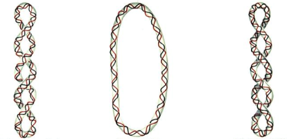
Figure 4: Right-handed (negative), normal, and left-handed (positive) superhelix. The DNA of virtually all terrestrial organisms is negatively supercoiled.

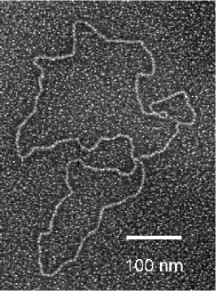
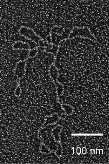
Figure 5: Electron micrographs of nicked (left) and supercoiled (right) 6996-bp plasmid DNAs. The supercoiled example is from a population of DNA molecules with an average superhelix density, $\bar{\sigma}$= -0.027, close to the value expected in vivo.

The degree of supercoiling of DNA can be expressed in terms of the linking number difference, $\Delta Lk=Lk-Lk_{0}$. The DNA of virtually all terrestrial organisms is underwound or negatively supercoiled, i.e., $\Delta Lk<0$ (figures 4 and 5). Often, the superhelical density $\sigma=\Delta Lk/Lk_{0}$ is used; most supercoiled DNA molecules isolated from either prokaryotes or eukaryotes have $\sigma$ values between $-0.05$ and $-0.07$ bauer . Negative supercoiling is regulated in prokaryotes by DNA gyrase; eukaryotes lack gyrase but maintain negative supercoiling through winding of DNA around nucleosomes and interactions with DNA-unwinding proteins. There are two forms of intracellular supercoiling, the plectonemic form, characteristic of plasmid DNA and accessible, nucleosome-free regions of chromatin, and the toroidal or solenoidal form, where supercoiling is attained by DNA wrapped around histone octamers or prokaryotic non-histone DNA-binding proteins (figure 6). The former is the active form of supercoiled DNA and is freely accessible to proteins involved in transcription, replication, recombination and DNA repair. The latter is the stored form of supercoiled DNA and is largely responsible for the extraordinary degree of compaction required to condense typical genomes into the cell’s nucleus. Negative supercoiling facilitates the local unwinding of DNA by providing a ubiquitous source of free energy that augments the unwinding free energy accompanying the interactions of many proteins with their cognate DNA sequences. The local unwinding of DNA, in turn, is an integral part of many biological processes such as gene regulation and DNA replication (see section VI). Therefore, understanding the interplay of supercoiling and local helical structure is essential to the understanding of biological mechanisms marko1 ; benham ; goetze ; levene ; levene1 .

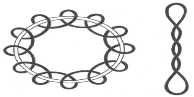
Figure 6: Toroidal (left) and plectonemic (right) forms of supercoiled DNA.

Ribonucleic acid (RNA) consists of the same building blocks as DNA, with the exception that T(hymine) is replaced by U(racile) rnaworld . RNA typically occurs in single-stranded form. Therefore, its secondary structure is richer, being characterised by sequences of hairpins: Smaller regions in which chemically remote sequences of bases match, pair and form hairpins which are stiff and energy-dominated, similar to dsDNA. The remaining regions form entropy-dominated floppy loops, analogous to the ssDNA bubbles. Additional tertiary structure in RNA comes about by the formation of so-called pseudoknots, chemical bonds established between bases sitting on chemically distant segments of the secondary structure. In RNA-modelling the incorporation of pseudoknots is a non-trivial problem, which currently receives considerable interest; see, for instance, references rnaworld ; orland ; orland1 ; baiesips .

III DNA-looping

The formation of DNA loops mediated by proteins bound at distant sites along a single molecule is an essential mechanistic aspect of many biological processes including gene regulation, DNA replication, and recombination (for reviews, see loop1 ; loop2 ). In E. coli, DNA looping represses gene expression at the ara, gal, lac, and deo operons loop3 ; loop4 ; loop5 ; loop6 and activates transcription from the glnALG operon loop7 . The size of DNA loops formed in these systems varies between approximately 100 and 600 bps. In eukaryotes, a variety of transcription factors bind to enhancers that are hundreds to several thousand bps away from their promoters and interact with RNA polymerases directly or through mediators in order to achieve combinatorial gene regulation loop8 . DNA looping is required to juxtapose two recombination sites in intramolecular site-specific recombination loop9 ; loop10 ; loop11 and is also employed by a number of restriction endonucleases such as SfiI and NgoMIV, which recognise and cut two copies of well-separated cognate sites simultaneously loop12 ; loop13 ; loop14 . Here we describe a recent statistical-mechanical theory of loop formation that connects global mechanical and geometric properties of both DNA and protein and demonstrates the importance of protein flexibility in loop-mediated protein-DNA interactions loop26 ; loop51 .

III.1 Biological significance of DNA looping

The biological importance of DNA loop formation is underscored by the abundance of architectural proteins in the cell such as HU, IHF, and HMG, which facilitate looping by bending the intervening DNA between protein-recognition sites loop15 . Moreover, DNA looping has been shown to be subject to regulation through the binding of effector molecules that alter protein conformation or protein-DNA interactions loop16 .

Two characteristics of DNA looping have been demonstrated by in vitro and in vivo experiments. One is cooperative binding of a protein to its two cognate sites, which can be demonstrated by footprinting methods loop17 . DNA looping can increase the occupancies of both binding sites; in particular, it can significantly enhance protein association to the lower-affinity site because of the tethering effect of DNA looping. This is a general mechanism by which many transcription factors recruit RNA polymerases in gene regulation. Another hallmark is the helical dependence of loop formation loop1 ; loop3 , which arises because of DNA’s limited torsional flexibility and the requirement for correct torsional alignment of the two protein-binding sites. Although many methods have been developed to directly observe DNA looping in vitro, such as scanning-probe loop7 and electron microscopy bloomfield , and single-molecule techniques loop19 , assays based on helical dependence have been the only way to identify DNA looping in vivo. In these experiments, the DNA length between two protein binding sites is varied and the yield of DNA loop formation is monitored, for example by the repression or activation of a reporter gene loop20 . Using this helical-twist assay, DNA looping in the ara operon was first discovered loop3 .

Our knowledge about the roles of DNA bending, twist, and their respective energetics in DNA looping has come largely from analyses of DNA cyclisation loop1 ; loop21 ; loop22 . Circularisation efficiencies of DNA fragments, which are quantitatively described by $J$-factors, oscillate with DNA length and therefore torsional phase loop23 ; loop24 . The $J$-factor is defined as the ratio of the partition function of a circularised polymer chain to that of an open chain. Since there is a dimension reduction due to circularisation constraints (two polymer ends have to meet), the ratio has a unit of concentration, or $1/L^{3}$ with $L$ representing length; see loop26 for details. In the present context, the $J$-factor is equal to the free DNA-end concentration whose bimolecular ligation efficiency equals that of the two ends of a cyclising DNA molecule loop25 . For short DNA fragments $J$-factors are limited by the significant bending and twisting energies required to form closed circles, whereas for long DNA, the chain entropy loss during circularisation exceeds the elastic-energy decrease and reduces the $J$-factor. Because of this competition between bending and twisting energetics and entropy, there is an optimal DNA length for cyclisation loop26 . Analogous behaviour has been expected for DNA looping, especially with respect to the helical dependence discussed above.

Quantitative analyses of DNA looping and cyclisation are challenging problems in statistical mechanics and have been largely limited to Monte Carlo or Brownian dynamics simulations loop27 ; loop28 ; loop29 ; loop30 ; loop31 . Analytical solutions are available only for some ideal and special cases. An important contribution in this area is the theory of Shimada and Yamakawa loop32 , which is based on a homogeneous and continuous elastic rod model of DNA. This theory has been applied extensively to DNA cyclisation loop23 ; loop33 and also DNA looping loop21 ; loop22 ; loop34 . The Shimada-Yamakawa theory makes use of a perturbation approach, in which small configurational fluctuations of a DNA chain around the most probable configuration are accounted for in the evaluation of the partition function.

The elastic-equilibrium conformation is obvious for the homogeneous DNA circle studied by Shimada and Yamakawa loop32 . However, the search for the elastic-energy minimum of homogeneous DNA molecules with complex geometry, such as in DNA looping, supercoiling, and the case of inhomogeneous DNA sequences containing curvature and nonuniform DNA flexibility, is not trivial loop4 ; loop35 ; loop36 . Recently, a statistical-mechanical theory for sequence-dependent DNA circles has been developed loop26 and applied to the problem of DNA cyclisation loop26 and DNA looping loop51 . In this model, the DNA configuration is described by parameters defined at dinucleotide steps, i.e., tilt, roll, and twist, which allows straightforward incorporation of intrinsic or protein-induced DNA curvature at the bp level. Following Shimada and Yamakawa’s method, the theory first determines the mechanical equilibrium configuration in small DNA circles (i.e., less than $\sim 1000$ bp) under certain constraints; fluctuations around the equilibrium configuration are then taken into account using an harmonic approximation. The new method is much more computationally efficient than Monte Carlo simulation, has comparable accuracy, and has been applied successfully to analyse experimental results from DNA cyclisation loop26 .

The basis of the extension of the model to DNA looping loop51 is to treat the protein subunits as connected rigid bodies and to allow for a limited number of degrees of freedom between the subunits. Motions of the subunits are assumed to be governed by harmonic potentials and an associated set of force constants, neglecting the anharmonic terms often required for proteins undergoing large conformational fluctuations among their modular domains. Indeed, the use of a harmonic approximation is supported by the success of continuum elastic models that are based only on shape and mass-distribution information in descriptions of protein motion loop37 . Similar to the description used for individual DNA bps in the model, protein geometry and dynamics are described by three rigid-body rotation angles (tilt, roll, and twist). Therefore, DNA looping can be viewed as a generalisation of DNA cyclisation in which the protein component is characterised by a particular set of local geometric constraints and elastic constants. This treatment not only unifies the theoretical descriptions of DNA cyclisation and looping, but also allows consideration of flexibilities at protein-DNA and protein-protein interfaces and application of the concepts of linking number and writhe. In previous work, proteins were considered rigid and their effects on DNA configuration were represented by a set of constraints applied to DNA ends loop1 ; loop38 ; loop39 . With the present approach, programs developed for analysing DNA cyclisation can be used to analyse DNA looping with only minor modifications.

The new method loop26 ; loop51 is most applicable to the problem of short DNA loops, in which the free energy of a wormlike chain is dominated by bending and torsional elasticity loop26 ; loop51 . Possible modes of DNA self contact and contacts between protein and DNA at positions other than the binding sites are not considered. For large loops contributions to the free energy from chain entropy and DNA-DNA contacts can become highly significant. Several alternative treatments of DNA looping have appeared recently. One of these addresses the excluded-volume contribution to DNA looping within large open-circular molecules hame_looping , whereas two others consider the effect on looping of traction at the ends of a DNA chain loop41 ; loop42 . None of these treatments includes helical phasing effects on DNA looping. In contrast, a method based on the Kirchhoff elastic-rod model, which includes the helical-phase dependence, has been presented loop39 ; loop43 . However, this approach does not include thermal fluctuations per se and therefore is not directly applicable to calculations of the $J$-factor. The comprehensive treatment of small DNA loops described in loop26 ; loop51 is thus far unique to the extent that it accounts for sequence- and protein-dependent conformational and flexibility parameters, thermal fluctuations, and helical phasing effects.

III.2 DNA loop model

The protein subunits that mediate loop formation are modelled as two identical and connected rigid bodies, as shown in figure 7 loop51 . There are three additional sets of rigid-body rotation angles that are defined in addition to those for dinucleotide steps: two sets for the interfaces between protein and the last (DP) and first bps (PD) of the DNA and one set for the interface between the two protein domains (PP), where the symbols in parentheses are used to indicate the corresponding angles through subscripts. The local Cartesian-coordinate frames for protein subunits are defined such that their origins coincide with vertices of a circular chain and their $z$-axes point toward the next vertex in succession. Thus protein dimensions can be modelled in terms of a non-canonical value for the helix rise corresponding to particular segments within a circular polymer chain.

Figure 7: Rigid-body models for studies of protein-mediated DNA looping. (a) A prototype 137-bp DNA loop generated by interactions with a pair of rigid, DNA-binding protein subunits is shown. DNA bps are represented by rectangular slabs (red) with axes (blue) that indicate the orientation of the local Cartesian coordinate frame whose origin lies at the centre of each bp. Two sets of coordinate axes (green) represent the local coordinate frames embedded in the protein subunits (gold ellipsoids) that mediate DNA looping. The coupling of protein and DNA geometry is characterised by tilt, roll, and twist values for the DNA-protein, protein-protein, and protein-DNA interfaces. Three of these variables are shown here: the DNA-protein roll angle, $\phi_{DP}$; the protein-protein twist angle, $\tau_{PP}$; and the protein-DNA roll angle, $\phi_{PD}$. (b) Prototype 179-bp loop with protein-protein twist angle, $\tau_{PP}$, equal to $-60$ degrees. The view is from the base of the loop toward the DNA apex. (c) Loop conformation shown in (b) viewed from the side, perpendicular to the loop dyad axis.

Angles are expressed in degrees, and length in units of the DNA helical rise, $\ell_{bp}=3.4$ Å. All calculations used canonical mechanical parameters for duplex DNA: helical twist $\tau_{0}=34.45^{\circ}$, a sequence-independent twist-angle standard deviation, or twisting flexibility, $\sigma_{\tau}=4.388^{\circ}$, and standard deviations, or bending flexibilities, for all tilt and roll angles, $\sigma_{\theta}$ and $\sigma_{\phi}$, respectively, of $4.678^{\circ}$ (equivalent to a persistence length of 150 bp). Except for specific cases where intrinsic DNA bending is considered, the average values of tilt and roll are taken to be zero.

III.3 Simplified protein geometries and flexibility parameters

For DNA loops with either zero or nonzero end-to-end distances, constraints are directly applied to the DNA ends, as in the case of DNA cyclisation. We modelled DNA loops formed during site synapsis using protein-dependent parameters ${\rm{roll}}=\phi_{DP}=\phi_{PD}=90^{\circ}$ and ${\rm{twist}}=\tau_{DP}=\tau_{PD}=34.45^{\circ}$. The angle was considered an adjustable parameter that we denote the axial angle and, unless specified, all other protein-related angular parameters were set equal to $0^{\circ}$. In these cases the DNA ends (the centres of two protein-binding sites on DNA) are separated by twice the protein-arm length $\ell_{p}$ and displaced from one another along the $+x$ direction, or toward the major groove of DNA. Projected along the $x$-axis, the axial angle is the included angle between the tangents to the DNA at the two protein binding sites and is altered by varying the twist between protein subunits (figure 7 b, c). An axial angle equal to $0^{\circ}$ corresponds to antiparallel axes at the ends as shown in figure 7a. The case of a rigid protein assembly is modelled by setting the standard deviations of the DP, PP, and PD sets of rigid-body rotation angles to $1\cdot 10^{-8}$ deg.

III.4 DNA loops having zero end-to-end distance and antiparallel helical axes

DNA loops containing $N$ bps in which the two ends meet in an antiparallel orientation can be empirically described by the following formula:

$${\rm{Tilt:}}\quad\,\,\,\,\theta_{i}=-A_{i}\,\cos(180+\delta)$$ (2)

$${\rm{Roll:}}\quad\,\,\,\phi_{i}=A_{i}\,\sin(180+\delta)$$

$${\rm{Twist:}}\quad\tau_{i}=\tau^{0}$$

where $\tau^{0}$ is the intrinsic DNA twist and $\delta$ an arbitrary angle related to the unconstrained torsional degree of freedom of DNA. The coefficients $A_{i}$ are given by

$$A_{i}=\frac{1}{N}\,f\left({\frac{i}{{N-1}}}\right)\,,\quad i=0,\ldots,N-1$$ (3)

with

$$f(x)=\left\{\begin{array}[]{l}g(x)\,\,,\qquad\quad\,\,\,0\leq x\leq 0.5\\ g(0.5-x)\,\,,\quad 0.5<x\leq 1\\ \end{array}\right.$$ (4)

where

$$g(x)=\sum\limits_{i=1}^{5}{a_{i\,}x^{i}},\quad 0\leq x\leq 0.5\,\,.$$ (5)

Figure 8: Conformation of an antiparallel, 150-bp DNA loop with zero end-to-end distance. (a) Computed space-filling model of the loop generated with 3DNA loop49 . The ends of the DNA juxtapose exactly with antiparallel helical axes and exact torsional phasing. (b) Equilibrium roll and magnitude of the loop shown in (a). The bending magnitude of each dinucleotide step is defined as $\sqrt{\theta_{i}^{2}+\phi_{i}^{2}}$ where $\theta_{i}$ and $\phi_{i}$ are the tilt and roll of $i$-th dinucleotide step, respectively.

The coefficients in equation (5) were obtained by fitting the space curve corresponding to the DNA helical axis that gives the minimum elastic energy conformation of DNA loops of different sizes and are as follows: $a_{0}=-335.0142$, $a_{1}=2318.881$, $a_{2}=-1299.164$, $a_{3}=-4483.366$, $a_{4}=38169.74$, $a_{5}=-54753.5$. The error for end-to-end distances computed using equation (2) is less than $2\%$ of DNA length from 50 bp to 100 bp, and less than $0.5\%$ from 100 bp to 500 bp. The torsional phase angle between two ends is $\xi=-\left({N-2}\right)\tau-2\delta$. The entire loop lies in a plane, and the angle between the normal vector of the plane and the $x$-axis of the external coordinate can be shown to be $\psi=180+\tau-\delta$. The expressions for $\xi$ and $\psi$ suggest that $\delta$ is related to DNA bending isotropy. Loop configurations with different $\delta$ values are related to each other by globally twisting DNA molecules. Since the orientation of the first bp is fixed, this global twist is equivalent to rotation of the loop plane, which corresponds to the rotational symmetry met in DNA cyclisation of homogeneous DNA with bending isotropy loop26 . Therefore, $J$-factors for configurations with different $\delta$ values are identical.

If DNA looping needs to be torsionally in-phase, only two degenerate loop configurations are available, breaking the rotational symmetry. These loop geometries can be expressed by equation (2) with two different $\delta$ values: $\delta_{1}=-(N-2)\tau/2$ and $\delta_{2}=180-(N-2)\tau/2$, which satisfy the torsional phase requirement $\xi=360\cdot n,\;n=0,\pm 1,\pm 2,\ldots$ In contrast to DNA cyclisation, no twist change is involved in forming these ideal DNA loops for any DNA length and thus the helical dependence vanishes in this case. From the expression given above for $\psi$ it is clear that the helical axes of the two loops are coincident and their directions are reversed. Figure 8 shows the bending profile of the loop configuration corresponding to $\delta_{1}$ for a 150 bp DNA. Surprisingly, the maximal $J$-factor occurs at approximately the same DNA length, or 460 bp (data not shown), as in DNA cyclisation loop26 . This can be partly explained by the fact that the total bending magnitude of the loop is $290$ degrees, close to a full circle, instead of $180$ degrees.

III.5 DNA looping with finite end-to-end distance, antiparallel helical axes, and in-phase torsional constraint

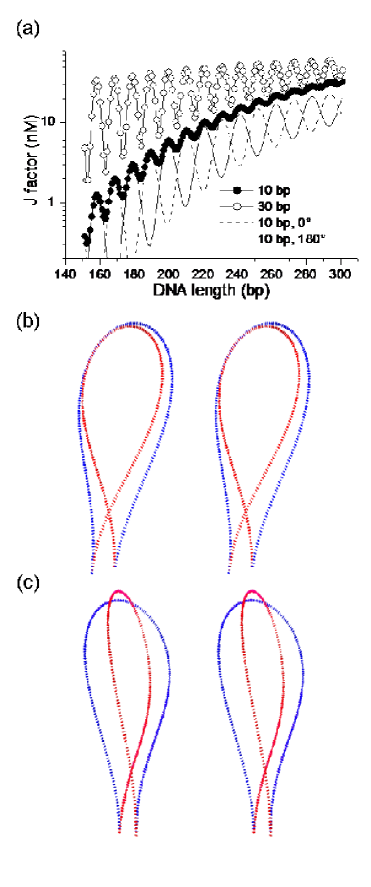
Figure 9: The DNA-length-dependent $J$-factor and loop configuration as a function of end-to-end separation (the $J$-factor is defined in section III.1). (a) The helical dependence of DNA looping is shown for values of the end-to-end separation equal to 10 bp and 30 bp. The two configurations for the 10-bp separation are obtained from corresponding configurations with zero end-to-end separation by using an iterative algorithm. Therefore the two configurations are designated by the initial configurations with phase angles $\delta=-(N-2)\tau/2+0$ ($0^{\circ}$, dashed line) and $\delta=-(N-2)\tau/2+180$ ($180^{\circ}$, solid line) as described in the text. (b) and (c) show stereo models of the two equilibrium configurations for 210-bp (b) and 215-bp (c) antiparallel DNA loops with end-to-end separation equal to 10 bp. The 210- and 215-bp DNA correspond to an adjacent peak and valley of the curve in (a), respectively. Conformations shown in blue correspond to $\delta=0$; those shown in red are for $\delta=180^{\circ}$. Note that for $N$-bp DNA, the chain contour length is equal to $(N-1)\ell_{bp}$.

Separation of the DNA ends breaks the rotational symmetry, restoring the dependence on helical twist. Figure 9a shows the $J$-factor as a function of DNA length for end-to-end distances of $10$ bp and $30$ bp. The helical dependence increases with end-to-end separation. Starting from the two loop configurations (corresponding to $\delta_{1}$ and $\delta_{2}$) with zero end-to-end distance and in-phase torsional alignment as initial configurations, two mechanical equilibrium configurations are obtained by using the iterative algorithm described in loop26 . The $J$-factor in figure 9a is the sum of separate $J$-factors calculated for the two configurations. Note that in all cases involving configurations that differ in linking number, equilibration between the two forms requires breakage of at least one of the protein-DNA interfaces. The contributions from each of these configurations are shown in detail for the case where the ends are separated by $10$ bp. Interestingly, the length dependence of $J$ computed from the individual configurations are out of phase and have a periodicity of 2 helical turns, which results from the half-twist dependence of the phase angles $\delta_{1}$ and $\delta_{2}$. However, their sum displays a periodicity of one helical turn. Figures 9 b and c show two such configurations for DNA molecules that are torsionally in-phase ($N=210$ bp) or out-of-phase ($N=215$ bp).

In the case of cyclisation, the helical-phase dependence of the $J$-factor persists at DNA lengths well beyond that corresponding to the maximum value of $J$, which lies near $500$ bp. This is clearly not the case for DNA looping. In figure 9a, the periodic dependence of $J$ on DNA length for $10$-bp end-to-end separation decays nearly to zero well before the maximum $J$ value is reached. Although the periodicity of $J$ is not attenuated quite as strongly for $30$-bp end separation, there is less than four-fold variation in the value of $J$ near $300$ bp, as opposed to the more than ten-fold variation in cyclisation $J$-factors expected in this length range. The differences between looping and cyclisation are largely due to substantial differences in the relative contributions of DNA writhe in the two processes, as discussed below.

III.6 DNA looping in synapsis

Intramolecular reactions of most site-specific recombination systems loop9 ; loop10 ; loop11 and a number of DNA restriction endonucleases such as SfiI and NgoMIV loop12 , proceed through protein-mediated intermediate structures in which a pair of DNA sites are brought together in space and the intervening DNA is looped out. The intermediate nucleoprotein complex involved in site pairing and strand cleavage (and also exchange, in the case of recombinases) is termed the synaptic complex. In these systems, two characteristic geometric parameters are of interest: the average through-space distance between the sites and the average crossing angle between the two ends of the loop, which we denote the axial angle (see section III.3). The latter quantity can be described in terms of the twist angle between the protein domains, $\tau_{PP}$ (figure 7b), and we use these terms interchangeably.

Figure 10 shows the helical dependence of looping (figure 10a) and the elastic-minimum configuration of DNA loops (figure 10b) for different values of the axial angle. The most prominent feature of these results is that the phase of the helical dependence is shifted as a function of the axial angle, characterised by a relative global shift of the curve along the $x$-axis. This implies that DNA looping does not always occur most efficiently when two sites are separated by an integral number of helical turns, as has been suggested for some simple DNA looping systems studied previously. The axial angle also globally modulates $J$-factors, which is apparent from the vertical shift in the $J$ versus length curve and effects on the amplitude of the helical dependence. The torsion-angle-independent value of $J$, averaged over a full helical turn, decreases with increasing axial angle, whereas the amplitude of the helical dependence increases. The above observations can be qualitatively explained by analogous results from DNA cyclisation. As in cyclisation, DNA forms loops most efficiently when the number of helical turns in the loop is close to an integer value. It is therefore appropriate to consider this issue in terms of the linking number for the looped conformation, $Lk$, which involves contributions from the geometries of both the protein and DNA.

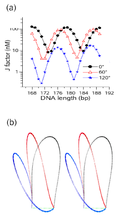
Figure 10: Dependence of the $J$-factor on axial angle (the $J$-factor is defined in section III.1, and the axial angle is defined as the average crossing angle between the two ends of the loop, see section III.3). (a) DNA-length dependence of $J$ for axial angles of $0^{\circ}$, $60^{\circ}$, and $120^{\circ}$ with the end-to-end separation set equal to 40 bp. Note that the positions of the extrema shift to the left with increasing values of the axial angle. (b) Stereo models of minimum elastic-energy conformations of 179-bp loops colour coded in accord with the corresponding axial-angle values in (a).

We define the loop helical turn $H_{t,loop}$ as the sum of the DNA twist and the twist introduced by the protein subunits, divided by $360$. Therefore, changing the twist angle, the axial angle will shift the phase of the helical dependence relative to that of the DNA alone. For a loop with $N=179$ bp and $\tau_{PP}=0$, the total twist is simply equal to that for the DNA loop. Because this loop has $17.0$ helical turns, only one loop topoisomer contributes to the $J$-factor. The value of $J$ is a local maximum at $\tau_{PP}=0$ and, as shown in figure 11a, decreases monotonically for both $\tau_{PP}>0$ and $\tau_{PP}<0$. Contributions to $J$ from other topoisomers of the $179$-bp loop are less than $5$ percent over the range $-135^{\circ}<\tau_{PP}<+120^{\circ}$. The twist for the planar equilibrium conformation of a $173$-bp loop is $16.5$ helical turns; thus there are two alternative loops that can be efficiently formed (figure 11a): either a loop with $H_{t,loop}=17.0$ and $\tau_{PP}>0$, or a loop with $H_{t,loop}=16.0$ and $\tau_{PP}<0$. The $J$ value at $\tau_{PP}=0$ is a local minimum and there is a bimodal dependence on axial angle for loops in which the DNA twist is half-integral. We investigated the phase shift of the $J$-factor and found that this quantity is a non-linear function of the axial angle. From figure 10a, the calculated phase shifts for $60^{\circ}$ and $120^{\circ}$ axial angles relative to $0^{\circ}$ are approximately $52^{\circ}$ and $103^{\circ}$, respectively. Moreover, the local maxima for the total $J$ curve for $N=173$ shown in figure 11a are located at $-58.5^{\circ}$ and $63^{\circ}$, positions that are not in agreement with predicted angle values based solely on $H_{t,loop}$ ($-166^{\circ}$ and $194^{\circ}$, respectively).

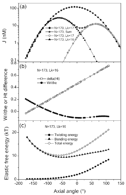
Figure 11: $J$-factor, loop-geometry parameters, and elastic-free energies as functions of axial angle; compare figure 10. (a) $J$-factor values for loop topoisomers corresponding to 179-bp and 173-bp loops in figure 10. The principal contribution to $J$ for $N=179$ bp comes from a single loop topoisomer with $Lk=17$. For $N=173$ bp, the overall $J$-factor is the sum of contributions from two loop topoisomers with $Lk$ values of 16 and 17, generating a bimodal dependence of $J$ on axial angle as described in the text. (b) Excess helical twist, $\Delta H_{t}$, and writhe of the loop formed by the $Lk=16$ topoisomer for $N=173$ bp as a function of axial angle. Excess twist is computed from the expression $H_{t,loop}-16$, where $H_{t,loop}$ is the loop helical turn value described in the text, and depends linearly on the axial angle. The writhing number of the loop was calculated using the method of Vologodskii loop28 ; loop50 . (c) Elastic-free energies of the $Lk=16$ loop topoisomer for $N=173$ bp calculated according to equation 38 of Zhang and Crothers loop26 . The individual contributions of bending and twisting energies are shown along with their sum.

These deviations can be explained by the fact that writhe makes an important contribution to the overall $Lk$ for the loop. This aspect of DNA looping is dramatically different from that in the cyclisation of small DNA molecules. The conformations of small DNA circles are close to planar and the writhe contribution is small relative to DNA twist loop26 ; loop30 ; loop44 ; loop45 . In the case of protein-mediated looping, nonzero values of the axial angle impose an intrinsically nonplanar conformation on the DNA. The relative contributions of loop writhe and twist for the $Lk=16$ topoisomer of a $173$-bp loop are shown as a function of axial angle in figure 11b.

In figure 11c, we plot the axial-angle-dependent values of the bending and twisting free energies for the $Lk=16$ topoisomer and their sum, which is the total elastic-free energy of the loop. The minimum value of the total elastic energy occurs at $\tau_{PP}=-58.5^{\circ}$, coincident with the position of the $J$-factor maximum for this topoisomer (figure 11a). This mechanical state can be achieved with very little twist deformation of the loop, but at the expense of significant bending energy. Further reduction of the axial angle requires even less twisting energy; however, the bending energy increases monotonically. In contrast, for $\tau_{PP}>-58.5^{\circ}$, somewhat less bending energy is required, but the twisting energy begins to increase significantly with increasing axial angle. Since the sense of the bending deformation for $\tau_{PP}>0$ opposes the needed reduction in loop linking number, the elastic energy cannot be decreased by increasing the axial angle. The only way that the loop geometry can compensate for this is through twist deformation. This asymmetry arises because we are considering the contribution of only one loop topoisomer to the elastic free energy.

III.7 Conclusion

The statistical-mechanical theory for DNA looping discussed above loop26 ; loop51 suggests that the helical dependence of DNA looping is affected by many factors and leads to the conclusion that whereas a positive helical-twist assay can often confirm DNA looping, a negative result cannot exclude DNA looping. Since it is difficult to explore the architecture of DNA loops with current experimental techniques, this theory will be useful for more reliably analysing DNA looping with limited experimental data. The model has advantages over previous approaches based exclusively on DNA mechanics, particularly when protein flexibility is taken into account. In these cases, entropy effects become important and are responsible for the observed decay of looping efficiency with DNA length.

IV DNA knots and their consequences: entropy and targeted knot removal

Bacterial DNA occurs largely in circular form. Notably, instead of a simply connected ring shape (the unknot), the DNA often exhibits permanently entangled states, such as catenated and knotted DNA. An example for a DNA trefoil knot is shown in figure 12. Such configurations have potentially devastating effects on the cell development. Conversely, however, knots might have designed purposes in gene regulation, separating different regions of the genome, or, alternatively, locking chemically remote parts of the genome proximate in geometrical space. In eukaryotic cells additional topological effects occur in the likely entanglement of individual chromosomes. Here, we concentrate on the prokaryotic case.

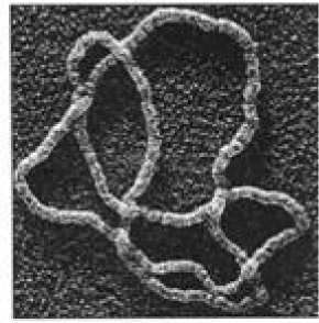
Figure 12: Electron microscope image of a DNA trefoil knot, from wassermann2 . $\copyright$ Science, with permission.

IV.1 Physiological background of knots

The discovery how one can use molecular biological tools to create knotted DNA resolved a long-standing argument against the Watson-Crick double helix picture of DNA frank , namely that the replication of DNA could not work as the opening up of the double helix would produce a superstructure such that the two daughter strands could not be separated. In fact, the topology of both ssDNA and dsDNA is continuously changed in vivo, and this can readily be mimicked in vitro, although the activity of enzymes in vivo is much more restricted than in vitro deibler ; dna_topo : Different concentrations of enzymes versus knotted DNA molecules accessible in vitro, that is, makes it possible to probe topology-altering effects by enzymes which in vivo do not contribute to such effects.

Although it would be likely with a probability of roughly $\frac{1}{2}$ that the linear DNA injected by bacteriophage $\lambda$ into its host E.coli would create a knot before cyclisation, it turned out to be difficult to detect frank . First studies therefore concentrated on the fact that under physiological conditions knots are introduced by enzymes, DNA replication and recombination, DNA repair, and topoisomerisation, using these enzymes to prove both knotting and unknotting liu ; mizuuchi ; pollock ; spengler ; wassermann ; wassermann1 ; wassermann2 . DNA-knotting is also prone to occur behind a stalled replication fork viguera ; sogo . Some of the typical topology-altering reactions undergoing in E.coli are summarised in figure 13. Knots can efficiently be created from nicked dsDNA under action of topoisomerase I at non-physiological concentrations topoknot . Another possibility is by active packaging of a DNA mutant into phage capsids arsuaga , and then denaturing the capsid proteins. Both methods produce a distribution of different knot types. They can be separated by electrophoresis electro .

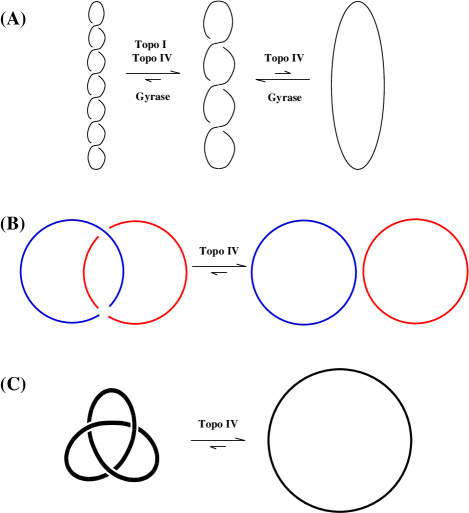
Figure 13: Enzymes changing the topology of dsDNA by cutting and pasting of one or both strands (example for E.coli ): (A) Torsional stress resulting from the Lk deficit causes the DNA double helix to writhe about itself (negative supercoiling). In E.coli , gyrase introduces negative supercoils into DNA and is countered by topoisomerase I (topo I) and topo IV, which relax negative supercoils. (B) Topo IV unlinks catenanes generated by replication or recombination in vivo. (C) Topo IV unknots DNA in vivo. After deibler .

The existence of DNA-knots has far-reaching effects on physiological processes, and knottedness of DNA has therefore to be eliminated in order to maintain proper functioning of the cell. Among other possible effects, it is immediately clear that the presence of a knot in a circular DNA impedes replication of the DNA, i.e., the full separation of the two daughter strands alberts ; frank . Moreover, even transcription is impaired portugal . The presence of knots inhibits the assembly of chromatin rodriguez , knotted chromosomes cannot be separated during mitosis alberts , and knots in a chromosome may serve as topological barriers between different sections of chromosomes, such that the genomic structural organisation is altered, and certain sections of the chromosomal DNA may no longer interact staczek . Conversely, it is conceivable that knots, analogously to protein induced DNA looping, lock remote segments of the genome close together in geometric space. Finally, knots may lead to double-strand breaks, as they weaken biopolymers considerably due to creation of localised sharp bends arai ; pieranski ; saitta ; stasiak1 as well as macroscopic lines and ropes mcnally .

Above we said that knots can be introduced, inter alia, by the different enzymes of the topoisomerase family. To remove a knot from a dsDNA, it is necessary to cut both strands, and then pass one segment through the created gap, before resealing the two open ends. In vivo, this is usually achieved by topoisomerases II and IV. A reconstruction of topo II is shown in figure 14, indicating the upper clamp holding a segment of the DNA, while the bulge-clamp introduces the cut through which the upper segment is passed. In the figure, the segment visible in the pocket of the lower clamp has already been passed through the gap. After resealing, topo II detaches. This process requires energy, provided by ATP. Notably, topo II is extremely efficient, for circular dsDNA of length $\simeq 10$ kbp it was found that topo reduced the knotted state in between 50 and 100-fold, in comparison to a ‘dumb’ enzyme, which would simply pass segments through at random rybenkov . We note that the step-wise action of topoisomerase II was recorded in a single molecule setup using magnetic tweezers stasiak ; strick . Topoisomerases are surveyed in the review of wang .

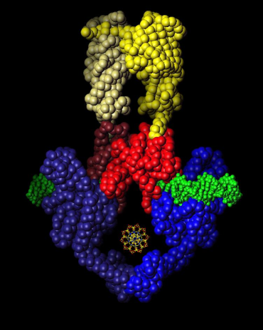
Figure 14: Topoisomerase II. This enzyme can actively change the topology of DNA by cutting the double-strand and passing another segment of double-stranded DNA through the gap before resealing it. The image depicts a short stretch of DNA (horizontally at the bulge of the enzyme, as well as another segment in the lower clamp (perpendicular to the image) after passage through the gap from the upper clamp. This mechanism makes sure that no additional strand passage through the open gap can take place berger ; wang_to . Figure courtesy James M Berger, UC Berkeley.

IV.2 Classification of knots

Knottedness can only be defined on a closed (circular) chain. This is intuitively clear as in an open linear chain a knot can always be tied, or an existing knot released. Mathematically, this means that knot invariants are only well-defined for a closed space-curve. However, a linear chain whose ends are permanently attached to one, or two walls, or whose ends are extended towards infinity, can be considered as (un)knotted in the proper mathematical sense, i.e., their knottedness cannot change. In a loser sense, we will also speak of knots on an open piece of DNA, appealing to intuition.

The classification of knots, or graphs in general, in terms of invariants can essentially be traced back to Euler, recalling his graph theoretical elaboration in connection with the Bridges of Königsberg problem euler , determining a closed path by crossing each Königsberg bridge exactly once. However, the first investigations of topological problems in modern science is most probably due to Kepler, who studied surface tiling to great detail (therefore the notion of Kepler tiling in mathematical literature) kepler . Further initial steps were due to Leibniz, Vandermonde and Gauss, in whose collection of papers drawings of various knots were found whose linking (‘Umschlingungen’=windings) number is indeed a knot invariant adams ; kauffman ; reidemeister . Gauss’ student, Listing, in fact introduced the term ‘topology’, and his work on knots may be viewed as the real starting point of knot theory listing , although his complexions number was proved by Tait not to be an invariant.

Inspired by Helmholtz’ theory of an ideal fluid and building on Listing’s early contributions to knot theory, Scotsmen and chums Maxwell, Tait and Thomson (Lord Kelvin) started to discuss the possible implications of knottedness in physics and chemistry, ultimately distilled into Thomson’s theory of vortex atoms thomson ; thomson1 . Out of this endeavour emerged Tait’s interest in knots, and he devoted most of his career on the classification of knots. Numerous charts and still unresolved conjectures on knots document his pioneering work tait ; tait1 ; tait2 ; tait3 . The studies were carried on by Kirkman and Little kirkman ; kirkman1 ; little ; little1 . A more detailed historical account of knot theory may be found in the review article by van de Griend degriend , and on the St. Andrews history of mathematics webpages.

Planar projections of knots were rendered unique by Listing’s introduction of the handedness of a crossing, i.e., the orientational information assigned to a point where in the projection two lines intersect. With this information, projections are the standard representation for knot studies. On their basis, the minimum number of crossings (‘essential crossings’) can be immediately read off as one of the simplest knot invariants. To arrive at the minimum number, one makes use of the Reidemeister moves, three fundamental permitted moves of the

Figure 15: The three Reidemeister moves. All topology-preserving moves of a knot projection can be decomposed into these three fundamental moves.

lines in a knot projection, as shown in figure 15. More complex knot invariants include polynomials of the Alexander, Kauffman and HOMFLY types adams ; kauffman ; reidemeister . Here, we will only employ the number of essential crossings as classification of knots, in particular, we do not concern ourselves with the question of degeneracy for a given knot invariant. However, the bookkeeping of knot types is vital in knot simulations.

IV.3 Long chains are almost always entangled.

During the polymerisation and final cyclisation of a polymer grown in a solvent under freely floating conditions, a knot is created with probability 1. This Frisch-Wassermann-Delbrück conjecture frisch ; delbrueck could be mathematically proved for a self-avoiding chain sumners ; pippenger , compare also vanderzande . This is consistent with numerical findings that the probability of unknot formation decreases dramatically with chain length frank3 ; volo . Indeed, recent simulations results indicate that the probability of finding the unknot in such a cyclisised polymer decays exponentially with chain length koniaris ; michels ; michels1 ; janse :

$$P_{\emptyset}(N)\propto\exp\left(-\frac{N}{N_{c}}\right).$$ (6)

However, there exist theoretical arguments and simulations results indicating that the characteristic number of monomers $N_{c}$ occurring in this relation may become surprisingly large frank2 ; grosberg4 ; klenin ; shimamura1 . The probability to find a given knot type ${\cal K}$ on random circular polymer formation has been fitted with the functional form katritch ; dobay ; shimamura1

$$P_{\cal K}(N)=a\big{(}N-N_{0}\big{)}^{b}\exp\left(-\frac{N^{c}}{d}\right),$$ (7)

where $a$, $b$, and $d$ are free parameters depending on ${\cal K}$, and $c\approx 0.18$. $N_{0}$ is the minimal number of segments required to form a knot ${\cal K}$, without the closing segment dobay . The tendency towards knotting during polymer cyclisation creates problems in industrial and laboratory processes.

IV.4 Entropic localisation in the figure-eight slip-link structure.

To obtain a feeling for how and when entropy leads to the localisation of a permanently entangled structure, we consider the simplest polymer object with non-trivial (non-unknot) geometry, the figure-eight structure (F8) displayed in figure 16. In this compound, a pair contact is enforced by a slip-link, separating off two loops in the circular polymer, such that none of the loops can fully retract, and both loops can freely exchange length among each other. We denote the loop sizes by $n$ and $N-n$, where $N$ is the (conserved) total length of the polymer chain. For such an object, we can actually perform a closed statistical mechanical analysis based on results from scaling theory of polymers, and compare the result with Monte Carlo simulations of the F8.

Figure 16: Figure-eight structure, in which a slip-link separates two loops of size $n$ and $N-n$, such that they can freely exchange length among each other, but none of the loops can completely retract from the slip-link. On the right, a schematic drawing of a slip-link, which may be thought of as a small belt buckle.

The statistical quantities that are of particular interest are the gyration radius, $R_{g}$, and the number of degrees of freedom, $\omega$ degennes . $R_{g}$, as defined in equation (61), measures the root mean squared distance of the monomers along the chain to the gyration centre, and is therefore a good measure of its extension. It can, for instance, be measured by light scattering experiment. The degrees of freedom $\omega$ count all possible different configurations of the chain. For a circular polymer (i.e., a polymer with $\mathbf{r}(0)=\mathbf{r}(N)$), the gyration radius becomes

$$R_{g}\simeq AN^{\nu}$$ (8)

with exponent $\nu=1/2$ for a Gaussian chain, and $\nu=0.588$ in the 3D excluded volume case ($\nu=3/5$ in the Flory model, and $\nu=3/4$ in 2D). Whereas in 2D this scaling contains truly a ring polymer, in 3D the exponent $\nu$ emerges from averaging over all possible topologies, and necessarily includes knots of all types duplantier1 ; deutsch ; degennes . For a circular chain, the number of degrees of freedom contains the number of all possible ways to place an $N$-step walk on the lattice with connectivity $\mu$ (e.g., $\mu=2d$ on a cubic lattice in $d$ dimensions), $\mu^{N}$, and the entropy loss for requiring a closed loop, $N^{-d\nu}$, involving the same Flory exponent $\nu$. For the Gaussian case, we recognise in this entropy loss factor the returning probability of the random walk. In the excluded volume case, $N^{-d\nu}$ is an analogous measure degennes ; grosberg ; hughes . Thus, for a circular chain embedded in $d$-dimensional space, the number of degrees of freedom is

$$\omega\simeq\mu^{N}N^{-d\nu}.$$ (9)

Let us evaluate these measures for the F8 from figure 16.

As a first approximation, consider the F8 as a Gaussian (phantom) random walk, demonstrating that, like in the charged knot case paul , entropic effects give rise to long-range interactions. The two loops correspond to returning random walks, i.e., the number of degrees of freedom for the F8 in the phantom chain case becomes degennes ; flory1 ; grosberg

$$\omega_{\rm F8,PC}\simeq\mu^{N}n^{-d/2}(N-n)^{-d/2},$$ (10)

where $d$ is the embedding dimension. We note that normalisation of this expression produces the probability density function for finding the F8 with a given loop size $\ell=na$ ($L=Na$),

$$p_{\rm F8,PC}(\ell)\simeq\mathscr{N}\ell^{-d/2}(L-\ell)^{-d/2},$$ (11)

where $\mathscr{N}$ denotes a normalisation factor. The conversion from expressing the chain size in terms of the number of monomers to its actual length is of advantage in what follows, as it allows to more easily keep track of dimensions. Here, we use the length unit $a$, which may be interpreted as the monomer size (lattice constant), or as the size of a Kuhn statistical segment.

Figure 17: Bead-and-tether chain used in Monte Carlo simulation, showing a typical equilibrium configuration for a self-avoiding chain: the localisation of the smaller loop is distinct. Note that in this 2D simulation the slip-link is represented by the three tethered black beads.

To classify different grades of localisation, we follow the convention from references slili2d ; paraknot . The average loop size $\langle\ell\rangle$ determined through $\langle\ell\rangle=\int_{a}^{L-a}\ell p(\ell)d\ell$ is trivially $\langle\ell\rangle=L/2$ by symmetry of the structure. Here, we introduce a short-distance cutoff set by the lattice constant $a$. However, as the probability density function is strongly peaked at $\ell=0$ and $\ell=L$, the two poles caused by the returning probabilities, and therefore a typical shape consists of one small (tight) and one large (loose) loop, compare figure 17. This can be quantified in terms of the average size of the smaller loop,

$$\langle\ell\rangle_{<}\equiv 2\int_{a}^{L/2}\ell p(\ell)d\ell\,.$$ (12)

In $d=2$, we obtain

$$\langle\ell\rangle_{<}\sim\frac{L}{|\log(a/L)|},$$ (13)

such that with the logarithmic correction the smaller loop is only marginally smaller than the big one. In contrast, one observes weak localisation

$$\langle\ell\rangle_{<}\sim a^{1/2}L^{1/2}$$ (14)

in $d=3$, in the sense that the relative size $\langle\ell\rangle_{<}/L$ tends to zero for large chains. By comparison, for $d>4$ one encounters $\langle\ell\rangle_{<}\sim a$, corresponding to strong localisation, as the size of the smaller loop does not depend on $L$ but is set by the short-distance cutoff $a$. Above four dimensions, excluded volume effects become negligible, and therefore both Gaussian and self-avoiding chains are strongly localised in $d\geq 4$.

To include self-avoiding interactions, we make use of results for general polymer networks obtained by Duplantier duplantier ; duplantier1 , which are summarised in the appendix at the end of this review. In terms of such networks, our F8-structure corresponds to the following parameters: the number ${\cal N}=2$ of polymer segments with lengths $s_{1}=\ell=na$ and $s_{2}=L-\ell=(N-n)a$, forming ${\cal L}=2$ physical loops, connected by $n_{4}=1$ vertex of order four. By virtue of equation (79), the number of configurations of the F8 with fixed $\ell$ follows the scaling form

$$\omega_{\rm F8}(\ell)\simeq\mu^{L}(L-\ell)^{\gamma_{\rm F8}-1}{\cal X}_{\rm F8}\left(\frac{\ell}{L-\ell}\right),$$ (15)

with the configuration exponent $\gamma_{\rm F8}=1-2d\nu+\sigma_{4}$. In the limit $\ell\ll L$, the contribution of the large loop in equation (15) should not be affected by a small appendix, and therefore should exhibit the regular Flory scaling $\sim(L-\ell)^{-d\nu}$ kafri ; kafri1 ; duplantier3 . This fixes the scaling behaviour of the scaling function ${\cal X}_{\rm F8}(x)\sim x^{\gamma_{\rm F8}-1+d\nu}$ in this limit ($x\to 0$ in dimensionless variable $x$), such that

$$\omega_{\rm F8}(\ell)\simeq\mu^{L}(L-\ell)^{-d\nu}\ell^{-c},\quad\ell\ll L,$$ (16)

where $c=-(\gamma_{\rm F8}-1+d\nu)=d\nu-\sigma_{4}$. Using $\sigma_{4}=-19/16$ and $\nu=3/4$ in $d=2$ duplantier ; duplantier1 , we obtain

$$c=43/16=2.6875,\quad d=2.$$ (17)

In $d=3$, $\sigma_{4}\approx-0.48$ schaefer ; kafri ; kafri1 and $\nu\approx 0.588$, so that

$$c\approx 2.24.$$ (18)

In both cases the result $c>2$ enforces that the loop of length $\ell$ is strongly localised in the sense defined above. This result is self-consistent with the a priori assumption $\ell\ll L$. Note that for self-avoiding chains, in $d=2$ the localisation is even stronger than in $d=3$, in contrast to the corresponding trend for ideal chains.

We performed Monte Carlo (MC) simulations of the 2D figure-eight structure, in which the slip-link was represented by three tethered beads enforcing a sliding pair contact such that the loops cannot fully retract (see figure 18). We used a 2D hard core bead-and-tether chain with 512 monomers, starting off from a symmetric initial condition with $\ell=L/2$. Self-crossings were prevented by keeping a maximum bead-to-bead distance of 1.38 times the bead diameter, and a maximum step length of 0.15 times the bead diameter. As shown in figure 19, the size distribution for the small loop can be fitted to a power law with exponent $c=2.68$ in good agreement with equation (17).

Figure 18: Monte Carlo simulation of an F8-structure in 2D: loop sizes $\ell$ and $L-\ell$ as a function of Monte Carlo steps for a chain with 512 monomers. The symmetry breaking after the symmetric initial condition is distinct.

Figure 19: Power-law fit to the probability density function of the smaller loop. The fit produces a slope of -2.68, in excellent agreement with the calculated value.

An experimental study of entropic tightening of a macroscopic F8-structure was reported in reference bennaim . There, a granular chain consisting of hollow steel spheres connected by steel rods was once twisted and then put on a vibrating table. From digital imaging, the distribution of loop sizes could be determined and compared to a power-law with index 43/16 as calculated for the 2D excluded volume chain. The agreement was found to be consistent bennaim .

IV.5 Simulations of entropic knots in 2D and 3D.

Much of our knowledge about the interaction of knots with thermal fluctuations is based on simulations of knotted chains. Before going further into the theoretical modelling of knotted chains, we report some of the results based on simulations studies of both Gaussian and self-avoiding walks. Such simulations either start with a given knot configuration and then perform moves of specific segments, each time making sure that the topology is preserved; or, each new configuration emanates from a new random walk, whose correct topology may be checked by calculating the corresponding knot invariant, usually the Alexander polynomial, and created configurations that do not match the desired topology are discarded. We note that it is of lesser significance that knot invariants such as the Alexander polynomials in fact are no longer unique for more complex knots, because for typical chain lengths with the highest probability simpler knots are created, for which the invariants are unique. For more details we refer to the works quoted below.

In fact, the fixed topology turns out to have a highly non-trivial effect on chains without self-excluded volume. As conjectured in descloizeaux , a Gaussian circular chain, whose permitted set of configurations is restricted to a fixed topology, will exhibit self-avoiding behaviour. This was proved in a numerical analysis in deutsch . The required number of monomers to reach this self-avoiding exponent was estimated to be of the order of 500. Keeping this non-trivial scaling of a Gaussian chain at fixed topology in mind, knot simulations on the basis of phantom Gaussian chains were performed in dobay1 , always making sure that the configurations taken into the statistics fulfil the desired knot topology.

The dependence of the gyration radius $R_{g}$ on the knot type was investigated for simpler knots in 3D in reference janse . On the basis of the expansion

$$R_{g}^{2}\simeq A_{\cal K}\Big{(}1+B_{\cal K}N^{-\Delta}+C_{\cal K}N^{-1}+o(1/N)\Big{)}N^{2\nu_{\cal K}},$$ (19)

including a confluent correction janse ; leguillou ; zinn in comparison to the standard expression (8), it was found that the Flory exponent $\nu_{\cal K}$ is independent of the knot type ${\cal K}$ and has the 3D value $0.588$. This was interpreted via a localisation of knots such that the influence of tight knots on $R_{g}$ is vanishingly small. In fact, $\Delta$ is of the order of $0.5$ according to the investigations in references leguillou ; zinn ; janse1 ; li . Based on longer chains in comparison to reference janse , the study of orlandini thus corroborates the independence of $\nu_{\cal K}\approx 0.588$ of the knot type ${\cal K}$. In recent AFM experiments analysing single DNA knots, the Flory scaling $R_{g}\simeq N^{\nu}$ was confirmed for both simple and complex knots valle .

For the number of degrees of freedom $\omega_{\cal K}$, it was found for the form

$$\omega_{\cal K}\simeq A_{\cal K}N^{\alpha_{\cal K}-2}\mu_{\cal K}^{N}\left(1+\frac{B_{\cal K}}{N^{\Delta_{\cal K}}}+\ldots\right)$$ (20)

with confluent corrections, that while for the unknot with $\alpha_{\emptyset}\approx 0.27$ expression (20) is consistent with the standard result (9) ($[0.27-2]/3\approx-0.58\approx\nu$), for prime knots $\alpha_{\cal K}=\alpha_{\emptyset}+1$, and for composite knots with $N_{f}$ prime components,

$$\alpha_{\cal K}=\alpha_{\emptyset}+N_{f}.$$ (21)

This finding is in agreement with the view that each prime component of a knot ${\cal K}$ is tightly localised and statistically able to move around one central loop, each prime component counting an additional factor $N$ of degrees of freedom. The fact that for a chain of finite thickness the size of the big central loop is in fact diminished by the size of the tight knot is a confluent effect, such that the confluent exponent $\Delta$ should be related to the size distribution of the knot region. Not surprisingly, the connectivity factor $\mu_{\cal K}\approx 4.68$ was found to be independent of ${\cal K}$, assuming the standard value for a cubic lattice guttmann . Also the amplitude $A_{\cal K}$ and the exponent $\Delta_{\cal K}$ of the confluent correction turned out to be ${\cal K}$-independent. We note that a similar analysis in (pseudo) 2D also strongly points towards tight localisation of the knot guitter .

In contrast to the above results, 3D simulations undertaken in quake (also compare quake1 ) show the dependence

$$R_{g}\simeq N^{3/5}C^{-4/15}$$ (22)

of the gyration radius on the knot type, characterised by the number $C$ of essential crossings. $R_{g}$, that is, decreases as a power-law with $C$, where the exponent $-4/15=1/3-\nu$ quake . The functional form (22)) was derived from a Flory-type argument for a polymer construct of $C$ interlocked loops of equal length $N/C$ by arguing that each loop occupies a volume $\simeq(N/C)^{3\nu}$, and the volume of the knot is given by $V\simeq C(N/C)^{3\nu}$ (i.e., assuming that due to self-avoiding repulsion the volume of individual loops adds up to the total volume). Equation (22) then follows immediately. This model of equal loop sizes is equivalent to a completely delocalised knot. It may therefore be speculated, albeit rather long chain sizes of up to 400 were used, whether the numerical algorithm employed for the simulations in quake causes finite-size effects that, in turn, prevent a knot localisation. We note that the Flory-type scaling assumed to derive expression (22) is consistent with a modelling brought forward in reference grosberg2 , in which the knot is quantified by the aspect ratio in a configuration corresponding to a maximally inflated tube with the given topology (i.e., a state corresponding to complete delocalisation). In reference quake , the temporal relaxation behaviour of a given knot was also studied. While regular Rouse behaviour was found for the case of the unknot, the knotted chains displayed somewhat surprising long time contributions to the relaxation time spectrum treloar ; ward ; ferry ; erman , a phenomenon already pointed out by de Gennes within an activation argument to create free volume in a tight knot in order to move along the chain degennesma . Note that relatively lose knots in shorter chains do not appear to exhibit such extremely long relaxation time behaviour lai1 .

Simulation of a 3D knot with varying excluded volume showed, if only the excluded volume becomes large enough, the gyration radius of the knot is independent of the knot type shimamura . The picture of tight knots is further corroborated in the study by Katritch et al. using a Gaussian chain model with fixed topology to demonstrate that the size distribution of the knot is distinctly peaked at rather small sizes katritch .

Apart from determining the statistical quantities $R_{g}$ and $\omega_{\cal K}$ from simulations, there also exist indirect methods for quantifying the size of the knot region in a knotted polymer. One such method is to confine an open chain containing a knot between two walls, and measuring the finite size corrections of the force-extension curve due to the knot size. This is based on the idea that the gyration radius for a system depending on more than one length scale (i.e., apart from the chain length $N$) shows above mentioned confluent corrections, such that farago

$$R_{g}=AN^{\nu}\Phi\left(\frac{N_{0}}{N},\frac{N_{1}}{N},\ldots\right)\simeq AN^{\nu}\Big{(}1-BN^{-\Delta}\Big{)}$$ (23)

when only the largest correction is considered, and in 3D $\Delta\approx 0.5$ is supposed to be universal leguillou ; zinn ; janse1 ; li . If this leading correction is due to the argument $N_{0}/N$ in the scaling function $\Phi$, the length scale $N_{0}$ depends on $N$ through the scaling $N_{0}\sim N^{t}$ with $\Delta=1-t$. From Monte Carlo simulations of a bead and tether chain model, it could then be inferred that the size of the knot scales like farago

$$N_{k}\sim N^{t},\quad t=0.4\pm 0.1$$ (24)

This, in turn, enters the force-extension curve $f^{\prime}=G(R^{\prime})$ with the dimensionless force $f^{\prime}=fAN^{\nu}/(k_{B}T)$ and distance $R^{\prime}=R/(AN^{\nu})$ of the walls, in the form with confluent correction

$$f^{\prime}\simeq G(R^{\prime})\Big{(}1+g(R^{\prime})N^{-\Delta}\Big{)}.$$ (25)

From the simulation, $t=0.4$ corresponds to the best data collapsing, assuming the validity of the scaling arguments. An argument in favour of this approach is the consistency of the exponent $t=0.4$ with the inferred $\Delta=0.6$, which is close to the known value. Note that the force-extension of a chain with a slip-link was discussed in reference pull and shown that a loop separated off by a slip-link is confined within a Pincus-de Gennes blob. We also note that results corresponding to delocalisation in force-size relations were reported in sheng ; sheng1 . An entropic scale was conceived in roya : Separating two chains with fixed topology but allowing them to exchange length (e.g., through a small hole in a wall) would enable one to infer the localisation behaviour of a knot by comparing the equilibrium balance of this knot with a slip-link construct of known degrees of freedom until the average length on both sides coincides. The preliminary results in roya are shadowed by finite-size effects of the accessible system size, as limited by computation power. The analysis in reference marcone of a self-avoiding polygon model uses the method of closure of a short fragment of the knot and subsequent determination of its Alexander polynomial to obtain the scaling exponent $t=0.75$; in a second variant, the authors find a consistent result by a variant of the knot scale method. Another recent study uses a more realistic model for a polymer chain, namely, a simplified model of polyethylene; with up to 1000 monomers in the simulation, the exponent $t\approx 0.65$ is found (and delocalisation is obtained in the dense phase) virnau .

Thus, there exist simulations results pointing in both directions, knot localisation and delocalisation. As the latter may be explained by finite size effects, it seems likely that (at least simple) knots in 2D and 3D localise in the sense that the knot region occupies a portion of the chain that is significantly smaller in comparison to the entire chain. In particular, this would imply that the average size of the knot region $\langle\ell\rangle$ scales with the chain length $Na$ with an exponent less than one, such that

$$\lim_{N\to\infty}\frac{\langle\ell\rangle}{Na}=0.$$ (26)

Below, we show from analytical grounds that such a localisation is a natural consequence of interactions of a chain of fixed topology with fluctuations. We note, however, that conclusive results for knot localisation may in fact come from experiments: Manipulation of single chains such as DNA can be performed for rather long chains, making it possible to reach beyond the finite-size corrections inherent in, e.g., the force-extension simulations mentioned above. The aforementioned AFM studies on single DNA knots indeed reveal knot localisation of flattened knots valle ; due to experimental limitations, presently only one DNA length was investigated, such that the scaling exponent $t$ currently cannot be obtained.

Before proceeding to these analytical approaches, we note that there have also been performed simulations of knotted chains under non-dilute conditions stella ; orlanddense . In (pseudo) 2D, these have found delocalisation of the knot, i.e., $\lim_{N\to\infty}\langle\ell\rangle/N=const$. We come back to these simulations below in connection with the modelling of dense and $\Theta$-knots.

IV.6 Flattened knots in dilute and dense phases.

Analytically, knots are a hard problem to tackle. Statistical mechanical treatments of permanently entangled polymers are so difficult to treat since topological restrictions cannot be formulated as a Hamiltonian problem but appear as hard constraints partitioning the phase space degennes ; grosberg ; vilgis ; kholodenko . A segment of a 3D knot, in other words, can move without feeling the constraints due to the non-trivial topology of a knotted state, until it actually collides with another segment. The accessible phase space of degrees of freedom is therefore characterised by inequalities.

Consequently, only a relatively small range of problems have been treated analytically, starting with the seminal papers by Edwards edwards1 ; edwards2 , in which he considers the classification of topological constraints in polymer physics. De Gennes addressed the problem of tight knot motion along a polymer chain using scaling arguments for the activation of free length inside the knot region, producing a double-exponential expression for the corresponding time scale degennesma , which might explain the extreme long-time contributions in the relaxation time spectrum of permanently entangled polymers doi ; treloar ; ward ; erman ; ferry . Some analytical results were obtained for a pair, or an ‘Olympic’ gel of entangled polymer rings, see for instance, otto ; otto1 ; vilgis1 ; ferrari ; ferrari1 . In a mean field approach based on the Kauffman invariant the entropy of knots was investigated in references grone ; grone1 ; grone2 . Similarly, some statistical properties of random knot diagrams were investigated in nechaev ; nechaev1 . However, some insight can be gained on the basis of phenomenological models, which we will come back to below. Here, we continue with an analytical study of flat knots.

One possibility to treat knotted polymer chains analytically is to confine the degrees of freedom of the knot to motion in 2D, only. The knot, that is, is preserved, as at the crossings the chain is allowed to form an over-/underpassing, while the rest of the knot is confined to 2D. Such a confinement can in fact be experimentally realised in various ways. Thus, the chain can be confined between two close-by glass slabs, as demonstrated in craighead ; it can be pressed flat on a surface by gravitation or similar forces, for instance in macroscopic systems bennaim ; bennaim1 ; the chain can be adhesively bound to a membrane and still reach configurational equilibrium, as experimentally shown for DNA in references valle ; maier . Or it can be adsorbed to a mica surface either by APTES coating or by providing bivalent Mg ions in solution, as shown in figure 20. From such flat knots as discussed in the remainder of this section, we will be able to infer certain generic features also for 3D knots.

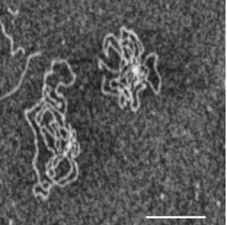
Figure 20: AFM tapping-mode images of flattened, complex DNA-knots with approximately 30-40 essential crossings, see valle . The substrate surface used is AP-mica (freshly cleaved mica reacted with an amino terminal silane to obtain a positively charged surface). The DNA knots used are extracted from bacteriophage P4; the DNA is a 11.4 kbp molecule (with a 1.4 kbp deletion resulting in a final length of 10 kbp) which has two cohesive ends. They are not covalently closed, thus no supercoiling is present. The knot adsorbed out of the 3D bulk on to the surface is strongly trapped, i.e., the knot is ‘projected’ onto the surface without any equilibration. The knot appears rather delocalised. Courtesy F. Valle and G. Dietler.

A flat knot therefore corresponds to a polymer network in 2D, but the orientation of the crossings is preserved, such that the network graph actually coincides with a typical knot projection kauffman ; reidemeister ; adams , as shown in figure 21 on the left. This projection of the trefoil, and similar projections for all knots, displays the knot with the essential crossings. A flat knot can, in principle acquire an arbitrary number of crossings by Reidemeister moves; for instance, the bottom left segment of the flat trefoil can slide under the vicinal segment, creating a new pair of vertices, and so on. However, we suppose that such transient additional loops are sufficiently short-lived so that we can neglect them in our analysis. Then, we can apply results from scaling analysis of polymer networks of the most general type shown in figure 79, see the primer in the appendix. We note that from the Monte Carlo simulations we performed it may be concluded that such additional vertices can in fact be neglected.

IV.6.1 Flat knots in dilute phase.

We had previously found that for the F8-structure the probability density function for the size of each loop is peaked at $\ell\to 0$ and $\ell\to L$. From the scaling analysis for self-avoiding polymer networks, we concluded strong localisation of one subloop. For more complicated structures, the joint probability to find the individual segments with given lengths $s_{i}$ is expected to peak at the edges of the higher-dimensional configuration hyperspace. Some analysis is necessary to find the characteristic shapes. Let us consider here the simplest non-trivial knot, the (flat) trefoil knot $3_{1}$ shown in figure 21.

Figure 21: Flat trefoil knot with segment labels. On the right, a schematic representation of a localised flat trefoil with one large segment is shown.

Each of the three crossings is replaced with a vertex with four outgoing legs, and the resulting network is assumed to separate into a large loop and a multiply connected region which includes the vertices. Let $\ell=\sum_{i=1}^{5}s_{i}$ be the total length of all segments contained in the multiply connected knot region. Accordingly, the length of the large loop is $s_{6}=L-\ell$.

In the limit $\ell\ll L$, the number of configurations of this network can be derived in a similar way as in the scaling approach followed for the F8. This procedure determines the concrete behaviour of the scaling form

$$\omega_{\rm III}\simeq\mu^{L}{\cal W}_{\rm III}\left(L-\ell,\ell,\frac{s_{1}}{\ell},\frac{s_{2}}{\ell},\frac{s_{3}}{\ell},\frac{s_{4}}{\ell}\right)$$ (27)

including the scaling function ${\cal W}$ that depends on altogether six arguments. The index III is chosen according to figure 22, where the flat trefoil configuration in the dense phase appears at position III of the scheme (explained below). After some manipulations, the number of degrees of freedom yields in the form slili2d

$$\omega_{\text{III}}(\ell,L)\sim\mu^{L}(L-\ell)^{-d\nu}\ell^{-c},$$ (28)

with the scaling exponent

$$c=-(\gamma_{\text{III}}-1+d\nu)-m,\qquad m=4.$$ (29)

Here, $m=4$ corresponds to the number of independent integrations over the segments $s_{i}$ ($i=1,\ldots,4$) of the knot region, as we only retain the cumulative size $\ell=\sum_{i=1}^{5}s_{i}$ of the knot region. Putting numerical values, we find $c=65/16$, i.e., strong localisation.

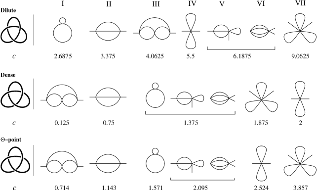
Figure 22: Hierarchy of the flat trefoil knot $3_{1}$. Upper row: dilute phase. Middle row: $\Theta$-phase. Bottom row: dense phase. To the left of each row, the trefoil projection is shown. It splits up into the hierarchies of configurations, with exponents $c$ below each contraction. The small protruding legs represent the big central loop, compare, for instance, figure 21 on the right with position III of the top row. See text for details.

However, some care is necessary in performing these integrations, since the scaling function ${\cal W}_{\rm III}$ may exhibit non-integrable singularities if one or more of the arguments $s_{i}/\ell$ tend to $0$. The geometries corresponding to these limits (edges of the configuration hyperspace) represent contractions of the original trefoil network ${\cal G}_{\text{III}}$ in the sense that the length of one or more of the segments $s_{i}$ is of the order of the short-distance cutoff $a$. If such a short segment connects different vertices, they cannot be resolved on larger length scales, but appear as a single, new vertex. Thus, each contraction corresponds to a different network ${\cal G}$, which may contain a vertex with up to eight outgoing legs. For the flat trefoil knot, there exist six different contractions, as grouped in figure 22 around the original flat trefoil at position III. As an example, in the top row of figure 22 contraction VI follows from the original trefoil III if the uppermost segment becomes very small, and similarly the network VII emanates from contraction VI if one of the four symmetric segments becomes very small. For each of these networks, one can calculate the corresponding exponent $c$ in a similar way as above, leading to the general expression

$$c=2+\sum_{N\geq 4}n_{N}\left\{\frac{N}{2}\Big{(}d\nu-1\Big{)}+\Big{(}|\sigma_{N}|-d\nu\Big{)}\right\}.$$ (30)

The $\sigma_{N}$ are given in equation (80). In figure 22, the various contractions are arranged in increasing exponent $c$.

Our scaling analysis relies on an expansion in $a/\ell\ll 1$, and the values of $c$ determine a sequence of contractions according to higher orders in $a/\ell$: The smallest value of $c$ corresponds to the most likely contraction, while the others represent corrections to this leading scaling behaviour, and are thus less and less probable (see figure 22). To lowest order, the trefoil behaves like a large ring polymer at whose fringe the point-like knot region is located. At the next level of resolution, it appears contracted to the figure-eight shape ${\cal G}_{\mathrm{I}}$. For more accurate data, the higher order shapes II to VII may be found with decreasing probability. Interestingly, the original uncontracted trefoil configuration ranks third in the hierarchy of shapes.

These predictions were checked by MC simulations with the same conditions as described above, to prevent intersection. The flat trefoil knot was prepared from a symmetric, harmonic 3D representation with 512 monomers, which was collapsed and then kept on a hard wall by the “gravitational” field $V=-k_{B}Th/h^{*}$ perpendicular to the wall, where $h$ is the height of a monomer, and $h^{*}$ was set to 0.3 times the bead diameter. Configurations corresponding to contraction I are then selected by requiring that besides a large loop, they contain only one segment larger than a preset cutoff length (taken to be 5 monomers), and similarly for contraction II. The size distributions for such contractions, as well as for all possible knot shapes are shown in figure 23.

Figure 23: Power law tails in probability density functions for the size $\ell$ of tight segments: As defined in the figure, we show results for the smaller loop in a figure-eight structure, the overall size of the trefoil knot, as well as the two leading contractions of the latter.

The tails of the distributions are indeed consistent with the predicted power laws, although the data (especially for contraction II) is too noisy for a definitive statement.

Our scaling results pertain to all flat prime knots. In particular, the dominating contribution for any prime knot corresponds to the figure-eight contraction ${\cal G}_{\text{I}}$, as equation (30) predicts a larger value of the scaling exponent $c$ for any network ${\cal G}$ other than ${\cal G}_{\text{I}}$. Accordingly, figure 24 demonstrates

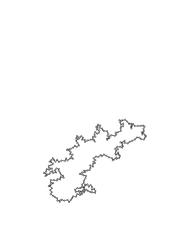
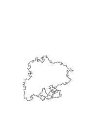
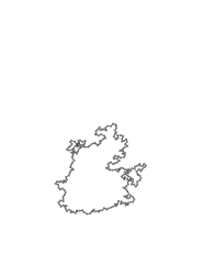
Figure 24: Typical configurations of 256-mer chains for the trefoil $3_{1}$, the prime knot $8_{19}$, and the composite knot $3_{1}$#$3_{1}$ consisting of two trefoils, in $d=2$. The initial conditions were symmetric in all cases.

the tightness of the prime knot $8_{19}$. Composite knots, however, can maximise the number of configurations by splitting into their prime factors as indicated in figure 24 for $3_{1}$#$3_{1}$. Each prime factor is tight and located at the fringe of one large loop, and accounts for an additional factor of $L$ for the number of configurations as compared to a ring of length $L$ without a knot. Indeed, this gain in entropy leads to the tightness of knots. Flat knots can experimentally be produced by ‘projecting’ a dilute 3D knot from the bulk onto a mica surface, on which the knot is adsorbed. Variation of the ionic strength in the solution determines whether the knot is going to be strongly trapped on the surface such that, once captured on the surface, it is completely immobilised (small ionic strength); or whether the adsorption is weaker such that the knot can (partially) equilibrate while being confined to 2D, i.e., equilibrate as a flat knot. Figure 20 shows a strongly trapped complex knot, whereas figure 25 depicts a weakly adsorbed simple knot, compare valle .

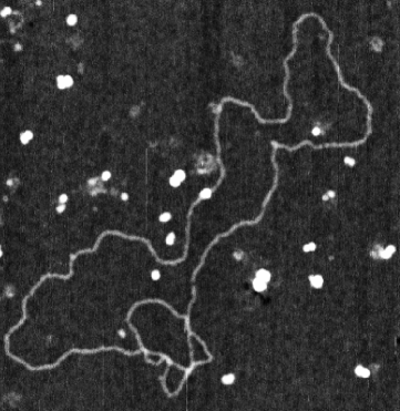
Figure 25: Flat knot imaged by AFM, similar to the one shown in figure 20. However, this knot is rather simple (likely a trefoil) and was allowed to relax while attaching to freshly cleaved mica in the presence of bivalent Mg counterions. Courtesy E. Ercolini, J. Adamcik, and G. Dietler. Note the close resemblance to the trefoil configuration shown in figure 24.

IV.6.2 Flat knots under $\Theta$ and dense conditions.

In many situations, polymer chains are not dilute. Polymer melts, gels, or rubbers exhibit fairly high densities of chains, and the behaviour of an individual chain in such systems is significantly different compared to the dilute phase degennes ; doi ; erman . Similar considerations apply to biomolecules: in bacteria, the gyration radius of the almost freely floating ring DNA may sometimes be larger than the cell radius itself. Moreover, under certain conditions, there is a non-negligible osmotic pressure due to vicinal layers of protein molecules, which tends to confine the DNA walter ; vasilevskaya ; lerman . In protein folding studies, globular proteins in their native state are often modelled as compact polymers on a lattice (see garel for a recent review).

A polymer is considered dense if, on a lattice, the fraction $f$ of occupied sites has a finite value $f>0$. This can be obtained by considering a single polymer of total length $L$ inside a box of volume $V$ and taking the limit $L\to\infty$, $V\to\infty$ in such a way that $f=L/V$ remains finite duplantier2 ; duplantier3 ; jacobsen . Alternatively, dense polymers can be obtained in an infinite volume through the action of an attractive force between monomers. Then, for temperatures $T$ below the collapse (Theta) temperature $\Theta$, the polymers collapse to a dense phase, with a density $f>0$, which is a function of $T$ duplantier3 ; duplantier4 ; owczarek ; owczarek1 . For a dense polymer in $d$ dimensions, the exponent $\nu$, defined by the radius of gyration $R_{g}\sim L^{\nu}$, becomes $\nu=1/d$. The limit $f=1$ is realised in Hamiltonian paths, where a random walk visits every site of a given lattice exactly once duplantier7 ; kondev . Dense polymers may be related to 2D vesicles and lattice animals (branched polymers) fisher ; seno ; dekeyser ; cardy .

As studied in reference dense , the value of the exponent $c$ for the 2D dense F8 is (compare to the appendix)

$$c=-\gamma_{\rm F8}=11/8=1.375,$$ (31)

implying that the smaller loop is weakly localised. This means that the probability for the size of each loop is peaked at $\ell=0$ and, by symmetry, at $\ell=L$. An analogous reasoning for the 2D F8 at the $\Theta$ point gives

$$c=11/7=1.571.$$ (32)

In both cases the smaller loop is weakly localised in the sense that $\langle l\rangle_{<}/L\to 0$. Figure 26 shows

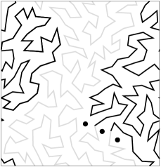
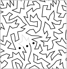
Figure 26: Symmetric ($\ell=L/2=128$) initial configuration of a 2D dense F8 (left) and equilibrium configuration (right) with periodic boundary conditions. The two different grey values correspond to the two subloops created by the slip-link. The slip-link itself is represented by the three (tethered) black dots.

the symmetric initial and a typical equilibrium configuration for periodic boundary conditions obtained from Monte Carlo (MC) simulations, see reference dense for details. In figure 26, the lines represent the bonds (tethers) between the monomers (beads, not shown here). The three black dots mark the locations of the tethered beads forming the slip-link in 2D. The initial symmetric configuration soon gives way to a configuration with $\ell\ll L$ on approaching equilibrium. Figure 27 shows the development of this symmetry breaking as a function of the number of MC steps. We note, however, that the fluctuations of the loop sizes in the “stationary” regime appear to be larger in comparison to the dilute case studied in reference paraknot , compare figure 18. We checked that for densities (area coverage) above 40% the scaling behaviour becomes independent of the density. (The above simulation results correspond to a density of 55%.) The size distribution data is well fitted to a power law (for over 1.5 decades with 1024 monomers), and the corresponding exponent with 512 and 1024 monomers in figure 27 is in good agreement with the predicted value (31).

For our MC analysis, we again used a hard core bead-and-tether chain, in which self-crossings were prevented by keeping a maximum bead-to-bead distance of 1.38 times the bead diameter, and a maximum step length of 0.15 times the bead diameter. To create the dense F8 initial condition, a free F8 is squeezed into a quadratic box with hard walls. This is achieved by starting off from the free F8, surrounding it by a box, and turning on a force directed towards one of the edges. Then, the opposite edge is moved towards the centre of the box, and so on. During these steps, the slip-link is locked, i.e., the chain cannot slide through it, and the two loops are of equal length during the entire preparation. Finally, when the envisaged density is reached, the hard walls are replaced by periodic boundary conditions, and the slip-link is unlocked. After each step, the system is allowed to relax for times larger than the localisation times occurring at the main stage of the run.

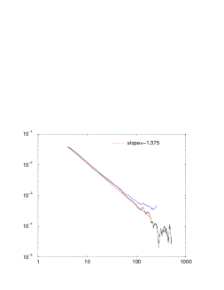
Figure 27: The loop size probability distribution $p(\ell)$ at $\rho=55\%$ area coverage, for the F8 with 512 (top) and 1024 (bottom) monomers. The power law with with the predicted exponent $c=1.375$ in equation (31) is indicated by the dotted line.

A similar analysis as for the dense/$\Theta$-F8 structure and the dilute flat trefoil above, reveals the number of degrees of freedom for the flat dense trefoil in the form dense

$$\omega_{3}(\ell,L)\sim\omega_{0}(L)\ell^{-c}$$ (33)

with $c=-\gamma_{3}-m$, where $\gamma_{3}=-33/8$ from equation (82) in the appendix (${\cal L}=4$, $n_{4}=3$) and $m=4$ is the number of independent integrations over chain segments. Thus, $c=1/8<1$ which implies that the dense 2D trefoil is delocalised. As above, we have to consider the various possible contractions of the flat knot. For dense polymers, the present scaling results show that both the original trefoil shape ($c=1/8<1$, see above) and position II ($c=3/4<1$) are in fact delocalised and represent equally the leading scaling order (cf. top part of figure 22). The F8 is only found at the third position and is weakly localised ($c=11/8>1$). In an MC simulation of the dense 2D trefoil, we predict that one mainly observes delocalised shapes corresponding to the original trefoil and position II in figure 22, and further, with decreasing probability, the weakly localised F8 and the other shapes of the hierarchy (top part) in figure 22.

These predictions are consistent with the numerical simulations of reference stella , who observe that the mean value of the second largest segment of the simulated 2D dense trefoil configurations grows linearly with $L$, and conjecture the same behaviour also for the other segments, corresponding to the delocalisation of the trefoil obtained above.

An analogous reasoning can be applied to the 2D trefoil in the $\Theta$ phase. We find that in this case that the leading shape is again the original (uncontracted) trefoil, with $c=5/7<1$. This implies that the 2D trefoil is delocalised also at the $\Theta$ point. All other shapes are at least weakly localised, and subdominant to the leading scaling order represented by the original trefoil. The resulting hierarchy of shapes is shown in figure 22 (bottom part).

IV.7 3D knots defy complete analytical treatment.

As already mentioned, 3D knots correspond to a problem involving hard constraints that defy a closed analytical treatment. It may be possible, however, that by a suitable mapping to, for instance, a field theory, an analytical description may be found. This may in fact be connected to the study of knots in diagrammatic solutions in high energy physics gambini . There exists a fundamental relation between knots and gauge theory as knot projections and Feynman graphs share the same basic ingredients corresponding to a Hopf algebra kauffman . However, up to now no such mapping has been found, and a theoretical description of 3D knots based on first principles is presently beyond hope. To obtain some insight into the statistical mechanical behaviour of knotted chains, one therefore has to resort to simulations studies or experiments. In addition, a few phenomenological models for both the equilibrium and dynamical behaviour of knots have been suggested such as in references quake ; slili3d ; lai1 ; sheng1 ; sheng ; grosberg1 ; grosberg2 ; grosberg4 .

When discussing numerical knot studies, we already mentioned the Flory-type model brought leading to equation 22 quake ; quake1 . One may argue that the differences in the knot size for the different knot types corresponding to the same $C$ may be included in the prefactor, that is independent of the chain length $N$. Obviously, this model of equal loop sizes is equivalent to a completely delocalised knot. This statement is in fact equivalent to another Flory-type approach to knotted polymers reported in grosberg2 . In this model, the knot is thought of as an inflatable tube: for a very thin tube diameter, the tube is equivalent to the original knot conformation; inflating the tube more and more will increasingly smoothen out the shape until a maximally inflated state is reached. The knot is then characterised by the aspect ratio

$$p=\frac{L}{D}\,\,,\,\mbox{therefore}\,\,1\leq p\leq N,$$ (34)

between length $L$ and maximum tube diameter $D$. It appears that $p$ is a (weak) knot invariant, and can be used to characterise the gyration radius of the knot. It is clear that, by construction, the aspect ratio described a totally delocalised knot, and indeed it turns out that in good solvent, the gyration radius shows the dependence $R_{g}\simeq AN^{3/5}\tau^{1/5}p^{-4/15}$, where $\tau$ is the (dimensionless) deviation from the $\Theta$ temperature grosberg2 . Obviously, the aspect ratio appears to be proportional to the number of essential crossings in comparison to expression (22). We note that similar considerations are employed in reference grosberg1 , including a comparison to the entropy of a tight knot, finding comparable entropic likelihood. The modelling based on the aspect ratio $p$ is further refined in grosberg4 .

Knot localisation is a subtle interplay between the degrees of freedom of one big loop, and the internal degrees of freedom of the various segments in the knot region. Under localisation, the number of degrees of freedom

$$\omega\simeq\mu^{N}N^{1-d\nu}$$ (35)

includes an additional factor $N$ from the knot region encircling the big loop. For flat knots, the competition between the single big loop and the knot region is indeed won by the big loop. In the case of 3D knots, this balance is presently not resolved for knots of all complexity. Probably only detailed simulations studies of higher order knots will make it possible to decide for the various models of 3D knots. Major contributions are also expected from single molecule experiments, for instance, from force-extension measurements along the lines of the simulations study in farago , the advantage of experiments being the fact that it should be possible to go towards rather high chain lengths that are inaccessible in simulations. To overcome similar difficulties in the context of the entropic elasticity for rubber networks, Ball, Doi, Edwards and coworkers replaced permanent entanglements by slip-links edwards2a ; edwards2b ; edwards2c ; edwards2d . Gaussian networks containing slip-links have been successful in the prediction of important physical quantities of rubber networks erman , and they have been used to study a small number of entangled chains sommer . In a similar fashion, one may investigate the statistical behaviour of single polymer chains in which a fixed topology is created by a number of slip-links. Such ‘paraknots’ can be studied analytically using the Duplantier scaling results paraknot . As mentioned previously, knowledge of the statistical behaviour of paraknots can be used to create a knot scale for calibrating the degrees of freedom of real knots, and therefore also important to understand or design indirect experiments on knot entropy, such as by force-extension measurements pull . Paraknots may also be useful in the design of entropy-based functional molecules hame_cpl ; meamb_ctn .

V DNA breathing: local denaturation zones and biological implications

”A most remarkable physical feature of the DNA helix, and one that is crucial to its functions in replication and transcription, is the ease with which its component chains can come apart and rejoin. Many techniques have been used to measure this melting and reannealing behaviour. Nevertheless, important questions remain about the kinetics and thermodynamics of denaturation and renaturation and how these processes are influenced by other molecules in the test tube and cell” kornberg . This remarkable quotation, despite 30 years old, still summarises the challenge of understanding local and global denaturation of DNA, in particular, its dynamics. In this section, we report recent findings on the spontaneous formation of intermittent denaturation zones within an intact DNA double helix. Such denaturation bubbles fluctuate in size by (random) motion of the zipper forks relative to each other. The opening and subsequent closing of DNA bubbles is often called DNA breathing.

Figure 28: Fraction $\theta_{h}$ of double-helical domains within the DNA as a function of temperature. Schematic representation of $\theta_{h}(T)$, showing the increased formation of bubbles and unzipping from the ends, until full denaturation has been reached.

V.1 Physiological background of DNA denaturation

The Watson-Crick double-helix is the thermodynamically stable configuration of a DNA molecule under physiological conditions (normal salt and room/body temperature). This stability is effected (a) by Watson-Crick H-bonding, that is essential for the specificity of base-pairing, i.e., for the key-lock principle according to which the nucleotide Adenine exclusively binds to Thymine, and Guanine only to Cytosine. Base-pairing therefore guarantees the high level of fidelity during replication and transcription. (b) The second contribution to DNA-helix stability comes from base-stacking between neighbouring bps: through hydrophobic interactions between the planar aromatic bases, that overlap geometrically and electronically, the bp stacking stabilises the helical structure against the repulsive electrostatic force between the negatively charged phosphate groups located at the outside of the DNA double-strand. While hydrogen bonds contribute only little to the helix stability, the major support comes from base-stacking kornberg ; delcourt .

The quoted ease with which its component chains can come apart and rejoin, without damaging the chemical structure of the two single-strands, is crucial to many physiological processes such as replication via the proteins DNA helicase and polymerase, and transcription through RNA polymerase. During these processes, the proteins unzip a certain region of the double-strand, to obtain access to the genetic information stored in the bases in the core of the double-helix kornberg ; revzin ; watsoncrick . This unzipping corresponds to breaking the hydrogen bonds between the bps. Classically, the so-called melting and reannealing behaviour of DNA has been studied in solution in vitro by increasing the temperature, or by titration with acid or alkali. During thermal melting, the stability of the DNA duplex is related to the content of triple-hydrogen-bonded G-C bps: the larger the fraction of G-C pairs, the higher the required melting temperature or pH value. Thus, under thermal melting, dsDNA starts to unwind in regions rich in A-T bps, and then proceeds to regions of progressively higher G-C content kornberg ; delcourt . Conversely, molten, complementary chains of single-stranded DNA (ssDNA) begin to reassociate and eventually reform the original double-helix under incubation at roughly 25^∘ below the melting temperature $T_{m}$ kornberg . The relative amount of molten DNA in a solution can be measured by UV spectroscopy, revealing large changes in absorption in the presence of perturbed base-stacking wartell . Careful melting studies allow one to obtain accurate values for the stacking energies of the various combinations of neighbouring bps, a basis for detailed thermodynamic modelling of DNA-melting and DNA-structure per se blake ; blossey . In fact, thermal melting data have been successfully used to identify coding sequences of the genome due to the different G-C content yeramian ; yeramian1 ; carlon .

Complementary to thermal or pH induced denaturation, dsDNA can be driven toward denaturation mechanically, by applying a tensional stress along the DNA in an optical tweezer trap williams . As shown in figure 29, the force per extension increases in worm-like chain fashion, until a plateau at approximately 65 pN is reached. This plateau is sometimes interpreted as new DNA configuration, the S form busta . By a series of experiments, it appears more likely that the plateau corresponds to the mechanical denaturation transition williams1 . To first order, the effect of the longitudinal pulling translates into an external torque $\mathfrak{T}$, whose effect is a decrease in the free energy for melting a bp:

$$\Delta G_{F}=\Delta G_{F=0}-\mathfrak{T}\theta_{0},$$ (36)

where $\theta_{0}=2\pi/10.35$ is the twist angle per bp of the double helix hwa .

Figure 29: Overstretching of double-stranded DNA. The black curve shows the typical force-extension behaviour of DNA following the rapid worm-like chain increase until at around 65 pN a plateau is reached. Crossing of the plateau corresponds to progressive mechanical denaturation. See text for details. Figure courtesy Mark C. Williams.

An important application of thermal DNA melting is the Polymerase Chain Reaction (PCR). In PCR, dsDNA is melted at elevated temperatures into two strands of ssDNA. By lowering the temperature in a solution of invariable primers and single nucleotides, each ssDNA is completed to dsDNA by the key-lock principle of base-pairing pcr ; pcrrev . By many such cycles, of the order of $10^{9}$ copies of the original DNA can be produced within the range of hours. Again, the error rate due to the underlying biochemistry can be considered negligible for most purposes. In particular, from the viewpoint of polymer physics/chemistry, the obtained sample is monodisperse and free of parasitic reactions, creating (almost) ideal samples for physical studies, in particular, as any designed sequence of bases can be custom-made in modern molecular biology labs snustad .

While the double-helix is the thermodynamically stable configuration of the DNA molecule below $T_{m}$ (at non-denaturing pH), even at physiological conditions there exist local denaturation zones, so-called DNA-bubbles, predominantly in A-T-rich regions of the genome wartell ; poland . Driven by ambient thermal fluctuations, a DNA-bubble is a dynamical entity whose size varies by thermally activated zipping and unzipping of successive bps at the two forks where the ssDNA-bubble is bordered by the dsDNA-helix. This incessant zipping and unzipping leads to a random walk in the bubble-size coordinate, and to a finite lifetime of DNA-bubbles under non-melting conditions, as eventually the bubble closes due to the energetic preference for the closed state wartell ; poland . DNA-breathing typically opens up a few bps gueron ; krueger . It has been demonstrated recently that by fluorescence correlation methods the fluctuations of DNA-bubbles can be explored on the single molecule level, revealing a multistate kinetics that corresponds to the picture of successive zipping and unzipping of single bps. At room temperature, the characteristic closing time of an unbounded bp was found to be in the range 10 to 100 $\mu$sec corresponding to an overall bubble lifetime in the range of a few msec altan . The multistate nature of the DNA-breathing was confirmed by a UV-light absorption study zocchi . The zipping dynamics of DNA is also investigated by NMR methods nmr ; nmr1 ; nmr2 , revealing considerably shorter time scales than the fluorescence experiments. An interesting finding from NMR studies is the dramatically different denaturation dynamics in B’ DNA, where more than three AT bps occur in a row russu . It is conceivable that fluorescence correlation and NMR probe different levels of the denaturation dynamics. Our analysis of the single DNA fluorescence data reported below demonstrates that, albeit the much longer time scale, the dependence of the measured autocorrelation function on the stacking along the sequence is very sensitive, and agrees well with the quantitative behaviour predicted from the stability data.

The presence of fluctuating DNA-bubbles is essential to the understanding of the binding of single-stranded DNA binding proteins (SSBs) that selectively bind to ssDNA, and that play important roles in replication, recombination and repair of DNA kornberg1 . One of the key tasks of SSBs is to prevent the formation of secondary structure in ssDNA alberts ; snustad . From the thermodynamical point of view one would therefore expect SSBs to be of an effectively helix-destabilising nature, and thus to lower $T_{m}$ vonhippel . However, it was found that neither the gp32 protein from the T4 phage nor E.coli SSBs do vonhippel ; vonhippel1 ; rich . An explanation to this apparent paradox was suggested to consist in a kinetic block, i.e., a kinetic regulation such that the rate constant for the binding of SSBs is smaller than the one for bubble closing vonhippel1 ; rich1 . This hypothesis could recently be verified in extensive single molecule setups using mechanical overstretching of dsDNA by optical tweezers in the presence of T4 gene 32 protein pant ; pant1 ; pant2 , as detailed below.

V.2 The Poland-Scheraga model of DNA melting

The most widely used approach to DNA melting in bioinformatics is the statistical, Ising model-like Poland-Scheraga model (sometimes also referred to as Bragg-Zimm model) and its variations poland ; cantor ; wartell ; see also kafri ; kafri1 ; richard ; hanke . It defines the partition function $\mathscr{Z}$ of a DNA molecule in a grand canonical picture with arbitrary many bubbles. For simplicity, we will restrict the following discussion to a single bubble. Below the melting temperature $T_{m}$, the one bubble picture is a good approximation: due to the high energy cost of bubble initiation, the distance between bubbles on a DNA molecule is large, and bubbles behave statistically independently. In typical experimental setups for measuring the bubble dynamics (see below), the used DNA construct is actually designed to host an individual bubble. For a homopolymer stretch of double-stranded DNA with 400 bps, figure 30 shows the probabilities to find zero, one or, or two bubbles as a function of the Boltzmann factor $u=\exp(\Delta G/RT)$ for denaturation of a single bp. Even at the denaturation transition $\Delta G=0$, it is quite unlikely to find two bubbles simultaneously.

Figure 30: Probability of having 0, 1, or 2 bubbles as a function of $u$ for a DNA region of chain length 400 bps. The cooperativity parameter was $\sigma_{0}=10^{-3}$ and the loop correction exponent c=1.76 (see text).

The free energy $\Delta G$ to break an individual bp are constructed as follows. We mention two different approaches. Common for both is the Poland-Scheraga construction of the partition function. We start with the case that a linear DNA molecule denatures from one of its ends. The corresponding partition function is poland ; wartell

$$\mathscr{Z}_{\mathrm{end}}(m)=\prod_{x=1}^{m}e^{\Delta G_{x,x+1}/RT}$$ (37)

where $m$ is the number of broken bps, and $\Delta G_{x,x+1}$ is the stacking free energy for disruption of the bp at position $x$ measured from the end of the DNA. The notation explicitly refers to the stacking between the bp at $x$ and $x+1$. The first closed bp is located at $x=m+1$. For a homonucleotide, $\Delta G_{x,x+1}=\Delta G$, while for a given sequence of bps, there come into play the different stacking energies for the possible combinations of pairs of bps in sequence The stacking energies $\Delta G_{x,x+1}$ have the following contributions.

The more traditional way to determine the stacking interactions is by fit of bulk melting curves of DNA constructs containing exclusively pairs of the specific bp-bp combination such as $(\mathrm{AT/TA})_{n}$ (see, e.g., santalucia ; delcourt and references therein). The free energy used in this automated fit procedure using the MELTSIM algorithm blake ,

$$\Delta G^{\mathrm{Mix}}_{x,x+1}=\Delta H^{\mathrm{ST}}_{x,x+1}-T\Delta S_{x,x+1},$$ (38)

combines the stacking enthalpy difference $\Delta H^{\mathrm{ST}}_{x,x+1}$ for both hydrogen bond and actual stacking energies, and the entropy difference $\Delta S_{x,x+1}$ chosen to explicitly depend on the nature of the broken bp. A recent alternative to determine the stability parameters of DNA was developed in the group of Frank-Kamenetskii, leading to the free energy krueger

$$\Delta G^{\mathrm{Sep}}_{x,x+1}=\Delta G^{\mathrm{ST}}_{x,x+1}+\Delta G^{\mathrm{HB}}_{x}$$ (39)

where the Gibbs free energies $\Delta G^{\mathrm{ST}}_{x,x+1}$ and $\Delta G^{\mathrm{HB}}_{x}$ measure the stacking of bps $x$ and $x+1$ and the hydrogen bonding of bp $x$ including the entropy release on disruption. Note that $\Delta G^{\mathrm{HB}}_{x}$ is chosen such that it only depends on the broken bp and has two values for AT and GC bps, irrespective of the orientation (3’ or 5’). The stacking free energies $\Delta G^{\mathrm{ST}}$ were determined from denaturation at a DNA nick and show a pronounced asymmetry between AT/TA and TA/AT bonds krueger . For an end-denaturing DNA both descriptions are equivalent (though somewhat different when one puts numbers), as the breaking of each bp involves the disruption of one hydrogen bonds of bp $x$ and one stacking with its neighbour.

The difference between the two approaches becomes apparent when we consider the initiation of a bubble, i.e., a denatured coil enclosed by intact double-helix. Now, the partition function for a bubble with left fork position at $x_{L}$ and consisting of $m$ broken bps,

$$\mathscr{Z}_{\mathrm{mid}}(x_{L},m)=\Lambda\Sigma(m)\prod_{x=x_{L}}^{x_{L}+m}e^{\Delta G_{x,x+1}/RT},$$ (40)

differs from (37) in three respects: (i) While the bubble consists of $m$ molten bps, $m+1$ stacking interactions need to be broken to create two boundaries between intact double-strand and the single-strand in the bubble; the extra stacking interaction is effectively incorporated into $\Lambda$. (ii) The polymeric nature of the flexible single-stranded bubbles involves the entropy loss factor $\Sigma(m)=1/(m+D)^{c}$ with critical exponent $c$ and the parameter $D$ to take care of finite size effects richard ; blake ; fixman ; (iii) the factor $\Lambda$: In the standard notation, $\Lambda\equiv\sigma_{0}=\exp(-F_{s}/RT)\simeq 10^{-4}-10^{-5}$ lazurkin ; blake ; wartell ; poland , while according to krueger , $\Lambda=\xi\simeq 10^{-3}$ is called the ring factor. Interestingly, the cooperativity parameter $\sigma_{0}$ is of the order of what corresponds to the singular unbalanced stacking enthalpy for breaking the first bp to initiate the bubble. The new stability data lead to a more pronounced asymmetry in opening probabilities between different bp-bp combinations. The analysis in references tobias_prl ; tobias_long demonstrates that the parameters from krueger appear to support better the biological relevance of the TATA motif in natural sequences, that is, show a more pronounced simultaneous opening probability for the TATA motif.

As demonstrated for the autocorrelation function measuring the breathing dynamics in figure 32, the description in terms of the partition function $\mathscr{Z}$ based on the stability parameters from krueger reproduces the experimental data well. The analysis in tobias_prl ; tobias_long also indicates that the accuracy of the model predictions for the bubble dynamics is rather sensitive to the parameters. It is therefore conceivable that improved fluorescence measurement of the bubble dynamics may be employed to obtain accurate DNA, stability parameters, complementing the more traditional melting, NMR, and gel electrophoresis bulk methods. It should be noted that the dynamics is strongly influenced by local deviations from the B configuration of the DNA double helix. Thus, in local stretches of more than three AT bps in sequence, the B’ structure is assumed, leading to pronouncedly different zipping dynamics russu .

Two major questions remain in the thermodynamic formulation of DNA denaturation and its dynamics. Namely, the exact origin of the bubble initiation factor $\sigma_{0}$ (or, alternatively, the ring factor $\xi$ from krueger ), and a method to properly calibrate the zipping rate $k$. The factor $\sigma_{0}$ is related to the entropic imbalance on opening the first bp of a bubble: While this requires the breaking of two stacking interactions, only one bp has access to an increased amount of degrees of freedom. Still, these degrees of freedom must be influenced by the fact that the single open bp is coupled to two zipper forks. Currently, $\sigma_{0}$ remains a fit parameter. The exact value of the zipping rate $k$ remains open. While NMR experiments indicate much faster rates in the nanosecond range ($\simeq 10^{8}\mbox{ sec}^{-1}$), the fluorescence correlation measurements produce values in the microsecond range ($\simeq 10^{4}-10^{5}\mbox{ sec}^{-1}$). This large discrepancy may be based on the fact that both methods have different sensitivity to the amplitude of intra-bp separation. Currently, $k$ is taken as a fit parameter. In the analysis in tobias_prl ; tobias_long , we use the stacking parameters from krueger including the value of the ring factor $\xi$, so that $k$ (a shift along the logarithmic abscissa) is the only adjustable parameter.

It has been under debate what exact value should be taken for the critical exponent $c$ entering in the entropy loss factor for a denaturation bubble. This is connected to the fact that $c>2$ would imply a first order denaturation transition on melting, while $1<c<2$ would stand for a second order transition fisher ; richard . Speculations about a possible first order transition are connected to the rather distinct spikes in the differential melting curves wartell . Theoretical polymer physics approaches to explain a $c>2$ are either based on the inclusion of polymeric self-avoidance interactions of the bubble with the remainder of the chain kafri ; or built on a directed polymer model garel1 . Despite the elegance of both approaches, it is an open question how truly they represent the detailed denaturation behaviour of real DNA hame_comment ; somendra_comment . Applying the MELTSIM algorithm to typical sequences, it was found that there is a connection between the fit result for the cooperativity parameter $\sigma_{0}$, whose value is reduced from $\approx 10^{-5}$ to $\approx 10^{-3}$ by assuming $c=2.12$ instead of $1.76$ blossey . Below the melting transition, the typical bubble size is only a few bps, and in that regime the polymeric treatment of the loop entropy loss is of approximative nature. Indeed, in the analysis of krueger no entropy loss due to polymer ring formation was included. For the breathing dynamics, we include $c$, to cover higher temperatures with somewhat larger bubbles, but find no significant change in the behaviour between $c<2$ and $c>2$, as long as the exponent is sufficiently close to 2. We therefore use the value $c=1.76$, that is consistent with the traditional data fits employed in the determination of the stacking parameters.

V.3 Fluctuation dynamics of DNA bubbles: DNA breathing

Below the melting temperature $T_{m}$, DNA bubbles are intermittent, i.e., they form spontaneously due to thermal fluctuations, and after some time close again. DNA-breathing can be thought of as a biased random walk in the phase space spanned by the bubble size $m$ and its position denoted, e.g., by the left zipper fork position $x_{L}$ tobias_prl ; tobias_long . The bubble creation can be viewed as a nucleation process landau , whereas the bubble lifetime corresponds to the survival time of the first passage problem of relaxing to the $m=0$ state after a random walk in the $m>0$ halfspace hame_jpa ; tobias_jpc ; tobias_prl ; tobias_long ; tobias_pre . Bubble breathing on the single DNA-bubble level was measured by fluorescence correlation spectroscopy in altan . This technique employs a designed stretch of DNA, in which weaker AT bps form the bubble domain, that is clamped by stronger GC bonds. In the bubble domain, a fluorophore-quencher pair is attached. Once the bubble is created, fluorophore and quencher are separated, and fluorescence occurs. A schematic of this setup is shown in figure 31.

Figure 31: Clamped DNA domain with internal bps $x=1$ to $M$, statistical weights $u_{\rm hb}(x)$, $u_{\rm st}(x)$, and tag position $x_{T}$. The DNA sequence enters through the statistical weights $u_{\rm st}(x)$ and $u_{\rm hb}(x)$ for disrupting stacking and hydrogen bonds respectively. The bubble breathing process consists of the initiation of a bubble and the subsequent motion of the forks at positions $x_{L}$ and $x_{R}$. See tobias_long for details.

The zipper forks move stepwise $x_{L/R}\rightarrow x_{L/R}\pm 1$ with rates $\mathsf{t}^{\pm}_{L/R}(x_{L/R},m)$. We define for bubble size decrease

$$\mathsf{t}^{+}_{L}(x_{L},m)=\mathsf{t}^{-}_{R}(x_{L},m)=k/2\qquad(m\geq 2)$$ (41)

for the two forks. The rate $k$ characterises a single bp zipping. Its independence of $x$ corresponds to the view that bp closure requires the diffusional encounter of the two bases and bond formation; as sterically AT and GC bps are very similar, $k$ should not significantly vary with bp stacking. The rate $k$ is the only adjustable parameter of our model, and has to be determined from experiment or future MD simulations. The factor $1/2$ is introduced for consistency tobias_jpc ; tobias_pre ; tobias_prl ; tobias_long ; tobias_leif . Bubble size increase is controlled by

$$\mathsf{t}_{L}^{-}(x_{L},m) = ku_{\rm st}(x_{L})u_{\rm hb}(x_{L})s(m)/2,$$

$$\mathsf{t}_{R}^{+}(x_{L},m) = ku_{\rm st}(x_{R}+1)u_{\rm hb}(x_{R})s(m)/2,$$ (42)

for $m\geq 1$, where $s(m)=\{(1+m)/(2+m)\}^{c}$. Finally, bubble initiation and annihilation from and to the zero-bubble ground state, $m=0\leftrightarrow 1$ occur with rates

$$\mathsf{t}_{G}^{+}(x_{L}) = k\xi^{\prime}s(0)u_{\rm st}(x_{L}+1)u_{\rm hb}(x_{L}+1)u_{\rm st}(x_{L}+2)$$

$$\mathsf{t}_{G}^{-}(x_{L}) = k.$$ (43)

The rates $\mathsf{t}$ fulfil detailed balance conditions. The annihilation rate $\mathsf{t}_{G}^{-}(x_{L})$ is twice the zipping rate of a single fork, since the last open bp can close either from the left or right. Due to the clamping, $x_{L}\geq 0$ and $x_{R}\leq M+1$, ensured by reflecting conditions $\mathsf{t}_{L}^{-}(0,m)=\mathsf{t}_{R}^{+}(x_{L},M-x_{L})=0$. The rates $\mathsf{t}$ together with the boundary conditions fully determine the bubble dynamics.

In the FCS experiment fluorescence occurs if the bps in a $\Delta$-neighbourhood of the fluorophore position $x_{T}$ are open altan . Measured fluorescence time series thus correspond to the stochastic variable $I(t)$, that takes the value 1 if at least all bps in $[x_{T}-\Delta,x_{T}+\Delta]$ are open, else it is 0. The time averaged ($\overline{\,\,\cdot\,\,}$) fluorescence autocorrelation

$$A_{t}(x_{T},t)=\overline{I(t)I(0)}-\overline{I(t)}^{2}$$ (44)

for the sequence AT9 from altan are rescaled in figure 32.

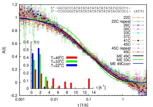
Figure 32: Time-dependence of the autocorrelation function $A_{t}(x_{T},t)$ for the sequence AT9 measured in the FCS setup of reference altan at 100mM NaCl. The full lines show the result from the master equation, based on the DNA stability parameters from Krueger et al. krueger . The inset shows the broadening of the relaxation time spectrum with increasing temperature.

We note that an alternative method to obtain precise DNA stability data may be provided by a DNA construct with two AT-rich zones between which a shorter GC-rich bridge is located. The first passage problem corresponding to bubble merging at temperatures between the melting temperatures of the AT and GC zones was recently calculated hansen , and provides the framework for modified fluorescence correlation setups similar to the one from reference altan .

V.4 Probabilistic modelling—the master equation (ME)

DNA breathing is described by the probability distribution $P(x_{L},m,t)$ to find a bubble of size $m$ located at $x_{L}$ whose time evolution follows the ME tobias_jpc ; tobias_pre ; tobias_prl ; tobias_long ; tobias_leif

$$\frac{\partial}{\partial t}P(x_{L},m,t)=\mathbb{W}P(x_{L},m,t).$$ (45)

The transfer matrix $\mathbb{W}$ incorporates the rates $\mathsf{t}$. Detailed balance guarantees equilibration toward $\lim_{t\to\infty}P(x_{L},m,t)=\mathscr{Z}(x_{L},m)/\mathscr{Z}$, with $\mathscr{Z}=\sum_{x_{L},m}\mathscr{Z}(x_{L},m)$ vankampen . The ME and the explicit construction of $\mathbb{W}$ are discussed at length in references tobias_jpc ; tobias_long . Eigenmode analysis and matrix diagonalisation produces all quantities of interest such as the ensemble averaged autocorrelation function

$$A(x_{T},t)=\langle I(t)I(0)\rangle-(\langle I\rangle)^{2}.$$ (46)

$\langle I(t)I(0)\rangle$ is proportional to the survival density that the bp is open at $t$ and that it was open initially tobias_prl ; tobias_long .

In figure 32 the blue curve shows the predicted behaviour of $A(x_{T},t)$, calculated for $T=49^{\circ}$C with the parameters from krueger . As in the experiment we assumed that fluorophore and quencher attach to bps $x_{T}$ and $x_{T}+1$, that both are required open to produce a fluorescence signal. From the scaling plot, we calibrate the zipping rate as $k=7.1\times 10^{4}/$s, in good agreement with the findings from reference altan . The calculated behaviour reproduces the data within the error bars, while the model prediction at $T=35^{\circ}$C shows more pronounced deviation. Potential causes are destabilising effects of the fluorophore and quencher, and additional modes that broaden the decay of the autocorrelation. The latter is underlined by the fact that for lower temperatures the relaxation time distribution $f(\tau)$, defined by $A(x_{T},t)=\int\exp(-t/\tau)f(\tau)d\tau$, becomes narrower (figure 32 inset). Deviations may also be associated with the correction for diffusional motion of the DNA construct, measured without quencher and neglecting contributions from internal dynamics oleg1 . Indeed, the black curve shown in figure 32 was obtained by a 3% reduction of the diffusion time; see details in tobias_long .

A remark on a prominent alternative approach to DNA breathing appears in order. This is the Peyrard Bishop Dauxois (PBD) model peyrard ; dauxois based on the set of Langevin equations peyrard_cm

$$m\frac{d^{2}y_{n}}{dt^{2}} = -\frac{dV(y_{n})}{dy_{n}}-\frac{dW(y_{n+1},y_{n})}{dy_{n}}-\frac{dW(y_{n},y_{n-1})}{dy_{n}}$$ (47)

$$-m\gamma\frac{dy_{n}}{dt}=\xi_{n}(t).$$

Here, $V(y_{n})=D_{n}\left[\exp(-a_{n}y_{n})-1\right]^{2}$ is a Morse potential for the hydrogen bonding, $D_{n}$ and $a_{n}$ assuming two different values for AT and GC bps; $W(y,y^{\prime})=\frac{k}{2}\left[1+\rho\exp\{-\beta(y+y^{\prime})\}\right](y-y^{\prime})^{2}$ is a nonlinear potential to include bp-bp stacking interactions between adjacent bps $y$ and $y^{\prime}$. The parameters $k$, $\rho$, $\beta$, $\gamma$, and $m$ are invariant of the sequence. Usually, the stochastic equations (47) is integrated numerically peyrard_cm . Due to its formulation in terms of a set of Langevin equations, the DPB model is very appealing, and it is a useful model to study some generic features of DNA denaturation. The disadvantage of the current formulation of the DBP model is the fact that it does not include enough parameters to account for the known independent stability constants of double stranded DNA (in fact, only two parameters are allowed to vary with the sequence, in contrast to the 12 independent parameters needed to fully describe the bp stacking and hydrogen bonding krueger ). Moreover, there appear to be certain ambiguities in the proper formulation of boundary conditions in the stochastic integration the_prl_footnote , and also with respect to the interpretation of the biological relevance and computational limitations of the PBD model peyrard_comment . The master equation and Gillespie approach brought forth in references tobias_jpc ; tobias_pre ; tobias_prl ; tobias_long ; tobias_leif bridges the gap between the thermodynamic data for the bp stacking and hydrogen bonding obtained by various experimental methods, and the dynamical nature of DNA breathing. It is hoped that both dynamic models will synergetically be developed further and eventually lead to a better understanding of DNA denaturation fluctuations.

V.5 Stochastic modelling—the Gillespie algorithm

Figure 33: Time series of single bubble-breathing dynamics for $\sigma_{0}=10^{-3}$, $M=20$, and (a) $u=0.6$ and (b) $u=0.9$. The lower panel shows a zoom-in of how single bubbles of size $m(t)$ open up and close.

Despite its mathematically simple form, the master equation (45) needs to be solved numerically by inverting the transfer matrix tobias_jpc ; tobias_long . Moreover, it produces ensemble-averaged information. Given the access to single molecule data, it is of relevance to obtain a model for the fully stochastic time evolution of a single DNA-bubble, providing a description for pre-noise-averaged quantities such as the step-wise (un)zipping. With this scope, we introduced a stochastic simulation scheme for the (un)zipping dynamics, using the Gillespie algorithm to update the state of the system by determining (i) the random time between individual (un)zipping events, and (ii) which reaction direction (zipping, $\leftarrow$, or unzipping, $\rightarrow$) will occur suman . This scheme is efficient computationally, easy to implement, and amenable to generalisation.

To define the model, we denote a bubble state of $m$ broken bps by the occupation numbers $b_{m}=1$ and $b_{m^{\prime}}=0$ ($m^{\prime}\neq m$). The stochastic simulation then corresponds to the nearest-neighbour jump process

$$b_{0}\rightleftarrows b_{1}\rightleftarrows\ldots\rightleftarrows b_{m}\rightleftarrows\ldots\rightleftarrows b_{M-1}\rightleftarrows b_{M},$$ (48)

with reflecting boundary conditions at $b_{0}$ and $b_{M}$. Each jump away from state $b_{m}$ occurs after a random time $\tau$, and in random direction to either $b_{m-1}$ or $b_{m+1}$, governed by the reaction probability density function gillespie ; gillespie1

$$P(\tau,\mu)=\mathsf{t}^{\mu}(m)e^{-\left(\mathsf{t}^{+}(m)+\mathsf{t}^{-}(m)\right)\tau},$$ (49)

where $\mu\in\{+,-\}$ denotes the unzipping ($+$) or zipping ($-$) of a bp, and the jump rates $\mathsf{t}^{\pm}(m)$ are defined below. From the joint probability density function (49), the waiting time probability density function that a jump away from $b_{m}$ occurs is given by $\psi(\tau)=\sum_{\mu}P(\tau,\mu)$, i.e., it is Poissonian. The probability that the bubble size does not change in the time interval $[0,t]$ is given by $\phi(t)=1-\int_{0}^{t}\psi(\tau)d\tau$. The fork position $x_{L}$ (and thereby the sequence of bps) is straightforwardly incorporated tobias_prl ; tobias_long .

We start the simulations from the completely zipped state, $b_{0}=1$ at $t=0$, and measure the bubble size at time $t$ in terms of $m(t)=\sum_{m=0}^{M}mb_{m}(t)$. The time series of $m(t)$ for a single stochastic realization is shown in figure 33. It is distinct that the bubble events are very sharp (note the time windows of the zoom-ins), and most of the time the zero-bubble state $b_{0}$ prevails due to $\sigma_{0}\ll 1$. Moreover, raising the temperature increases the bubble size and lifetime, as it should. By construction of the simulation procedure, it is guaranteed that an occupation number $b_{m}=1$ ($m\neq 0$) corresponds to exactly one bubble.

In a careful analysis, it was shown that the stochastic simulation method provides accurate information of the statistical quantities of the bubble, such as opening probability and autocorrelation function suman . It can therefore be used to obtain the same information as the master equation with the advantage of also giving access to the noise in the system. With the Gillespie technique, we also obtained the data points in the graphs in this section.

V.6 Bacteriophage T7 promoter sequence analysis.

An example from the analysis of the promoter sequence

$$\begin{array}[]{l}\mbox{\small{{\color[rgb]{1,1,1}AAAA}1{\color[rgb]{1,1,1}AAAAAAAAAAAAAAAAAA}20}}\\[-2.84544pt] \mbox{\small{{\color[rgb]{1,1,1}AAAA}|{\color[rgb]{1,1,1}AAAAAAAAAAAAAAAAAA}|{\color[rgb]{1,1,1}AAAAAAAAA}{\color[rgb]{1,1,1}AAA}}}\\[-2.84544pt] \mbox{\small{5'-aTGACCAGTTGAAGGACTGGAAGTAATACGACTC}}\\ \mbox{\small{{\color[rgb]{1,1,1}AAA}AG}{\color[rgb]{1,0,0} {TATA}}{GGGACAATGCTTAAGGTCGCTCTCTAGGAg-3'}}\\[-2.84544pt] \mbox{\small{{\color[rgb]{1,1,1}AAAAA}|{\color[rgb]{1,1,1}AAA}| {\color[rgb]{1,1,1}AAAAAAAAAAAAAAAAAAAAAAAAAA}|{\color[rgb]{1,1,1}AAA}}}\\[-2.84544pt] \mbox{\small{{\color[rgb]{1,1,1}AAAAA}{\color[rgb]{1,0,0}38}{\color[rgb]{1,1,1}AA}{\color[rgb]{0,0,1}41}{\color[rgb]{1,1,1}AAAAAAAAAAAAAAAAAAAAAAAAAA}68{\color[rgb]{1,1,1}AAA}}}\end{array}$$ (50)

of bacteriophage T7 is shown in figure 34 tobias_prl . It depicts the time series of $I(t)$ for the tag positions $x_{T}=38$ at the beginning of TATA, and $x_{T}=41$ at the first GC bp after TATA. It is distinct how frequent bubble events are in TATA in comparison to the vicinal GC-rich domain (note that AT/TA bps are particularly weak krueger ). This is quantified by the waiting time density $\psi(\tau)$, whose characteristic time scale is more than an order of magnitude longer for the $x_{T}=41$ position. In contrast, we observe almost identical behaviour for the bubble survival density $\phi(\tau)$. Due to the proximity of $x_{T}=41$ to TATA, the typical bubble sizes for both tag positions are similar, and therefore the relaxation time. However, as shown in figure 34 bottom, the variation of the mean lifetime obtained from the master equation is quite small (within a factor 2) for the entire sequence. The latter graph also shows the insignificant variation according to the earlier stability parameters by Blake et al. blake .

The results summarised in figure 34 and further studies in tobias_prl ; tobias_long may indicate that it is not solely the increased opening probability at the TATA motif, as studied in choi . Given the rather short bubble opening times of order of a few $k^{-1}$, it might be sufficient to induce binding of transcription enzymes (or other single stranded DNA binding proteins) if only bubble events are repeated often enough. In the present example, the waiting time between individual bubble events is increased by a factor of 25 inside the TATA motif. Guided by such results, detailed future studies combining optical tweezers overstretching and monitoring transcription initiation may be a step toward better understanding of this important biochemical process.

We note that the influence of noise (e.g., due to repetition of single molecule experiments) on the bubble dynamics can also be studied in the weak noise limit by a WKB method hans . This model provides information, for instance, about the time it takes a DNA to denature under temperatures above $T_{m}$ (mathematically corresponding to a finite time singularity). Bubble breathing can be mapped on the Coulomb problem of the Schrödinger equation, and the corresponding phase transition studied hans_short .

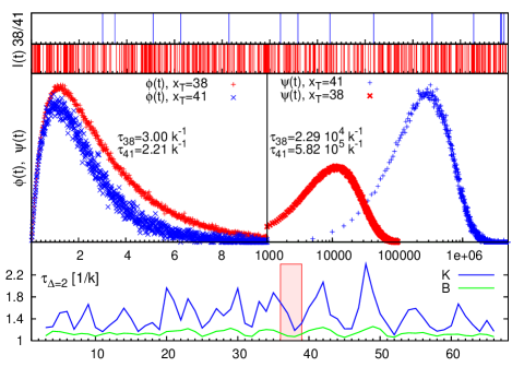
Figure 34: Time series $I(t)$ for the T7 promoter, with $x_{T}=38$, 41. Middle: Waiting time ($\psi(\tau)$) and bubble survival time ($\varphi(\tau)$) densities. Bottom: Mean bubble survival time, $\Delta=2$.

V.7 Interaction of DNA bubbles with selectively single-strand binding proteins

Let us now come back to the destabilising effect of single-stranded DNA binding proteins (SSBs) mentioned in section V.1. In a homopolymer approach, this was studied in a master equation approach in references tobias_pre ; tobias_jpc . The quantity of interest is the joint probability $P(m,n,t)$ to have a bubble consisting of $m$ broken bps, and $n$ SSBs bound to the two arches of the bubble. In addition to the rates $\mathsf{t}^{\pm}$ for bubble increase and decrease, the rates $\mathsf{r}^{\pm}$ for SSB binding and unbinding are necessary to define the breathing dynamics in the presence of SSBs. On the statistical level, the effect of the SSBs becomes coupled to the motion of the zipper forks. Thus, the rate for bubble size decrease is proportional to the probability that no SSB is located right next to the corresponding zipper fork; and the rate for SSB binding is proportional to the probability that there is sufficient unoccupied space on the bubble. Binding is allowed to be asymmetric, and is related to a parking lot problem in the following sense. The number $\lambda$ of bps occupied by a bound SSB is usually (considerably) larger than one. In order to be able to bind in between two already bound SSBs, the distance between these two SSBs must be larger than $\lambda$. The larger $\lambda$ the less efficient the SSB-binding becomes, similar to parking large cars on a parking lot desgined for small vehicles. Apart from the binding size $\lambda$ of the SSBs, two additional physical parameters come into play: the unbinding rate $q$ of the SSBs, and their binding strength $\kappa=c_{0}K^{\mathrm{eq}}$ consisting of the volume concentration $c_{0}$ of SSBs and the equilibrium binding constant $K^{\mathrm{eq}}=v_{0}\exp\left(\beta|E_{\mathrm{SSB}}|\right)$, with the typical SSB volume and binding energy $E_{\mathrm{SSB}}$.

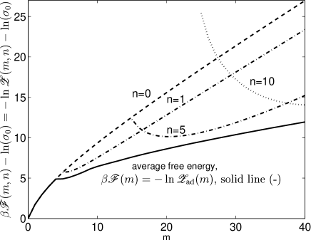
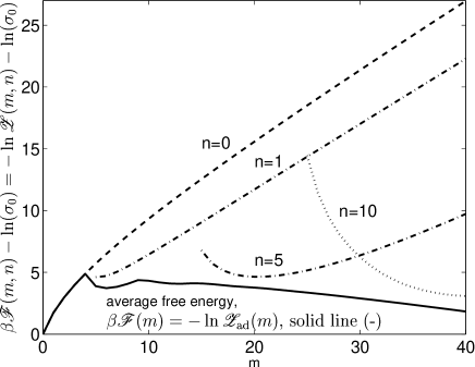
Figure 35: Effective free energy in the limit $\gamma\gg 1$ (—), and ‘free energy’ for various fixed $n$ ($u=0.6$, $M=40$, $c=1.76$, $\lambda=5$). Top: $\kappa=0.5$; bottom: stronger binding, $\kappa=1.5$.

The coupled dynamics of SSB-binding and bubble breathing is discussed in references tobias_pre ; tobias_jpc ; similar effects in end-denaturing DNA was studied in tobias_jpca in detail. Here, we report the behaviour of the effective free energy landscape in the limit of fast SSB-binding in the sense that the dimensionless parameter $\gamma\equiv q/k$ of SSB-unbinding and bubble zipping rates is large, $\gamma\gg 1$. This limit allows one to average out the SSB-dynamics and to calculate an effective free energy, in which the bubble dynamics with the slow variable $m$ runs off. The result for two different binding strengths $\kappa$ is shown in figure 35, along with the free energies corresponding to keeping $n$ fixed. It is distinct that while for lower $\kappa$ the presence of SSBs diminishes the slope of the effective free energy, for larger $\kappa$ the slope actually becomes negative. In the first case, that is, the bubble opening is more likely, but still globally unfavourable. In the latter case, the presence of SSBs indeed leads to full denaturation. One observes distinct finite size effects due to $\lambda>1$: only when the bubble reaches a minimal size $m\geq\lambda$, SSB-binding may occur, a second SSB is allowed to bind to the same arch only once $m\geq 2\lambda$, etc. This effect also produces the nucleation barrier for full denaturation in the lower plot of figure 35. Similar finite size effects were investigated for biopolymer translocation in references tobias_pb ; amlomme . We note that the transition to denaturation could also be achieved by reaching a smaller positive slope of the effective free energy in the presence of SSBs, and additional titration or change of the effective temperature through actual temperature change or mechanical stretching as performed in the experiments reported in references pant ; pant1 ; pant2 .

VI Role of DNA conformations in gene regulation

Our current understanding of gene regulation to large extent is based on the experiments by André Lwoff at Institut Pasteur more than 50 years ago lwoff . Lwoff and his collaborators discovered that while a strain of E.coli, a common intestinal bacterium, divided regularly when undisturbed, an unexpected phenomenon occurred when the strain was exposed to UV light: the bacteria stop growing and after some 90 minutes they burst (lyse), releasing a load of viruses. These viruses then invade new E.coli. Some of the newly infected bacteria immediately lyse again, while the rest divides normally—while carrying the virus in them. This dormant state (lysogeny) of the bacterium can then be driven toward lysis by renewed UV exposure.

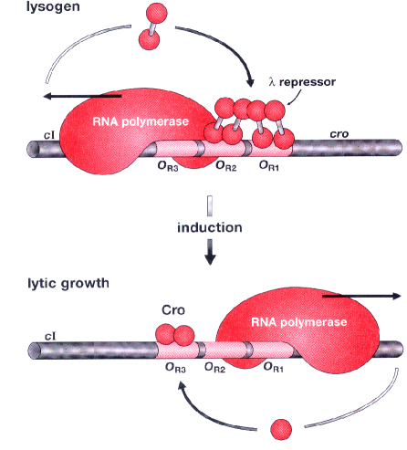
Figure 36: Gene regulation, here the example of the (divergent) bacteriophage $\lambda$ switch after infection of E.coli . Figure from ptashne1 , with permission from M. Ptashne. This figure was modified by the author from the corresponding figure in M. Ptashne, A Genetic Switch: Phage Lambda and Higher Organisms, 2nd edition ©Blackwell Science, Malden, MA and Cell Press, Cambridge, MA, with permission.

The UV exposure-induced transition from lysogeny to lysis occurs as sketched in figure 36. On infection, the bacteriophage $\lambda$ injects its DNA into E.coli . In the lysogenic pathway, the viral DNA is integrated into the host DNA. During lysogeny, repressor dimers bind to certain operator sites on the $\lambda$ part of the DNA, recruiting RNA polymerase to bind to the overlapping promoter region(s) and blocking of the vicinal promoter for the divergent cro gene. RNA polymerase then transcribes the cI gene to the left of the operator, leading to the expression of new repressor molecules. UV light, however, leads to cleavage of the repressor dimers. Now the basal transcription of the gene cro, opposite to the cI gene with respect to the operator region, leads to the expression of the Cro protein. Cro bound to the operator then recruits RNA polymerase to the operator, stabilising the Cro production and blocking cI. Simultaneously, a whole sequence of genes is being expressed, and the virus reproduces itself inside E.coli until lysis occurs. UV light flips the switch from transcription of the gene cI maintaining the dormant lysogenic pathway, inducing lysis that is fostered by transcription of the cro gene ptashne ; ptashne1 .

The activity of a gene can be monitored even on the single genome level, by combining the targeted gene gI with the gene leading to synthesis of GFP, the green fluorescent protein, i.e., when gI is transcribed, then so is the gene for GFP. Occurrence of fluorescence then reports transcription of gI. Connected to questions such as the stability of a genetic pathway is the search process of a specific gene by regulatory proteins, that is, how dynamically the binding protein actually locates the operator on the genome. We address these points in what follows.

VI.1 Physiological background of gene regulation and expression

The $\lambda$ switch from figure 36 is an example of a relatively simple mechanism. Even simpler is the well-studied Lac repressor. There, the lacZ gene is expressed by recruitment through the CAP protein when E.coli is starved of glucose and exposed to lactose. This enables E.coli to digest lactose. In absence of lactose, lacZ is blocked by the rep protein. In general, the expression of a certain gene is just one element in a cascade of simultaneous and/or hierarchical control units, such as in the developmental regulatory network of the sea urchin embryo davidson . The basic physiological background is common to all of them:

Genes are the blueprints of proteins. They control physiological processes but also developmental pathways: from a fertilised egg cell, eventually all cell types (skin, hair, liver, brain, etc cells) of a human body emerge, or a skin cell changes colour on sunlight exposure. A gene is but a stretch of a DNA molecule, typically comprising some 200-1000 bps. Roughly speaking, a gene is on when it is being transcribed by RNA polymerase, otherwise it is off. RNA polymerase binds at the promoter region consisting of some 60 bps close to the beginning of the gene. It then converts the A, T, G, C code of the gene into a complementary messenger RNA (from which, in turn, the protein is produced during translation). The stop of transcription is triggered by a certain sequence at the end of the gene. Depending on specific conditions of the recruitment by regulatory proteins, RNA polymerase binding to the promoter of a certain gene is either blocked (the gene is off), facilitated (high binding affinity of RNA polymerase due to the (simultaneous) presence of certain protein(s)), or basal (in absence of any bound regulatory protein, RNA polymerase can still have a minor affinity to the promoter and then autonomously start transcription). The transcription mechanism is part and parcel of the central dogma of molecular biology summarised in figure 1.

Molecular switches such as the $\lambda$ switch are surprisingly stable against noise, despite the fact that there are only about 100 repressor dimers in the entire bacteria cell reichardt . Thus, apart from external induction, lysis occurs by spontaneous induction due to absence of CI from the operators metzi ; mewo . Such noise-induced errors are estimated to occur once in $10^{7}$ cell generations rozanov ; little2 . The stability of the $\lambda$ switch against noise was analysed in terms of a Wentzell-Freidlin approach aurell and by a simulation analysis aurell1 . The latter confirmed that the currently known molecular mechanisms used in modelling the $\lambda$ switch appear sufficient. While the classical Shea-Ackers model based on a statistical mechanical approach shea is well established and studied numerically arkin , it relies on the knowledge of 13 fundamental Gibbs free binding energies composed to 40 different binding states of regulatory proteins and RNA polymerase at the two promoters of $\lambda$. Simulation of the complete $\lambda$ regulatory system proved the understanding of the mechanisms of the switch arkin . Two more recent studies show that the $\lambda$ switch remains stable even when each of the fundamental Gibbs free energies is varied within its (appreciable) experimental error. Moreover, effects of potential mutations resulting in more significant changes of the binding energies were studied, and it was shown that certain mutations can even be compensated by parallel mutations influencing other binding energies (suppressors) bakk2 ; bakk3 . A typical result is shown in figure 37.

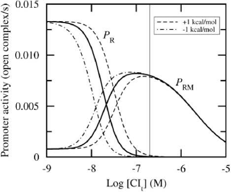
Figure 37: Activity of the two $\lambda$ promoters as function of repressor concentration for vanishing Cro concentration. The full line corresponds to wild type data, whereas the dashed lines correspond to ”mutations”. The thin vertical line corresponds to lysogenic CI concentration. See reference bakk2 for details.

VI.2 Binding proteins: Specific and nonspecific binding modes

Given their very specific function, DNA-binding proteins must recognise a specific (cognate) sequence of nucleotides along the genome. In fact, without opening the double helix, the outside of the DNA can be read by proteins, as the edge of each bp is exposed at the surface. These patterns are unique only in the major groove of the DNA, this being the reason why gene regulatory proteins generally bind to the major groove. Apart from single bp pattern recognition, the protein binding is sensitive to the special surface features of a certain DNA region. This local structure of DNA needs to be complementary to the protein structure. Typical structure patterns (motifs) include helix-turn-helix, zinc fingers, leucine zipper, and helix-loop-helix motifs alberts . In bacteria, typical DNA-binding proteins cover some 20 bps or less. For instance, the lac repressor has a cognate sequence of 21 base pairs, the CAP protein 16, and the $\lambda$ repressor cI 17 bps alberts . Although the interaction with a single nucleotide within such a DNA-protein bond is relatively weak, the sum of all matching nucleotides reaches appreciable values for the overall binding enthalpy, see below. Moreover, regulatory proteins bound simultaneously can significantly enhance the stability of their individual bonds.

A simple model for the binding interaction goes back to the work of Berg and von Hippel bvh ; berg . Accordingly, the binding free energy is comprised of two contributions: (i) the (average) non-specific binding free energy due to electrostatic interaction with the DNA; and (ii) additional binding free energy if the sequence of the binding site is sufficiently close to the best (perfectly matching) sequence. The transition to the non-specific binding is supposed to occur via a conformational change of the regulatory protein from one that allows more hydrogen bond-formation to another that permits closer contact between the positive charges of the binding protein to the negatively charged DNA backbone wbvh . This is supported by more recent structural studies: While in the non-specific binding mode the Lac repressor is bound to DNA in a rather loose and fuzzy way kaladimos , it appears much more ordered in the specific mode. In fact, in the latter the protein induces a bend in the DNA lewis . In case (ii), the additional binding free energy can, to good approximation, be considered independent and additive. reference gerland provides a review of these issues, and derives the following result. Accordingly, to satisfy both the thermodynamic and kinetic constraints of the DNA-binding protein interaction, each additional base mismatch in comparison to the best sequence amounts to the loss of roughly 2 $k_{B}T$, and the optimal value for the transition between best specific binding to the cognate site and non-specific binding is shown to be some 16 $k_{B}T$ below the energy of the best binding. This value is quite close to the $\approx 14$ $k_{B}T$ found for the difference between specific and nonspecific binding in bakk ; bakk1 .

The fact that regulatory proteins bind with varying affinity is an important ingredient in gene regulation: Not all promoters should have the same activity, because some proteins are required by the cell at much higher levels than others. Thus, one given regulatory protein, that controls the recruitment to the promoters of several genes, can act with different strength depending on the degree of matching with the local sequence.

Non-specific binding can become quite appreciable. It was discovered in reference kao that in the case of the Lac repressor less than 10% of the proteins were unbound. In a more recent study using in vivo data of the $\lambda$ switch, it was found that in a lysogen nearly 90% of the repressor protein cI is non-specifically bound. This implies that only 10-20 free cI dimers exist in the E.coli cell at any time, pointing at the important role of non-specific binding in the search process of the cognate site addressed in the following subsection. Under different conditions, both cI and Cro are always non-specifically bound by more than 50%. The corresponding non-specific binding energies were estimated as 7 $k_{B}T$ bakk ; bakk1 .

We note that in contrast to regulatory proteins, restriction enzymes have an approximate all-or-nothing matching condition: If a defined sequence matches the restriction enzyme, it will cut, otherwise not. Even a single mismatch reduces the action of the restriction enzyme by orders of magnitude. This distinction from regulatory protein makes sense as restriction enzymes are survival mechanisms and should not just cut the cell’s own DNA stormo . This does not mean that restriction enzymes do not bind non-specifically—in fact, this is an important ingredient of their search process in total analogy to regulatory proteins. However, their sole active role occurs on complete matching.

VI.3 The search process for the specific target sequence

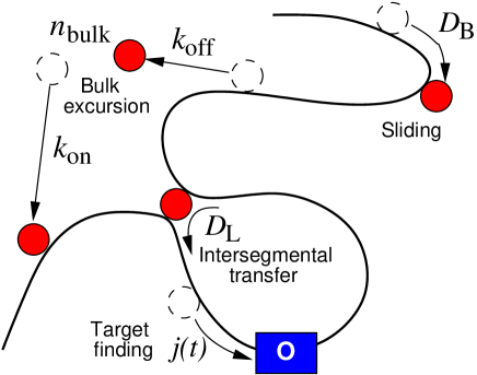
Figure 38: Schematic of the search mechanisms in equation (52).

To find their specific (cognate) binding site along the genome, DNA-binding proteins such as restriction enzymes or transcription factors have to search megabases along the DNA molecule. The high accuracy of gene expression control by binding proteins such as in the $\lambda$-switch requires a fast search and recognition of the target sequence by the proteins. A simple 3-dimensional (3D) search of the target sequence by the proteins is not sufficient to explain experimentally measured target search rates. It has been suggested relatively early adam ; eigen that additional search mechanisms such as 1D sliding along the genome are needed to account for the actual efficiency of the search process. In their pioneering work, Berg, von Hippel and coworkers established a statistical model for target search comprising the four fundamental steps, as shown in figure 38: (i) 3D macrohops during which the protein fully detaches from the genome until after a volume excursion it rebinds to the DNA (as a good approximation, the landing site on the DNA after a macrohop can be assumed to be equidistributed and uncorrelated); (ii) microhops during which the protein detaches from the DNA but always stays very close to it (i.e., the microhop takes place within a cylinder whose radius corresponds to the escape distance of the protein from the DNA, see berg ); (iii) 1D sliding along the genome (while preserving a certain bonding to the DNA due to nonspecific binding); and (iv) intersegmental jumps. The latter are mediated by DNA-loops bringing two chemically remote segments of the DNA close in Euclidean space, see, for instance, hame_looping and references therein. A protein like Lac repressor, which can establish bonds to two different stretches of dsDNA simultaneously, can then jump from one to the neighbouring segment. This process might lead to a paradoxical diffusion behaviour paradox ; dirk . However, if the conformational changes in the DNA are not too slow, both the bulk mediated macrohops and the intersegmental transfer lead to fast mixing of the enzymes’ positions along the chain (as it was shown for the related problem in JLum ), and on the mean-field level can be described by a desorption followed by the absorption at a random place.

Recently, there has been renewed interest in the targeting problem, both theoretically (see, for instance, gerland ; slutsky ; marko2 ; coppey ) and experimentally (e.g., grillo ; record ), including single molecule studies shima ; pant1 ; pant2 . Despite the extensive knowledge of specific binding rates and both specific and non-specific binding free energies, the precise relative contributions of the different search mechanisms (and, to some extent, also the stringent criteria to define these four elementary interactions) are not fully resolved. Moreover, it has been suggested that under tight(er) binding conditions, the sliding of the protein becomes subdiffusive due to the local structure landscape of a heteropolymer DNA slutsky1 . This complication, however, is expected to be relaxed in a more loosely bound search mode of the searching protein slutsky . We here adopt the latter view of normal diffusion, which is corroborated by the experimental study in the next subsection.

VI.4 A unique situation: Pure one-dimensional search of SSB mutants

In previous studies, the 1D sliding problem had always been considered as a problem of 3D diffusion which is enhanced by 1D diffusion. Thus, workers such as Berg, Winter, and von Hippel berg assumed that proteins nonspecifically bound would on average unbind before finding their specific binding sites. This results in an enhancement of specific binding rates that is proportional to the 1D sliding rate, but the overall specific binding rate depends linearly on protein concentration. These studies neglect the possibility that the protein finds its specific site before unbinding. Given the experimental conditions under which transcription factor binding has been previously studied, this approximation is appropriate. However, as demonstrated in igor_prot , this mechanism, in which the unbinding rate is much lower than the specific binding rate, occurs for the 1D search of DNA by the single-stranded DNA binding protein T4 gene 32 protein (gp32). This fast 1D search rate is essential for gp32 to be able to quickly find specific locations on DNA molecules that are undergoing replication, and which have large sections of single-stranded DNA exposed for gp32 binding. The resulting nonlinear concentration dependence of gp32 binding will likely have significant effects on gp32’s ability to find its replication sites as well as its ability to recruit other proteins during replication. If these nonlinear effects also occur for TFs, this characteristic will strongly affect regulatory processes governed by protein binding.

Figure 39: Dimensional binding rate $k_{a}$ in 1/s as function of protein concentration $C$ in M, for parameters corresponding to 100 mM salt. The fitted 1D diffusion constant for sliding along the dsDNA is $D_{\mathrm{1d}}=3.3\cdot 10^{-9}\mathrm{cm}^{2}/\mathrm{sec}$, located nicely within the experimental value $10^{-8}\ldots 10^{-9}\mathrm{cm}^{2}/\mathrm{sec}$ pant .

Results from the single DNA overstretching experiment are shown in figure 39 along with the results from the theoretical and simulations analysis from references igor_prot . The scaling of search rate as function of concentration is described by the relation

$$k_{a}=D_{\mathrm{1d}}n_{0}^{2}$$ (51)

obtained for the pure 1D search of random walkers of line density $n_{0}^{2}$ searching along the DNA. For low concentrations, the McGhee and von Hippel isotherm mcghee predicts a linear relation between $n_{0}$ and the volume concentration $C$; thus, $k_{a}\propto C^{2}$. The experimental evidence for the purely linear search process, as shown in figure 39 for 100 mM salt, was found for a large range of salt concentrations, see references igor_prot ; pant2 for details. The case of high line density of proteins was discussed in igor_finite .

VI.5 Lévy flights and target search

We now address the general search process with interchange of 1D and 3D diffusion, and intersegmental jumps. To this end, we first quickly review the definition of Lévy flights klafternature ; physicstoday ; report ; report1 ; coffey .

Lévy flights (LFs) are random walks whose jump lengths $x$ are distributed like $\lambda(x)\simeq|x|^{-1-\alpha}$ with exponent $0<\alpha<2$ hughes . Their probability density to be at position $x$ at time $t$ has the characteristic function $P(q,t)\equiv\int_{-\infty}^{\infty}e^{iqx}P(x,t)dx=\exp\left(-D_{\mathrm{L}}|q|^{\alpha}t\right)$, a consequence of the generalised central limit theorem levy ; gnedenko ; in that sense, LFs are a natural extension of normal Gaussian diffusion ($\alpha=2$). LFs occur in a wide range of systems report ; in particular, they represent an optimal search mechanism in contrast to locally oversampling Gaussian search stanley . Dynamically, LFs can be described by a space-fractional diffusion equation $\partial P/\partial t=D_{\mathrm{L}}\partial^{\alpha}P(x,t)/\partial|x|^{\alpha}$, a convenient basis to introduce additional terms, as shown below. $D_{\mathrm{L}}$ is a diffusion constant of dimension $\mathrm{cm}^{\alpha}/\mathrm{sec}$, and the fractional derivative is defined via its Fourier transform, $\mathscr{F}\{\partial^{\alpha}P(x,t)/\partial|x|^{\alpha}\}=-|q|^{\alpha}P(q,t)$ report ; report1 ; coffey . LFs exhibit superdiffusion in the sense that $\langle|x|^{\zeta}\rangle^{2/\zeta}\simeq D_{\mathrm{L}}t^{2/\alpha}$ ($0<\zeta<\alpha$) report , spreading faster than the linearly growing mean squared displacement of standard diffusion ($\alpha=2$). A prime example of an LF is linear particle diffusion to next neighbour sites on a fast folding (‘annealed’) polymer that permits intersegmental jumps at chain contact points (see figure 38) caused by polymer looping paradox ; dirk . In fact, the contour length $|x|$ stored in a loop between such contact points is distributed in 3D like $\lambda(x)\simeq|x|^{-1-\alpha}$, where $\alpha=1/2$ for Gaussian chains ($\theta$ solvent), and $\alpha\approx 1.2$ for self-avoiding walk chains (good solvent) duplantier .

In our description of the target search process, we use the density per length $n(x,t)$ of proteins on the DNA as the relevant dynamical quantity ($x$ is the distance along the DNA contour). Apart from intersegmental transfer, we include 1D sliding along the DNA with diffusion constant $D_{\mathrm{B}}$, protein dissociation with rate $k_{\mathrm{off}}$ and (re)adsorbtion with rate $k_{\mathrm{on}}$ from a bath of proteins of concentration $n_{\mathrm{bulk}}$. The dynamics of $n(x,t)$ is thus governed by the equation michael

$$\frac{\partial}{\partial t}n(x,t)= \left(D_{\rm B}\frac{\partial^{2}}{\partial x^{2}}+D_{\rm L}\frac{\partial^{\alpha}}{\partial|x|^{\alpha}}-k_{\rm off}\right)n(x,t)$$ (52)

$$+k_{\rm on}n_{\rm bulk}-j(t)\delta(x).$$

Here, $j(t)$ is the flux into the target located at $x=0$. We determine the flux $j(t)$ by assuming that the target is perfectly absorbing: $n(0,t)=0$ chechkin_bvp . Be initially the system at equilibrium, except that the target is unoccupied; then, the initial protein density is $n_{0}=n(x,0)=k_{\rm on}n_{\rm bulk}/k_{\rm off}$. The total number of particles that have arrived at the target up to time $t$ is $J(t)=\int_{0}^{t}dt^{\prime}\;j(t^{\prime})$. We derive explicit analytic expressions for $J(t)$ in different limiting regimes, and study the general case numerically. We use $J(t)$ to obtain the mean first arrival time $T$ to the target; in particular, to find the value of $k_{\rm off}$ that minimises $T$.

Figure 40: Optimal choice of off rate $k_{\rm off}$ as function of the LF diffusion constant, from numerical evaluation of the model in reference michael . The circle on the abscissa marks where $k_{\rm off}^{\rm opt}$ becomes 0 in the case $\alpha<1/2$.

The various regimes of target search embodied in equation (52) are discussed in detail in references michael ; michael_long . The main result for the efficiency of the related search process is summarised in figure 40, i.e., which protein unbinding rate $k_{\mathrm{off}}$ optimises the mean search time $T$. Three regimes can be distinguished:

(i) Without Lévy flights, we obtain $k_{\rm off}^{\rm opt}=k_{\rm on}^{\prime}$: the proteins should spend equal amounts of time in bulk and on the DNA. This corresponds to the result obtained for single protein searching on a long DNA slutsky ; coppey .

(ii) For $\alpha>1$, i.e., when DNA is in the self-avoiding regime, we find

$$k_{\rm off}^{\rm opt}\sim(\alpha-1)k_{\rm on}^{\prime}:$$ (53)

The optimal off rate shrinks linearly with decreasing $\alpha$.

(iii) For $\alpha<1$, i.e., when DNA leaves the self-avoiding phase (e.g., by lowering the temperature or introducing attractive interactions) the value of $k_{\rm off}^{\rm opt}$ approaches zero as the frequency of intersegmental jumps ($\propto D_{L}$) increases: The Lévy flight mechanism becomes so efficient that bulk excursions become irrelevant. At $\alpha=1/2$, the case of the ideal Gaussian chain, we observe a qualitative change: When $\alpha<1/2$, the rate $k_{\rm off}^{\rm opt}$ reaches zero for finite values of the rate for intersegmental jumps. Note that when $\alpha<1$, the spread of the Lévy flight ($\simeq t^{1/\alpha}$) grows faster than the number of sites visited ($\simeq t$), rendering the mixing effect of bulk excursions insignificant. A scaling argument to understand the crossover at $\alpha=1/2$ relates the probability density of first arrival with the width ($\simeq t^{1/\alpha}$) of the Green’s function of a Lévy flight $p_{\mathrm{fa}}\simeq t^{-1/\alpha}$. We see that the associated mean arrival time becomes finite for $0<\alpha<1/2$, even for the infinite chain limit considered here.

We remark that this model is valid for an annealed DNA only. This means that the chain can equilibrate (at least, locally) on the typical time scale between intersegmental jumps. Even though real DNA in solution might not be fully annealed, features of this analysis will reflect on the target search. A more detailed study of different regimes of DNA is under way.

VI.6 Viruses—extreme nanomechanics

Viruses have played an important role in the discovery of the mechanisms underlying gene regulation, see, for instance, reference lwoff . From a nanoscience perspective, viruses are of interest on their own part. During the assembly of many viruses, the viral DNA of several $\mu$m length is packaged into the capsid, the protein container making up most of the virus, by a motor protein. This motor packages the DNA by exerting forces of up to 60 pN or more, causing pressures building up in the capsid of the order of 6 MPa smith ; zandi . The size of the capsid spans few tens of $\mu$m, and is therefore comparable to the persistence length of DNA feiss ; morita ; smith ; hud1 ; hud . Therefore, fluctuation-based undulations are suppressed, and the chain can be approximately thought of as being wound up helically like thread on a bobbin, or like a ball of yarn. Ultimately, a relatively highly ordered 3D configuration of the DNA inside the capsid is achieved, which under certain conditions may even lead to local crystallisation of the DNA feiss ; morita ; pack ; hud ; kindt ; kondev1 ; ali . It is generally argued that this ordered arrangement helps to avoid the creation of entanglements or even knots of the wound-up DNA, thus enabling easy ejection, i.e., release of the DNA once the phage docks to a new host cell; this ejection is not assisted by the packaging motor, but it can be facilitated by host cellular DNA polymerase, which starts to transcribe the DNA and thereby pulls it out of the capsid alberts ; snustad ; kindt ; arsuaga . Details on the packaging energetics can be found in reference pack , and the works cited therein. Model calculations for the entropy loss, binding and twist energy, and electrostatic forces that need to be overcome on packaging reveal, that at higher packaging ratios the packaging force almost exclusively comes from the electrostatic repulsion.

VII Functional molecules and nanosensing

Complex molecules can be endowed with the distinct feature that they contain subunits which are linked to each other mechanically rather than chemically schill . The investigation of the structure and properties of such interlocked topological molecules is subject of the growing field of chemical topology frisch ; while speculations about the possibility of catenanes (Olympic rings) date back to the early 20th century lectures of Willstätter, the actual synthesis of catenanes and rotaxanes succeeded in 1958 schill . Modern organic chemistry has seen the development of refined synthesis methods to generate topological molecules.

VII.1 Functional molecules

In parallel to the miniaturisation in electronics bishop and the possibility of manipulating single (bio)molecules strick1 , supramolecular chemistry which makes use of chemical topology properties is coming of age lehn ; dietrich . Thus, rotaxane-type molecules are believed to be the building blocks for certain nanoscale machines and motors blanco , so-called hermaphrodite molecules have been shown to perform linear relative motion (“contraction and stretching”) jimenez , and pirouetting molecules have been synthesised raehm . Moreover, topological molecules are thought to become components for molecular electronics switching devices in memory and computing applications pease ; lehn1 . These molecular machines are usually of lower molecular weight, and their behaviour is essentially energy-dominated in the sense that their conformations and dynamical properties are governed by external and thermal activation in an energy landscape. The understanding of the physical properties and the theoretical modelling of such designer molecules and their natural biological counterparts has increasingly gained momentum, and the stage is already set for the next generation of applications bishop ; strick1 ; lehn ; dietrich ; blanco ; jimenez ; raehm ; pease ; lehn1 ; montemagno ; soong ; yurke ; metz ; motors ; frey .

In reference hame_cpl we introduced some basic concepts for functional molecules whose driving force is entropic rather than energetic, see also the more recent publications in chemistry journals functional ; functional1 . Entropy-functional molecules will be of higher molecular weight (hundred monomers or above) in order to provide sufficient degrees of freedom such that entropic effects can determine the behaviour of the molecule. The potential for such entropy-driven functional molecules can be anticipated from the classical Gibbs Free energy

$$\mathscr{F}=U-TS\,;$$ (54)

in functional molecules, $\mathscr{F}$ is minimised mainly by variation of the internal energy $U$ representing the shape of the energy landscape of the functional unit. New types of molecules were proposed for which $\mathscr{F}$ is minimised by variations of the entropy $S$, while the energies and chemical bondings are left unchanged hame_cpl . The entropy-functional units of such molecules can be specifically controlled by external parameters like temperature, light flashes, or other electromagnetic fields lehn ; dietrich . We note that DNA is already being studied as a macromolecular prototype building block for molecular machines yurke .

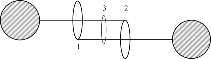
Figure 41: Molecular muscle consisting of two interlocked rings 1 and 2 with attached rod-like molecules. Within this structure, sliding rings, 3, can be placed, which, if activated, tend to contract the muscle by entropic forces.

A typical example is the molecule shown in figure 41. According to the arrangement of the sliding rings 1 and 2, this compound exhibits the unique feature of a molecule that it can slide laterally. Suggested as precursors of molecular muscles jimenez , this compound could be propelled with internal entropy-motors, which entropically adjust the elongation of the muscle. In the configuration shown in figure 41, the sliding ring 3 creates, if activated, an entropic force which tends to contract the “muscle”; at $T=300\,{\mbox{K}}$ and on a typical scale $x=10\,\mbox{nm}$, the entropic force $k_{B}T/x$ is of the order of pN, and thus comparable to the force created in biological muscle cells gittes . Molecular muscles of such a make can be viewed as the nano-counterpart of macroscopic muscle models proposed by de Gennes degennesm , in which the contraction is based on the entropy difference between the isotropic and nematic phases in liquid crystalline elastomer films thomsen .

Similarly, one might speculate whether the DNA helix-coil transition poland in multiplication setups could be facilitated in the presence of pre-ring molecules which in vitro attach to an opened loop of the double strand and close, creating an entropy pressure which tends to open up the vicinal parts of the DNA which are still in the helix state. Finally, considering molecular motors, it would be interesting to design an externally controllable, purely entropy-driven rotating nanomotor.

Numerous additional nanoapplications of biopolymers appear in current literature. An interesting example is the nanomotor created by a DNA ring in a periodically driven external field, for instance, a focused light beam inducing localised temperature variations kulic_schiessel ; kulic_schiessel_jpc . The speeds possibly attained by such a device are of the order of those reached by biological organisms. Such a nanorotor could be used to stir smallest volumes in higher viscous environments.

VII.2 Nanosensing

The advances in minituarization of reactors and devices also brings along the need of probes, by which smallest volumes can be tested. For instance, microarrays used in genomics require sensors to detect the presence of certain proteins (often at small concentrations) in a microdish, without disturbing the environment in the small volume too much. Similarly, single molecule experiments require specific local detection possibilities.

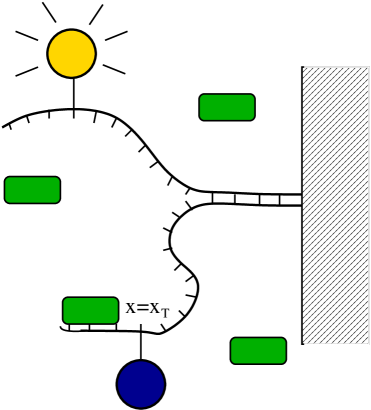
Figure 42: Molecular beacon based on local DNA denaturation. The green blobs may represent single-stranded DNA binding proteins, or more specifically binding proteins binding or other molecule to a custom designed DNA sequence along the denaturation fork. Bound proteins stabilize the denatured fork and change the spectrum of the beacon.

A fine example for a potential nanosensore is the blinking behaviour of a fluorophore-quencher pair mounted on the denaturation wedge as shown in figure 42. This setup, similar to the ones described in references altan ; oleg1 works as follows. As long as the dsDNA is intact, fluorophore and quencher are in close proximity. Once they come apart from one another when the denaturation wedge opens up, the incident laser light causes fluorescence of the dye. The on/off blinking of this ”molecular beacon” can be monitored in the focus of a confocal microscope, or, depending on the intensity of the emitted light, by a digital camera. The blinking renders immediate information about the state of the bp, that is tagged by the dye-quencher pair. Fluorescence, that is, indicates that the bp is currently broken. It is therefore advantageous to define the random variable $I(t)$ with the property

$$I(t)=\left\{\begin{array}[]{ll}0&\mbox{if base-pair at $x=x_{T}$ is closed}\\ 1&\mbox{if base-pair at $x=x_{T}$ is open}\end{array}\right.,$$ (55)

and in experiments one typically measures the corresponding blinking autocorrelation function

$$A(t)=\langle I(t)I(0)\rangle-\langle I\rangle_{\mathrm{eq}^{2}},$$ (56)

where $\langle I\rangle_{\mathrm{eq}}$ is the (ensemble) equilibrium value, or its spectral decomposition

$$A(t)=\int_{0}^{\infty}f(\tau)\exp\left(-\frac{t}{\tau}\right)d\tau,$$ (57)

where

$$f(\tau)=\sum_{p\neq 0}T_{p}^{2}\delta\left(\tau-\tau_{p}\right).$$ (58)

is called the relaxation time spectrum.

Figure 43 shows an example for the achievable sensitivity of such nanobeacons, in an example where the denaturation wedge is in solution together with a certain concentration (proportional to $\kappa$, compare Sec. IVG) of selectively single-stranded DNA binding proteins, as discussed previously. It is distinct how both measurable signals, $A(t)$ and $f(\tau)$ change with varying SSB-concentration.

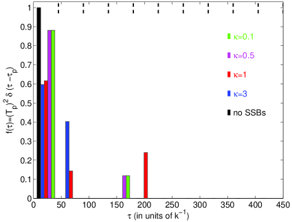
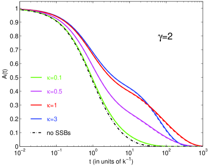
Figure 43: Spectral response of the denaturation beacon in the presence of single-stranded DNA binding proteins. Top: Relaxation time spectrum, bottom: blinking autocorrelation function.

VIII Summary

Biopolymers such as DNA, RNA, and proteins are indispensable for their specificity and robustness in all forms of life. Given their detailed physical properties such as DNA’s persistence length of some 50nm or its local denaturation in nano-bubbles already at room temperature, and biochemically relevant interfaces such as 10-20 bps, they deeply stretch into the nanoscience domain. This statement is twofold in the following sense. Firstly, nanotechniques such as atomic force microscopes become important tools to manipulate and probe biomolecules and their interaction even on the single molecule level. Secondly, biomolecules are entering the stage as nanotools such as nanosensors, functional molecules, or highly sensitive force transducers.

The possibility to perform controlled experiments on biomolecules, for instance, to measure the force-extension curves of single biopolymers, also opens up novel possibilities to test new physical theories. The foremost examples may be the exploration of persistence lengths and other polymer physics properties, and the statistical mechanical concepts relevant for small system sizes. The latter are known under the keyword of the Jarzynski relation connecting the non-equilibrium work performed on a physical system with the difference in the thermodynamic (i.e., equilibrium) potential between initial and final states jarzinsky ; udo . However, there exist by now several similar theories addressing different physical quantities, such as the concept of entropy production along a single particle trajectory udo1 .

This review summaries fundamental physical properties of DNA, and their relevance for both biological processes and technological applications. The extensive list of references will be useful for further studies on specific topics covered herein. We are confident that the role of biomolecules in technology, not at least for biomedical applications, will experience a dramatic increase during the coming years and will enable us to extend current physical understanding of fundamental processes.

Biographical notes

Ralf Metzler received his doctoral degree in physics from the University of Ulm, FRG. He then went to Tel Aviv University as Humboldt Feodor Lynen fellow and later as Minerva Amos de Shalit fellow, to work with Joseph Klafter. As DFG Emmy Noether fellow, after a period as visiting scientist at the University of Illinois at Urbana-Champaign with Peter Wolynes, Ralf moved to the Massachusetts Institute of

Technology (MIT) in Cambridge, MA, where he worked with Mehran Kardar. In 2002 Ralf was appointed Assistant Professor at the Nordic Institute for Theoretical Physics (NORDITA) in Copenhagen, Denmark. In summer 2006, Ralf assumed his post as Associate Professor and Canada Research Chair in Biological Physics at the University of Ottawa, Canada. Ralf works extensively on biological physics problems and anomalous stochastic processes. These include DNA physics such as DNA denaturation, DNA topology and the role of DNA conformations in gene regulation, as well as anomalous diffusion in biological systems. The latter questions are connected with Lévy statistics leading to, respectively, subdiffusion or Lévy flights. In his spare time, Ralf enjoys the company of his daughter and wife, he listens to classical music and is a keen reader of murder mysteries. In Canada, Ralf is looking forward to nature walks, cross-country skiing and ice-skating.

Tobias Ambjörnsson received his PhD from Chalmers and Gothenburg University, where he worked on the electromagnetic response of matter. In 2003 he became a NORDITA postdoctoral fellow, working with Ralf Metzler on the modelling of single biomolecule problems such as DNA breathing and biopolymer translocation through nanopores. Tobias re-

recently received a prestigious fellowship from the Wallenberg foundation, allowing him to join the group of Robert Silbey at MIT in autumn 2006, to pursue studies on nanosensors. Tobias enjoys listening to pop music, travelling, and spending time with friends.

Andreas Hanke received his doctoral degree in physics from the University of Wuppertal in Germany, FRG. He then went to the Massachusetts Institute of Technology (MIT) for his postdoctoral studies with Mehran Kardar. After a period as visiting scientist with Michael Schick at the University of Washington, Seattle, he moved to a postdoc-

toral position in John Cardy’s group at the University of Oxford, UK, followed by postdocs with Udo Seifert in Stuttgart, FRG, and again with John Cardy in Oxford. In 2004 Andreas became Assistant Professor of Physics at the University of Texas at Brownsville. He is also Adjunct Assistant Professor at the Department of Physics at The University of Texas at Dallas and a member of the Institute of Biomedical Sciences and Technology at UT Dallas. In addition, his research includes summer appointments at the UT Dallas NanoTech Institute. Andreas has worked in the fields of mesoscopic quantum systems, soft condensed matter physics, and biological physics. Currently he is building up a theory division in Molecular Biophysics and Nanoscience at the University of Texas at Brownsville. In his spare time, Andreas enjoys latin and salsa music and dancing, all kinds of outdoor activities, and excursions to Mexico.

Yongli Zhang is a postdoctoral fellow of the Jane Coffin Childs Memorial Fund for Medical Research in Carlos Bustamante’s group at University of California at Berkeley. He received his Ph.D. in Molecular Biophysics and Biochem-

Biochemistry from Yale University in 2003, under supervision of Donald Crothers. In December 2006, he will move to the Department of Physiology and Biophysics at Albert Einstein College of Medicine as an assistant professor. Yongli has been doing both experimental and theoretical research in DNA mechanics, chromatin dynamics, and mechanism of chromatin remodeling. His lab will mainly use single-molecule techniques, such as optical tweezers and atomic force microscopy, to study mechanism of molecular motors and dynamics of macromolecular assemblies.

Stephen Levene is Associate Professor of Molecular and Cell Biology at The University of Texas at Dallas. Dr. Levene received his Ph.D. in Chemistry from Yale University in 1985 and was an American Cancer Society postdoctoral fellow with Bruno Zimm at University of California,

San Diego until 1989. He then spent one year as a staff scientist at the Human Genome Center at Lawrence Berkeley Laboratory and was a Program in Mathematics and Molecular Biology Fellow at University of California, Berkeley in Nicholas Cozzarelli’s laboratory. Dr. Levene’s research interests are in the area of nucleic-acid structure and flexibility, mechanisms of DNA recombination, the structural organization of human telomeres, and applications of these areas to biotechnology. He leads the focus group in Molecular Diagnostics and Bioimaging in the UT-Dallas Institute of Biomedical Sciences and Technology, is recipient of an Obermann Interdisciplinary Research Fellowship, a member of the Biophysical Society, and has served on several NIH study sections. In addition to scientific pursuits, Dr. Levene is an avid snow skier and cyclist, having previously competed in both disciplines.

A polymer primer.

In this section, we introduce some basic concepts from polymer physics. Starting from the random walk model, we define the fundamental measures of a polymer chain, before introducing excluded volume. For more details, we refer to the monographs degennes ; doi ; grosberg ; flory .

The simplest polymer model is due to Orr orr . It models the polymer chain a a random walk on a periodic lattice with lattice spacing $a$. Then, each monomer of index $i$ is characterised by a position vector $\mathbf{R}_{i}$ with $i=0,1,\ldots,N$. The distance between monomers $i$ and $i+1$ is called $\mathbf{a}_{i+1}=\mathbf{R}_{i+1}-\mathbf{R}_{i}$. Consequently, the end-to-end vector of the polymer is

$$\mathbf{r}=\sum_{i}\mathbf{a}_{i}.$$ (59)

Different $\mathbf{a}_{i}$ have completely independent orientations, such that we immediately obtain the average ($\langle\cdot\rangle$ over different configurations) squared end-to-end distance

$$\mathbf{R}_{0}^{2}=\langle\mathbf{r}^{2}\rangle=\sum_{i,j}\langle\mathbf{a}_{i}\cdot\mathbf{a}_{j}\rangle=\sum_{i}\langle\mathbf{a}_{i}^{2}\rangle=Na^{2}.$$ (60)

$R_{0}\simeq N^{1/2}a$ is a measure for the size of the random walk. An alternative measure of the size of a polymer chain is provided by its radius of gyration $R_{g}$, which may be measured by light scattering experiments. It is defined by

$$R_{g}^{2}=\frac{1}{1+N}\sum_{i=0}^{N}\langle\left(\mathbf{R}_{i}-\mathbf{R}_{G}\right)^{2}\rangle,$$ (61)

and measures the average squared distance to the centre of gravity,

$$\mathbf{R}_{G}=\frac{1}{1+N}\sum_{i=0}^{N}\mathbf{R}_{i}.$$ (62)

Expression (61) can be rewritten as

$$R_{g}^{2}=(1+N)^{-2}\sum_{i=0}^{N-1}\sum_{j=i+1}^{N}\langle\left(\mathbf{R}_{i}-\mathbf{R}_{j}\right)^{2}\rangle.$$ (63)

With $\mathbf{R}_{j}-\mathbf{R}_{i}=\sum_{n=i+1}^{j}\mathbf{a}_{n}$, one can easily show that $R_{g}^{2}=a^{2}N(N+2)/[6(N+1)]$. For large $N$, that is, $R_{g}\simeq\frac{a^{2}}{6}N$, and therefore:

$$R_{g}\sim R_{0}\sim aN^{1/2}.$$ (64)

On a cubic lattice in $d$ dimensions, each step can go in $2d$ directions, and for a general lattice, each vector $\mathbf{a}_{i}$ will have $\mu$ possible directions. The number of distinct walks with $N$ steps is therefore $\mu^{N}$. Denote $\mathfrak{N}_{N}(\mathbf{r})$ the number of distinct walks with end-to-end vector $\mathbf{r}$, the probability density function for a given $\mathbf{r}$ is

$$p(\mathbf{r})=\frac{\mathfrak{N}_{N}(\mathbf{r})}{\sum_{\mathbf{r}}\mathfrak{N}_{N}(\mathbf{r})}.$$ (65)

For large $N$, due to the independence of individual $\mathbf{a}_{i}$, this probability density function will acquire a Gaussian shape,

$$p(\mathbf{r})=\left(\frac{d}{2\pi Na^{2}}\right)^{d/2}\exp\left(-\frac{dr^{2}}{2Na^{2}}\right),$$ (66)

where the normalisation is such that $\langle\mathbf{r}^{2}\rangle=Na^{2}$. From this expression, we can deduce that the number of degrees of freedom of a closed random walk chain is proportional to $N^{-d/2}$, the entropy loss suffered by a chain subject to the constraint $\mathbf{r}=0$. On a general lattice,

$$\omega\simeq\mu^{N}N^{-d/2}$$ (67)

with the connectivity constant $\mu$, a measure for in how many different directions the next bond vector can point ($\mu=2d$ in a cubic lattice). At fixed end-to-end distance, the entropy of the random walk becomes $S(\mathbf{r})=S_{0}-dr^{2}/(2Na^{2})$ where $S_{0}$ absorbs all constants. For the free energy $\mathscr{F}(\mathbf{r})=E-k_{B}TS(\mathbf{r})$ we therefore obtain

$$\mathscr{F}(\mathbf{r})=\mathscr{F}_{0}+\frac{dk_{B}Tr^{2}}{2R_{0}^{2}},$$ (68)

i.e., the random walk likes to coil, the restoring force $-\nabla\mathscr{F}(\mathbf{r})$ being linear in $\mathbf{r}$. This is often called the entropic spring character of a Gaussian polymer. Note that the ‘spring constant’ increases with temperature (‘entropy elasticity’).

In this random walk model of a polymer chain, it is straightforward to define the persistence length of the chain. By this we mean that successive vectors $\mathbf{a}_{i}$ are not independent, but tend to be parallel. Over long distance, this correlation is lost, and the chain behaves like a random walk. Due to the quantum chemistry of the monomers, an adjacent pair of vectors $\mathbf{a}_{i},\mathbf{a}_{i+1}$ includes preferred angles, for carbon chains leading to the trans/gauche configurations. This feature is captured schematically in the freely rotating chain as depicted in figure 44.

Figure 44: Freely jointed chain, in which successive bond vectors include an angle $\theta$.

Following doi , we can obtain the correlation $\langle\mathbf{a}_{n}\cdot\mathbf{a}_{m}\rangle$ as follows. If we fix all vectors $\mathbf{a}_{m},\ldots,\mathbf{a}_{n-1}$, then the average $\langle\mathbf{a}_{n}\rangle_{\mathbf{a}_{m},\mathbf{a}_{m+1},\ldots,\mathbf{a}_{n-1}\mbox{ fixed}}=\mathbf{a}_{n-1}\cos\theta$. Multiplication by $\mathbf{a}_{m}$ produces

$$\langle\mathbf{a}_{m}\cdot\mathbf{a}_{n}\rangle_{\mathbf{a}_{m},\ldots,\mathbf{a}_{n-1}\mbox{ fixed}}=\mathbf{a}_{m}\cdot\mathbf{a}_{n-1}\cos\theta.$$ (69)

Averaging over the $\mathbf{a}_{m},\ldots,\mathbf{a}_{n-1}$ leads to the recursion relation $\langle\mathbf{a}_{m}\cdot\mathbf{a}_{n}\rangle=\langle\mathbf{a}_{m}\cdot\mathbf{a}_{n-1}\rangle\cos\theta$. With the initial condition $\langle\mathbf{a}^{2}\rangle=a^{2}$, we find

$$\langle\mathbf{a}_{m}\cdot\mathbf{a}_{n}\rangle=a^{2}\cos^{|n-m|}\theta.$$ (70)

Thus, if $\theta=0$, we obtain a rigid rod behaviour, while for $\theta\neq 0$, there occurs an exponential decay of the correlation between any two bond vectors $\mathbf{a}_{n}$ and $\mathbf{a}_{m}$. This defines a length scale

$$\ell_{p}\equiv\frac{a}{\log\cos\theta},$$ (71)

the ‘persistence length’ of the chain. It diverges for $\theta\to 0$, while for $\theta=90^{\circ}$, it vanishes, corresponding to the random walk model discusses above (‘freely jointed chain’). As

$$\sum_{k=-\infty}^{\infty}\langle\mathbf{a}_{n+k}\cdot\mathbf{a}_{n}\rangle=a^{2}\left(1+2\sum_{k=1}^{\infty}\cos^{k}\theta\right)=a^{2}\frac{1+\cos\theta}{1-\cos\theta},$$ (72)

we find $R_{0}^{2}=a^{2}N(1+\cos\theta)/(1-\cos\theta)$, i.e., statistically, the freely jointed chain behaves the same as the random walk chain, but with a rescaled monomer length. The statistical unit in a polymer chain is often taken to be the Kuhn length $\ell_{K}=2\ell_{p}$.

Above chain models are often referred to as being phantom, i.e., the chain can freely cross itself. A physical polymer possesses an excluded volume and behaves like a so-called self-avoiding chain. Mathematically, this can be modelled by self-avoiding walks. To include the major effects, it is sufficient to follow a simple argument due to Flory. Consider a chain with unknown radius $R$ and internal monomer concentration $c_{\rm int}\simeq N/R^{d}$. Assuming that the self-avoiding character is due to monomer-monomer interactions, the repulsive energy is proportional to the squared concentration, i.e.,

$$\mathscr{F}_{\rm rep}=\frac{1}{2}Tv(T)c^{2},$$ (73)

with the excluded volume parameter $v(T)$ ($v(T)\equiv(1-2\chi)a^{d}$ in Flory’s notation, where the $\theta$ condition $\chi=1/2$ corresponds to ideal chain behaviour). To obtain the total averaged repulsive energy $\mathscr{F}_{\rm rep|tot}$, we need to average over $c^{2}$. In a mean field approach, we take $\langle c^{2}\rangle\longrightarrow\langle c\rangle^{2}\sim c_{\rm int}^{2}$. We therefore obtain

$$\mathscr{F}_{\rm rep|tot}\simeq Tv(T)c_{\rm int}^{2}R^{d}=Tv(T)\frac{N^{2}}{R^{d}},$$ (74)

favouring large values of $R$. This ‘swelling’ competes with the entropic elasticity contribution $\mathscr{F}_{\rm el}\simeq TR^{2}/(Na^{2})$. The total free energy becomes

$$\frac{\mathscr{F}}{T}\simeq v(T)\frac{N^{2}}{R^{d}}+\frac{R^{2}}{Na^{2}},$$ (75)

with a minimum at $R_{F}^{d+2}=v(T)a^{2}N^{3}$, so that the Flory radius scales like

$$R_{F}\sim AN^{\nu}\,\,,\,\mbox{therefore}\,\,\nu=\frac{3}{2+d}\,.$$ (76)

The values of the exponent $\nu(d=2)=3/4$ and $\nu(d=3)=3/5$ are extremely close to the best known values $0.75$ and $0.588$.

Polymer networks.

A linear excluded volume polymer chain has the size

$$R_{g}^{2}\simeq AN^{2\nu}$$ (77)

with $\nu=0.75$ in $d=2$, and $\nu=0.588$ in $d=3$. Its number of degrees of freedom is given in terms of the configuration exponent $\gamma$ such that

$$\omega\simeq\mu^{N}N^{\gamma-1},$$ (78)

where $\gamma=1.33$ in $d=2$ and $\gamma=1.16$ in $d=3$.

Remarkably, similar critical exponents can be obtained for a general polymer network of the type shown in figure 79, as originally by Duplantier duplantier ; duplantier1 , compare also and in references ohno ; schaefer : In a network ${\cal G}$ consisting of ${\cal N}$ chain segments of lengths $s_{1},\ldots,s_{\cal N}$ and total length $L=\sum_{i=1}^{\cal N}s_{i}$, the number of configurations $\omega_{\cal G}$ scales as

$$\omega_{\cal G}(s_{1},\ldots,s_{\cal N})=\mu^{L}s_{\cal N}^{\gamma_{\cal G}-1}{\cal Y}_{\cal G}\left(\frac{s_{1}}{s_{\cal N}},\ldots,\frac{s_{{\cal N}-1}}{s_{\cal N}}\right),$$ (79)

where ${\cal Y}_{\cal G}$ is a scaling function, and $\mu$ is the effective connectivity constant for self-avoiding walks. The exponent $\gamma_{\cal G}$ is given by $\gamma_{\cal G}=1-d\nu{\cal L}+\sum_{N\geq 1}n_{N}\sigma_{N}$, where $\nu$ is the swelling exponent, ${\cal L}$ is the number of independent loops, $n_{N}$ is the number of vertices with $N$ outgoing legs, and $\sigma_{N}$ is an exponent associated with such a vertex. In $d=2$, this exponent is given by duplantier ; duplantier1

$$\sigma_{N}=\frac{(2-N)(9N+2)}{64}.$$ (80)

In the dense phase in 2D duplantier2 ; duplantier3 ; owczarek ; owczarek1 ; duplantier4 ; duplantier5 , and at the $\Theta$ transition duplantier6 , analogous results can be obtained.

First, consider the dense phase in 2D. If all segments have equal length $s$ and $L={\cal N}s$, the configuration number $\omega_{\cal G}$ of such a network scales as duplantier2 ; duplantier3

$$\omega_{\cal G}(s)\sim\omega_{0}(L)\,s^{\gamma_{\cal G}}\,\,,$$ (81)

where $\omega_{0}(L)$ is the configuration number of a simple ring of length $L$. For dense polymers, and in contrast to the dilute phase or at the $\Theta$ point, $\omega_{0}(L)$ (and thus $\omega_{\cal G}$) depends on the boundary conditions and even on the shape of the system duplantier3 ; owczarek ; owczarek1 ; duplantier4 ; duplantier5 . For example, for periodic boundary conditions (which we focus on in this study) corresponding to a 2D torus, one finds $\omega_{0}(L)\sim\mu^{L}\,L^{\Psi-1}$ with a connectivity constant $\mu$ and $\Psi=1$ duplantier3 . However, the network exponent

$$\gamma_{\cal G}=1-{\cal L}+\sum_{N\geq 1}n_{N}\sigma_{N}$$ (82)

is universal and depends only on the topology of the network by the number ${\cal L}$ of independent loops, and by the number $n_{N}$ of vertices of order $N$ with vertex exponents $\sigma_{N}=(4-N^{2})/32$ duplantier2 ; duplantier3 . For a linear chain, the corresponding exponent $\gamma_{\rm lin}=19/16$ has been verified by numerical simulations duplantier3 ; grassberger . For a network made up of different segment lengths $\left\{s_{i}\right\}$ of total length $L=\sum_{i=1}^{\cal N}s_{i}$, equation (81) generalises to (cf. section 4 in reference duplantier3 )

$$\omega_{\cal G}(s_{1},\ldots,s_{\cal N})\,\sim\,\omega_{0}(L)\,s_{\cal N}^{\gamma_{\cal G}}\,{\cal Y}_{\cal G}\left(\frac{s_{1}}{s_{\cal N}},\ldots,\frac{s_{{\cal N}-1}}{s_{\cal N}}\right)\,,$$ (83)

which involves the scaling function ${\cal Y}_{\cal G}$.

Figure 45: Polymer network ${\cal G}$ with vertices ($\bullet$) of different order $N$, where $N$ self-avoiding walks are joined ($n_{1}=5$, $n_{3}=4$, $n_{4}=3$, $n_{5}=1$).

For polymers in an infinite volume and endowed with an attractive interaction between neighbouring monomers, a different scaling behaviour emerges if the system is not below but right at the $\Theta$ point duplantier3 . In this case the number of configurations of a general network ${\cal G}$ is given by

$$\overline{\omega}_{\cal G}(s_{1},\ldots,s_{\cal N})\sim\mu^{L}\,s_{\cal N}^{\overline{\gamma}_{\cal G}-1}\,\overline{{\cal Y}}_{\cal G}\left(\frac{s_{1}}{s_{\cal N}},\ldots,\frac{s_{{\cal N}-1}}{s_{\cal N}}\right),$$ (84)

with the network exponent

$$\overline{\gamma}_{\cal G}=1-d\nu{\cal L}+\sum_{N\geq 1}n_{N}\overline{\sigma}_{N}\,\,.$$ (85)

Overlined symbols refer to polymers at the $\Theta$ point. In $d=2$, $\nu=4/7$ and $\overline{\sigma}_{N}=(2-N)(2N+1)/42$ duplantier3 .

References

- (1) B. Alberts, A. Johnson, J. Lewis, M. Raff, K. Roberts, and P. Walter, Molecular biology of the cell (Garland, New York, 2002).
- (2) D. P. Snustad and M. J. Simmons, Principles of Genetics (John Wiley & Sons, New York, 2003).
- (3) A. Kornberg, DNA synthesis (W. H. Freeman, San Francisco, CA, 1974).
- (4) A. Kornberg and T. A. Baker, DNA Replication (W. H. Freeman, New York, 1992).
- (5) R. E. Franklin and R. G. Gosling, Nature 171, 740 (1953).
- (6) J. D. Watson and F. H. C. Crick, Nature 171, 737 (1953).
- (7) L. R. G. Treloar, The physics of rubber elasticity (Clarendon Press, Oxford, 1975).
- (8) F. Crick, Nature 227, 561 (1970).
- (9) F. C. H. Crick, in Symp. Soc. Exp. Biol., The Biological Replication of Macromolecules, XII, 138 (1958).
- (10) V. A. Bloomfield, D. M. Crothers, and I. Tinoco, Physical Chemistry of Nucleic Acids (Harper & Row, New York, 1974).
- (11) R. F. Gesteland and J. F. Atkins, editors, The RNA world (Cold Spring Harbor Laboratory Press, Cold Spring Harbor, New York, 1993).
- (12) M. D. Frank-Kamenetskii, Unraveling DNA: The Most Important Molecule of Life (Perseus, Cambridge, MA, 1997).
- (13) M. D. Frank-Kamenetskii, Phys. Rep. 288, 13 (1997).
- (14) J. F. Marko and E. D. Siggia, Macromolecules 28, 8759 (1995).
- (15) J. F. Marko and E. D. Siggia, Phys. Rev. E 52, 2912 (1995).
- (16) M. Ptashne and A. Gunn, Genes and signals (Cold Spring Harbor Laboratory Press, Cold Spring Harbor, New York, 2002).
- (17) B. Révet, B. v. Wilcken-Bergmann, H. Besset, A. Barker, and B. Müller-Hill, Curr. Biol. 9, 151 (1999).
- (18) C. E. Bell and M. Lewis, J. Mol. Biol. 314, 1127 (2001).
- (19) C. E. Bell, P. Frescura, A. Hochschild, and M. Lewis, Cell 101, 801 (2000).
- (20) A. Hanke and R. Metzler, Biophys. J. 85, 167 (2003).
- (21) H. Schiessel, J. Phys. Cond Mat. 15, R699 (2003).
- (22) G. Kreth, J. Finsterle, J. von Hase, M. Cremer, and C. Cremer, Biophys. J. 86, 2803 (2004).
- (23) N. L. Goddard, G. Bonnet, O. Krichevsky, and A. Libchaber, Phys. Rev. Lett. 85, 2400 (2000).
- (24) A. Yu. Grosberg and A. R. Khokhlov, Statistical Mechanics of Macromolecules (AIP Press, New York, 1994).
- (25) G. Călugăreanu, Czech. Math. J. 11, 588 (1961).
- (26) J. H. White, Am. J. Math. 91, 693 (1969).
- (27) F. B. Fuller, Proc. Natl. Acad. Sci. USA 75, 3557 (1971).
- (28) J. H. White and W. R. Bauer, J. Mol. Biol. 189, 329 (1986).
- (29) W. R. Bauer, Ann. Rev. Biophys. Bioeng. 7, 287 (1978).
- (30) H. B. Sun, J. Shen, and H. Yokata, Biophys. J. 79, 184 (2000).
- (31) C. J. Benham, Comput. Appl. Biosci. 12, 375 (1996).
- (32) S. Goetze, A. Gluch, C. Benham, and J. Bode, Biochemistry 42, 154 (2003).
- (33) A. V. Vologodskii, S. D. Levene, K. V. Klenin, M. Frank-Kamenetskii, and N. R. Cozzarelli, J. Mol. Biol. 227, 1224 (1992).
- (34) H. Tsen, A. Hanke, and S. D. Levene, in preparation (2006).
- (35) M. Pillsbury, H. Orland, and A. Zee, Phys. Rev. E. 72, 011911 (2005).
- (36) H. Orland and A. Zee, Nucl. Phys. B 620, 456 (2002).
- (37) M. Baiesi, E. Orlandini, and A. L. Stella, Phys. Rev. Lett. 91, 198102 (2003).
- (38) R. Schleif, Annu. Rev. Biochem. 61, 199 (1992).
- (39) K. S. Matthews, Microbiol. Rev. 56 123 (1992).
- (40) T. M. Dunn, S. Hahn, S. Ogden, and R. F. Schleif, Proc. Nat. Acad. Sci. USA 81, 5017 (1984).
- (41) M. Geanacopoulos, G. Vasmatzis, V. B. Zhurkin, and S. Adhya, Nat. Struct. Biol. 8, 432 (2001).
- (42) M. C. Mossing and M. T. Record, Science 233 889 (1986).
- (43) P. Valentin-Hansen, B. Albrechtsen, and J. E. Love Larsen, Embo J. 5 2015 (1986).
- (44) K. Rippe, M. Guthold, P. H. von Hippel, and C. Bustamante, J. Mol. Biol. 270, 125 (1997).
- (45) K. Ogata, K. Sato, and T. Tahirov, Curr. Opin. Struct. Biol. 13, 40 (2003).
- (46) G. D. van Duyne, Annu. Rev. Biophys. Biomolec. Struct. 30, 87 (2001).
- (47) H. Benjamin and N. Cozzarelli, in The Robert A. Welch Foundation Conferences on Chemical Research, vol. 26, p. 107 (1986).
- (48) H. Tsen and S. D. Levene, Proc. Natl. Acad. Sci. USA. 94, 2817 (1997).
- (49) M. A. Watson, D. M. Gowers, and S. E. Halford, J. Mol. Biol. 298, 461 (2000).
- (50) M. L. Embleton, S. A. Williams, M. A. Watson, and S. E. Halford, J. Mol. Biol. 289, 785 (1999).
- (51) M. Deibert, S. Grazulis, G. Sasnauskas, V. Siksnys, and R. Huber, Nat. Struct. Biol. 7, 792 (2000).
- (52) Y. L. Zhang and D. M. Crothers, Biophys. J. 84, 136 (2003).
- (53) Y. Zhang, A. E. McEwen, D. M. Crothers, and S. D. Levene, Biophys. J. 90, 1903 (2006).
- (54) E. D. Ross, P. R. Hardwidge, and L. J. Maher, Mol. Cell. Biol. 21, (2001).
- (55) R. Schleif, Trends Genet. 16, 559 (2000).
- (56) A. Hochschild, Method Enzymol. 208, 343 (1991).
- (57) L. Finzi and J. Gelles, Science 267, 378 (1995).
- (58) J. Müller, S. Oehler, and B. Müller-Hill, J. Mol. Biol. 257, 21 (1996).
- (59) K. Rippe, P. H. von Hippel, and J. Langowski, Trends Biochem. Sci. 20, 500 (1995).
- (60) K. Rippe, Trends Biochem. Sci. 26, 733 (2001).
- (61) D. Shore, J. Langowski, and R. L. Baldwin, Proc. Nat. Acad. Sci. USA. 78, 4833 (1981).
- (62) D. Shore and R. L. Baldwin, J. Mol. Biol. 170, 957 (1983).
- (63) D. M. Crothers, J. Drak, J. D. Kahn, and S. D. Levene, Method Enzymol. 212, 3 (1992).
- (64) K. Klenin, H. Merlitz, and J. Langowski, Biophys. J. 74, 780 (1998).
- (65) A. V. Vologodskii, V. V. Anshelevich, A. V. Lukashin, and M. D. Frank-Kamenetskii, Nature 280, 294 (1979).
- (66) P. J. Hagerman, Biopolymers 24, 1881 (1985).
- (67) S. D. Levene and D. M. Crothers, J. Mol. Biol. 189, 61 (1986).
- (68) L. M. Edelman, R. Cheong, and J. D. Kahn, Biophys. J. 84, 1131 (2003).
- (69) J. Shimada and H. Yamakawa, Macromolecules 17 689 (1984).
- (70) A. Bacolla, R. Gellibolian, M. Shimizu, S. Amirhaeri, S. Kang, K. Ohshima, J. E. Larson, S. C. Harvey, B. D. Stollar, and R. D. Wells, J. Biol. Chem. 272, 16783 (1997).
- (71) S. M. Law, G. R. Bellomy, P. J. Schlax, and M. T. Record, J. Mol. Biol. 230, 161 (1993).
- (72) M. H. Hao and W. K. Olson, Macromolecules 22, 3292 (1989).
- (73) B. D. Coleman, W. K. Olson, and D. Swigon, J. Chem. Phys. 118, (2003).
- (74) D. Ming, Y. Kong, M. A. Lambert, Z. Huang, and J. Ma, Proc. Natl. Acad. Sci. USA 99, 8620 (2002).
- (75) I. Tobias, B. D. Coleman, and W. K. Olson, J. Chem. Phys. 101, 10990 (1994).
- (76) A. Balaeff, L. Mahadevan, and K. Schulten, Phys. Rev. Lett. 83, 4900 (1999).
- (77) J. Yan, R. Kawamura, and J. F. Marko, Phys. Rev. E 71, 061905 (2005).
- (78) S. Blumberg, A. V. Tkachenko, and J. C. Meiners, Biophys. J. 88, 1692 (2005).
- (79) A. Balaeff, C. R. Koudella, L. Mahadevan, and K. Schulten, Philos. Transact. A 362, 1355 (2004).
- (80) D. Shore and R. L. Baldwin, J. Mol. Biol. 170, 983 (1983).
- (81) D. S. Horowitz and J. C. Wang, J. Mol. Biol. 173, 75 (1984).
- (82) X. J. Lu and W. K. Olson, Nucleic Acids Res. 31, 5108 (2003).
- (83) K. Klenin and J. Langowski, Biopolymers 54, 307 (2000).
- (84) S. A. Wassermann, J. M. Dungan, and N. R. Cozzarelli, Science 229, 171 (1985).
- (85) R. W. Deibler, S. Rahmati, and E. L. Zechiedrich, Genes & Development 15, 748 (2001).
- (86) N. R. Cozzarelli and J. C. Wang, DNA topology and its biological effects (Cold Spring Harbor Laboratory Press, Cold Spring Harbor, NY, 1990).
- (87) L. F. Liu, C.-C. Liu, and B. M. Alberts, Cell 19, 697 (1980).
- (88) K. Mizuuchi, L. M. Fisher, M. H. O. Dea, and M. Gellert, Proc. Natl. Acad. Sci. 77, 1847 (1980).
- (89) T. J. Pollock and H. A. Nash, J. Mol. Biol. 170, 1 (1983).
- (90) S. J. Spengler, A. Stasiak, and N. R. Cozzarelli, Cell 42, 325 (1985).
- (91) S. A. Wassermann and N. R. Cozzarelli, Science 232, 951 (1986).
- (92) S. A. Wassermann and N. R. Cozzarelli, Proc. Natl. Acad. Sci. USA 82, 1079 (1984).
- (93) E. Viguera, P. Hernandez, D. B. Krimer, A. S. Boistov, R. Lurz, J. C. Alonso, and J. B. Schvartzman, J. Biol. Chem. 271, 22414 (1996).
- (94) J. Sogo, A. Stasiak, M. L. Martínez-Robles, D. B. Krimer, P. Hérnandez, and J. B. Schvartzman, J. Mol. Biol. 286, 637 (1999).
- (95) F. B. Dean, A. Stasiak, T. Koller, and N. R. Cozzarelli, J. Biol. Chem. 260, 4975 (1985).
- (96) J. Arsuaga, M. Vazquez, S. Trigueros, D. Sumners, and J. Roca, Proc. Natl. Acad. Sci. USA 99, 5373 (2002).
- (97) A. V. Vologodskii, N. J. Crisona, B. Laurie, P. Pieranski, V. Katritch, J. Dubochet, and A. Stasiak, J. Mol. Biol. 278, 1 (1998).
- (98) J. Portugal and A. Rodriguez-Campos, Nucleic Acids Res. 24, 4890 (1996).
- (99) A. Rodriguez-Campos, J. Biol. Chem. 271, 14150 (1996).
- (100) P. Staczek and N. P. Higgins, Mol. Microbiol. 29, 1435 (1998).
- (101) Y. Arai, R. Yasuda, K.-I. Akashi, Y. Harada, H. Miyata, K. Kinosita Jr., and H. Itoh, Nature 399, 446 (1999).
- (102) P. Pieranski, S. Kasas, G. Dietler, J. Dubochet, and A. Stasiak, New J. Phys. 3, 101 (2001).
- (103) A. M. Saitta, P. D. Soper, E. Wasserman, and M. L. Klein, Nature 399, 46 (1999).
- (104) A. Stasiak, A. Dobay, J. Dubochet, and G. Dietler, Science 286, 11a (1999).
- (105) T. McNally, The complete book of fly fishing (Mountain Press, Camden, ME).
- (106) V. V. Rybenkov, C. Ullsperger, A. V. Vologodskii, and N. R. Cozzarelli, Science 277, 690 (1997).
- (107) A. Stasiak, Curr. Biol. 10, R526 (2000).
- (108) T. R. Strick, V. Croquette, and D. Bensimon, Nature 404, 901 (2000).
- (109) J. C. Wang, Annu. Rev. Biochem. 65, 635 (1996).
- (110) J. M. Berger, S. J. Gamblin, S. C. Harrrison, and J. C. Wang, Nature 379, 225 (1996).
- (111) J. C. Wang, Quart. Rev. Biophys. 31, 107 (1998).
- (112) L. Euler, Solutio problematis ad geometriam situs pertinentis Comment. Academiae Sci. Imp. Petropolitanae 8, 128 (1736); English translation: Sci. Amer. 189, 66 (1953).
- (113) J. Kepler, in W. v. Dyck and M. Caspar (Editors), Johannes Kepler, Gesammelte Werke (Beck, München, 1937).
- (114) A. C. C. Adams, The knot book: an elementary introduction to the mathematical theory of knots (Freeman, New York, 1994).
- (115) L. H. Kauffman, Knots and physics, Series on Knots and Everything, Vol. I (World Scientific, Singapore, 1993).
- (116) K. Reidemeister, Knotentheorie (Springer, Berlin, 1931) [Knot theory (BSC Assocs., Moscow, Idaho, 1983)].
- (117) J. B. Listing, Vorstudien zur Topologie, Göttinger Studien (Vandenhoeck und Ruprecht, Göttingen, 1848).
- (118) W. Thomson, Lord Kelvin, Phil. Mag. 34, 15 (1867).
- (119) W. Thomson, Proc. Roy. Soc. Edinb. 27, 59 (1875-76).
- (120) P. G. Tait, Trans. Roy. Soc. Edinb. 28, 145 (1876-77).
- (121) P. G. Tait, Trans. Roy. Soc. Edinb. 32, 327 (1883-4).
- (122) P. G. Tait, Trans. Roy. Soc. Edinb. 33, 493 (1884-85).
- (123) P. G. Tait, Scientific papers (Cambridge University Press, London, 1898).
- (124) T. P. Kirkman, Proc. Royal Soc. Edinb. 13, 120, 363 (1884-5).
- (125) T. P. Kirkman, Proc. Royal Soc. Edinb. 32, 483 (1884-85).
- (126) C. N. Little, Trans. Connecticut Acad. Sci. 18, 7, 27 (1885).
- (127) C. N. Little, Trans. Roy. Soc. Edinb. 35. 771 (1890).
- (128) P. van de Griend, in History and science of knots, edited by J. C. Turner and P. van de Griend (World Scientific, Singapore, 1996).
- (129) A. V. Vologodskii, A. V. Lukashin, M. D. Frank-Kamenetskii, and V. V. Anshelvich, Sov. Phys. JETP 39, 1059 (1974).
- (130) H. L. Frisch and E. Wassermann, J. Am. Chem. Soc. 83, 3789 (1961).
- (131) M. Delbrück, in Mathematical problems in biological sciences (Proc. Symp. Appl. Math. 14, 55 (1962)), edited by R. E. Bellman.
- (132) D. W. Sumners and S. G. Whittington, J. Phys. A 21, 1689 (1988).
- (133) N. Pippenger, Discrete Appl. Math. 25, 273 (1989).
- (134) C. Vanderzande, J. Phys. A 28, 3681 (1995).
- (135) M. D. Frank-Kamenetskii, A. V. Lukashin, and A. V. Vologodskii, Nature 258, 398 (1975).
- (136) K. Koniaris and M. Muthukumar, Phys. Rev. Lett. 66, 2211 (1991).
- (137) J. P. J. Michels and F. W. Wiegel, Proc. Roy. Soc. (London) A 403, 269 (1986).
- (138) J. P. J. Michels and F. W. Wiegel, Phys. Lett. 90A, 381 (1982).
- (139) E. J. Janse van Rensburg and S. G. Whittington, J. Phys. A 24, 3935 (1991).
- (140) M. D. Frank-Kamenetskii, A. V. Lukashin, V. V. Anshelevich, and A. V. Vologodskii, J. Biomol. Struct. Dyn. 2, 1005 (1985).
- (141) A. Yu. Grosberg, E-print cond-mat/0207427 (2002).
- (142) K. V. Klenin, A. V. Vologodskii, V. V. Anshelevich, A. M. Dykhne, and M. D. Frank-Kamenetskii, J. Biomol. Struct. Dyn. 5, 1173 (1988).
- (143) M. K. Shimamura and T. Deguchi, Phys. Lett. A 274, 184 (2000).
- (144) V. Katritch, W. K. Olson, A. Vologodskii, J. Dubochet, and A. Stasiak, Phys. Rev. E 61, 5545 (2000).
- (145) A. Dobay, P. E. Sottas, J. Dubochet, and A. Stasiak, Lett. Math. Phys. 55, 239 (2001).
- (146) P. G. de Gennes, Scaling concepts in polymer physics (Cornell University Press, Ithaca, New York, 1979).
- (147) B. Duplantier, J. Stat. Phys. 54, 581 (1989).
- (148) J. M. Deutsch, Phys. Rev. E 59, R2539 (1999).
- (149) P. G. Dommersnes, Y. Kantor, and M. Kardar, Phys. Rev. E 66, 031802 (2002).
- (150) B. D. Hughes, Random Walks and Random Environments, Volume 1: Random Walks (Oxford University Press, Oxford, 1995).
- (151) P. J. Flory, Statistical Mechanics of Chain Molecules (Oxford University Press, Oxford, 1989).
- (152) R. Metzler, A. Hanke, P. G. Dommersnes, Y. Kantor, and M. Kardar, Phys. Rev. Lett. 88, 188101 (2002).
- (153) R. Metzler, A. Hanke, P. G. Dommersnes, Y. Kantor, and M. Kardar, Phys. Rev. E 65, 061103 (2002).
- (154) B. Duplantier, Phys. Rev. Lett. 57, 941 (1986).
- (155) Y. Kafri, D. Mukamel, and L. Peliti, Phys. Rev. Lett. 85, 4988 (2000).
- (156) Y. Kafri, D. Mukamel, and L. Peliti, Eur. Phys. J. B 27, 135 (2002).
- (157) L. Schäfer, C. v. Ferber, U. Lehr, and B. Duplantier, Nucl. Phys. B 374, 473 (1992).
- (158) M. B. Hastings, Z. A. Daya, E. Ben-Naim, and R. E. Ecke, Phys. Rev. E 66, 025102(R) (2002).
- (159) J. des Cloizeaux, J. Phys. (France) Lett. 42, L433 (1981).
- (160) A. Dobay, J. Dubochet, K. Millett, P.-E. Sottas, and A. Stasiak, Proc. Natl. Acad. Sci. USA 100, 5611 (2003).
- (161) J. C. LeGuillou and J. Zinn-Justin, Phys. Rev. B 21, 3976 (1989).
- (162) J. C. LeGuillou and J. Zinn-Justin, J. Physique (France) 50, 1365 (1989).
- (163) E. J. Janse van Rensburg, S. G. Whittington, and N. Madras, J. Phys. A 23, 1589 (1990).
- (164) B. Li, S. N. Madras, and A. D. Sokal, J. Stat. Phys. 80, 661 (1995).
- (165) E. Orlandini, M. C. Tesi, E. J. Janse van Rensburg, and S. G. Whittington, J. Phys. A 31, 5953 (1998).
- (166) E. Ercolini, F. Valle, J. Adamcik, G. Witz, R. Metzler, P. de los Rios, J. Roca, and G. Dietler, E-print cond-mat/0609084.
- (167) A. J. Guttmann, J. Phys. A 22, 2807 (1989).
- (168) E. Guitter and E. Orlandini, J. Phys. A 32, 1359 (1999).
- (169) S. R. Quake, Phys. Rev. Lett. 73, 3317 (1994).
- (170) S. R. Quake, Phys. Rev. E 52, 1176 (1986).
- (171) A. Yu. Grosberg, A. Feigel, and Y. Rabin, Phys. Rev. E 54, 6618 (1996).
- (172) B. Erman and J. E. Mark, Structures and properties of rubberlike networks (Oxford, New York, 1997).
- (173) J. D. Ferry, Viscoelastic properties of polymers (Wiley, New York, 1970).
- (174) I. M. Ward and D. Hadley, An Introduction to the Mechanical Properties of Solid Polymers (John Wiley and Sons Ltd., New York).
- (175) P.-G. de Gennes, Macromolecules 17, 703 (1984).
- (176) P. K. Lai, Y. J. Sheng, and H. K. Tsao, Phys. Rev. Lett. 87, 175503 (2001).
- (177) M. K. Shimamura and T. Deguchi, Phys. Rev. E 64, 020801 (2001).
- (178) O. Farago, Y. Kantor, and M. Kardar, Europhys. Lett. 60, 53 (2002).
- (179) R. Metzler, Y. Kantor, and M. Kardar, Phys. Rev. E 66, 022102 (2002).
- (180) Y. J. Sheng, P. K. Lai, and H. K. Tsao, Phys. Rev. E 61, 2895 (2000).
- (181) P. K. Lai, Y. J. Sheng, and H. K. Tsao, Macromol. Theor. Simul. 9, 578 (2000).
- (182) R. Zandi, Y. Kantor, and M. Kardar, E-print cond-mat/0306587 (2003).
- (183) B. Marcone, E. Orlandini, A. L. Stella, and F. Zonta, J. Phys. A 38, L15 (2005).
- (184) P. Virnau, Y. Kantor, and M. Kardar, J. Amer. Chem. Soc. 127, 15102 (2005).
- (185) E. Orlandini, A. L. Stella, and C. Vanderzande, Phys. Rev. E 68, 031804 (2003).
- (186) E. Orlandini, A. L. Stella, and C. Vanderzande, J. Stat. Phys. 115, 681 (2004).
- (187) T. A. Vilgis, Phys. Rep. 336, 167 (2000).
- (188) A. L. Kholodenko and T. A. Vilgis, Phys. Rep. 298, 251 (1998).
- (189) S. F. Edwards, Proc. Phys. Soc. (London) 91, 513 (1967).
- (190) S. F. Edwards, J. Phys. A 1, 15 (1968).
- (191) M. Doi and S. F. Edwards The Theory of Polymer Dynamics (Clarendon Press, Oxford, 1986).
- (192) M. Otto and T. A. Vilgis, Phys. Rev. Lett. 80, 881 (1998).
- (193) M. Otto and T. A. Vilgis, J. Phys. A 29, 3893 (1996).
- (194) T. A. Vilgis and M. Otto, Phys. Rev. E 56, R1314 (1997).
- (195) F. Ferrari, H. Kleinert, and I. Lazzizzera, Int. J. Mod. Phys. B 14, 3881 (2000).
- (196) F. Ferrari, H. Kleinert, and I. Lazzizzera, Phys. Lett. A 276, 31 (2000).
- (197) A. Yu. Grosberg and S. Nechaev, Adv. Polym. Sci. 106, 1 (1993).
- (198) A. Yu. Grosberg and S. Nechaev, Europhys. Lett. 20, 613 (1992).
- (199) A. Yu. Grosberg and S. Nechaev, J. Phys. A 25, 4659 (1992a).
- (200) S. Nechaev, in Topological aspects of low dimensional systems, Lecture notes of Les Houches 1998 summer school; extended version available as E-print cond-mat/9812205.
- (201) O. Vasilyev and S. Nechaev, JETP 93, 1119 (2001).
- (202) S. W. P. Turner, M. Cabodi, and H. G. Craighead, Phys. Rev. Lett. 88, 128103 (2002).
- (203) E. Ben-Naim, Z. A. Daya, P. Vorobieff, and R. E. Ecke, Phys. Rev. Lett. 86, 1414 (2001).
- (204) B. Maier and J. O. Rädler, Phys. Rev. Lett. 82, 1911 (1999).
- (205) H. Walter and D. E. Brooks, FEBS Lett. 361, 135 (1995).
- (206) V. V. Vasilevskaya, A. R. Khokhlov, Y. Matsuzawa, and K. Yoshikawa, J. Chem. Phys. 102, 6595 (1995).
- (207) L. Lerman, Proc. Natl. Acad. Sci. USA 68, 1886 (1971).
- (208) T. Garel, Remarks on homo- and hetero-polymeric aspects of protein folding, E-print cond-mat/0305053 (2003).
- (209) B. Duplantier, J. Phys. A 19, L1009 (1986).
- (210) B. Duplantier and H. Saleur, Nucl. Phys. B 290, 291 (1987).
- (211) J. L. Jacobsen, N. Read, and H. Saleur, Phys. Rev. Lett. 90, 090601 (2003).
- (212) B. Duplantier, Phys. Rev. Lett. 71, 4274 (1993).
- (213) A. L. Owczarek, T. Prellberg, and R. Brak, Phys. Rev. Lett. 70, 951 (1993).
- (214) A. L. Owczarek, T. Prellberg, and R. Brak, Phys. Rev. Lett. 71, 4275 (1993).
- (215) B. Duplantier and F. David, J. Stat. Phys. 51, 327 (1988).
- (216) J. Kondev and J. L. Jacobsen, Phys. Rev. Lett. 81, 2922 (1998).
- (217) M. E. Fisher, Physica D 38, 112 (1989).
- (218) F. Orlandini, F. Seno, A. L. Stella, and M. C. Tesi, Phys. Rev. Lett. 68, 488 (1992).
- (219) R. Dekeyser, E. Orlandini, A. L. Stella, and M. C. Tesi, Phys. Rev. E 52, 5214 (1995).
- (220) J. Cardy, J. Phys. A 34, L665 (2001).
- (221) A. Hanke, R. Metzler, P. G. Dommersnes, Y. Kantor, and M. Kardar, Eur. Phys. J. E 12, 347 (2003).
- (222) R. Gambini and J. Pullin, Loops, knots, gauge theories and quantum gravity (Cambridge University Press, Cambridge, UK, 1996).
- (223) R. Metzler, New J. Phys. 4, 91.1 (2002).
- (224) A. Yu. Grosberg, Phys. Rev. Lett. 85, 3858 (2000).
- (225) R. C. Ball, M. Doi, S. F. Edwards, and M. Warner, Polymer 22, 1010 (1981).
- (226) M. Doi and S. F. Edwards, J. Chem. Soc. Farad. Trans. 274, 1802 (1978).
- (227) S. F. Edwards and T. A. Vilgis, Polymer 27, 483 (1986).
- (228) P. G. Higgs and R. C. Ball, Europhys. Lett. 8, 357 (1989).
- (229) J. U. Sommer, J. Chem. Phys. 97, 5777 (1992).
- (230) A. Hanke and R. Metzler, Chem. Phys. Lett. 359, 22 (2002).
- (231) R. Metzler and T. Ambjörnsson, J. Comp. Theoret. Nanosc. 2, 389 (2005).
- (232) A. Revzin, Editor, The biology of non-specific DNA-protein interactions (CRC Press, Boca Raton, FL, 1990).
- (233) S. G. Delcourt and R.D. Blake, J. Biol. Chem. 266, 15160 (1991).
- (234) R. M. Wartell and A. S. Benight, Phys. Rep. 126, 67 (1985).
- (235) R. D. Blake, R. D., Bizzaro, J. W., Blake, J. D., Day, G. R., Delcourt, S. G., Knowles, J., Marx, K. A., & SantaLucia, J., Jr. (1999) Bioinf. 15, 370 (1999).
- (236) R. Blossey and E. Carlon, Phys. Rev. E 68, 061911 (2003).
- (237) E. Yeramian, Gene 255, 139 (2000).
- (238) E. Yeramian, Gene 255, 151-168 (2000).
- (239) E. Carlon, M. L. Malki, and R. Blossey, Phys. Rev. Lett. 94, 178101 (2005).
- (240) M. C. Williams, Biophys. Textbook online Optical tweezers: measuring piconewton forces, www.biophysics.org/btol/.
- (241) S. B. Smith, Y. J. Cui, and C. Bustamante, Science 271, 795 (1996).
- (242) M. C. Williams, I. Rouzina, and V. A. Bloomfield, Accts. Chem. Res. 35, 159 (2002).
- (243) T. Hwa, E. Marinari, K. Sneppen, and L.-H. Tang, Proc. Natl. Acad. Sci. USA 100, 4411 (2003).
- (244) C. W. Dieffenbach and G. S. Dycksler, PCR primer: a laboratory manual (Cold Spring Harbor Laboratory Press, Cold Spring Harbor, NY, 1995).
- (245) M. J. McPherson and S. G. Møller, PCR Basics (Springer-Verlag Telos, New York, 2000.
- (246) M. Guéron, M. Kochoyan, and J. L. Leroy, Nature 328 89 (1987).
- (247) A. Krueger, E. Protozanova, and M. D. Frank-Kamenetskii, Biophys. J., at press. (2006).
- (248) C. Kittel, Am. J. Phys. 37, 917 (1969).
- (249) G. Altan-Bonnet, A. Libchaber, and O. Krichevsky, Phys. Rev. Lett. 90, 138101 (2003).
- (250) Y. Zeng, A. Montrichok and G. Zocchi, J. Mol. Biol. 339, 67 (2004).
- (251) M. Guéron, M. Kochoyan, and J. L. Leroy, Nature 328, 89 (1987).
- (252) M. Guéron and J. L. Leroy, Methods Enzymol. 261, 383 (1995).
- (253) I. M. Russu, Methods Enzymol. 261, 383 (1995).
- (254) C. Chen and I. M. Russu, Biophys. J. 87, 2545 (2004).
- (255) D. E. Jensen and P. H. von Hippel, J. Biol. Chem. 251, 7198 (1976).
- (256) R. L. Karpel, in reference revzin .
- (257) D. E. Jensen, R. C. Kelly and P. H. von Hippel, J. Biol. Chem. 251, 7215 (1976).
- (258) R. L. Karpel, IUBMB Life 53, 161 (2002).
- (259) K. Pant, R. L. Karpel and M. C. Williams, J. Mol. Biol. 327, 571 (2003).
- (260) K. Pant, R. L. Karpel, I. Rouzina and M. C. Williams, J. Mol. Biol. 336, 851 (2004).
- (261) K. Pant, R. L. Karpel, I. Rouzina, and M. C. Williams, J. Mol. Biol. 349, 317 (2005).
- (262) D. Poland and H. A. Scheraga, Theory of Helix-Coil Transitions in Biopolymers (Academic Press, New York, 1970).
- (263) C. R. Cantor and P. R. Schimmel, Biophysical Chemistry (W. H. Freeman and Company, New York, NY, 1980).
- (264) C. Richard and A. J. Guttmann, J. Stat. Phys. 115, 925 (2004).
- (265) A. Hanke, J. Phys.: Condens. Matter 17, S1731 (2005).
- (266) M. Fixman and J. J. Freiere, Biopol. 16, 2693 (1977).
- (267) J. SantaLucia Jr., Proc. Natl. Acad. Sci. 95, 1460 (1998).
- (268) Yu. S. Lazurkin, M. Frank-Kamenetskii, and E. N. Trifonov, Biopol. 9, 1253 (1970).
- (269) T. Ambjörnsson, S. K. Banik, O. Krichevsky, and R. Metzler, Phys. Rev. Lett. 97, 128105 (2006).
- (270) T. Ambjörnsson, S. K. Banik, O. Krichevsky, and R. Metzler, in preparation.
- (271) T. Garel, C. Monthus, and H. Orland, Europhys. Lett. 55, 132 (2001).
- (272) A. Hanke and R. Metzler, Phys. Rev. Lett. 90, 159801 (2003).
- (273) S. M. Bhattacharjee, Europhys. Lett. 57, 772.
- (274) L. D. Landau and E. M. Lifshitz, Physical Kinetics (Butterworth-Heinemann, Oxford, UK, 1981).
- (275) A. Hanke and R. Metzler, J. Phys. A 36, L473 (2003).
- (276) T. Ambjörnsson and R. Metzler, J. Phys. Cond. Mat. 17, S1841 (2005).
- (277) T. Ambjörnsson and R. Metzler, Phys. Rev. E 72, 030901(R) (2005).
- (278) R. Metzler and T. Ambjörnsson, J. Biol. Phys. 31, 339 (2005).
- (279) T. Novotný, J. N. Pedersen, M. S. Hansen, T. Ambjörnsson, and R. Metzler, E-print cond-mat/0610752.
- (280) N. G. van Kampen, Stochastic Processes in Physics and Chemistry (North-Holland, Amsterdam, 1992).
- (281) O. Krichevsky and G. Bonnet, Rep. Prog. Phys. 65, 251 (2002).
- (282) M. Peyrard and A. R. Bishop, Phys. Rev. Lett. 62, 2755 (1989).
- (283) T. Dauxois, M. Peyrard, and A. R. Bishop, Phys. Rev. E 44, R44 (1993).
- (284) B. S. Alexandrov, L. T. Wille, K. Ø. Rasmussen, A. R. Bishop, and K. B. Blagoev, E-print cont-mat/0601555.
- (285) A. Campa and A. Giansanti, Phys. Rev. E 58, 3585 (1998).
- (286) S. Ares, N. K. Voulgarakis, Ø. Rasmussen, and A. R. Bishop, Phys. Rev. Lett. 94, 035504 (2005); cf. reference [19].
- (287) T. S. van Erp, S. Cuesta-Lopez, J.-G. Hagmann, and M. Peyrard, Phys. Rev. Lett. 95, 218104 (2005).
- (288) S. K. Banik, T. Ambjörnsson, and R. Metzler, Europhys. Lett. 71, 852 (2005).
- (289) D. T. Gillespie, J. Comp. Phys. 22, 403 (1976).
- (290) D. T. Gillespie, J. Phys. Chem. 81, 2340 (1977).
- (291) Ch. H. Choi, G. Kalosakas, K. Ø. Ramsussen, M. Hiromura, A. R. Bishop, and A. Usheva, Nucl. Acids Res. 32, 1584 (2004).
- (292) H. C. Fogedby and R. Metzler, in preparation.
- (293) H. C. Fogedby and R. Metzler, E-print cond-mat/0608458.
- (294) T. Ambjörnsson and R. Metzler, J. Phys. Cond. Mat. 17, S4305 (2005).
- (295) T. Ambjörnsson, M. A. Lomholt, and R. Metzler, J. Phys. Cond. Mat. 17, S3945 (2005).
- (296) T. Ambjörnsson and R. Metzler, Phys. Biol. 1, 77 (2004).
- (297) A. Lwoff, Bacteriol. Rev. 17, 269 (1953).
- (298) M. Ptashne, A Genetic Switch, 3rd edition (Cold Spring Harbor Laboratory Press, Cold Spring Harbor, New York, 2004)
- (299) E. H. Davidson et al., Science 295, 1669 (2002).
- (300) L. Reichardt and A. D. Kaiser, Proc. Natl. Acad. Sci. U.S.A. 68, 2185 (1971).
- (301) R. Metzler, Phys. Rev. Lett. 87, 068103 (2001).
- (302) R. Metzler and P. G. Wolynes, Chem. Phys. 284, 469 (2002).
- (303) J. W. Little, D. P. Shipley, and D. W. Wert, EMBO J. 18, 4299 (1999).
- (304) D. V. Rozanov, R. D’Ari, and S. P. Sineoky, J. Bacteriol. 180, 6306 (1998).
- (305) E. Aurell and K. Sneppen, Phys. Rev. Lett. 88, 048101 (2002).
- (306) E. Aurell, S. Brown, J. Johanson, and K. Sneppen, Phys. Rev. E. 65, 051914 (2002).
- (307) M. A. Shea and G. K. Ackers, J. Mol. Biol. 181, 211 (1985).
- (308) A. Arkin, J. Ross, and H. H. McAdams, Genetics 149, 1633 (1998).
- (309) A. Bakk, R. Metzler, and K. Sneppen, Biophys. J. 86, 58 (2004).
- (310) A. Bakk, R. Metzler, and K. Sneppen, Isr. J. Chem. 44, 309 (2004).
- (311) O. G. Berg, R. B. Winter, and P. H. von Hippel, Biochem. 20, 6929 (1981).
- (312) R. B. Winter, O. G. Berg, and P. H. von Hippel, Biochem. 20, 6961 (1981).
- (313) P. H. von Hippel and O. G. Berg, Proc. Natl. Acad. Sci. U.S.A. 83, 1608 (1986).
- (314) C. G. Kalodimos, N. Biris, A. M. Bonvin, M. M. Levandoski, M. Guennuegues, R. Boelens, and R. Kaptein, Science 305, 350 (2004).
- (315) M. Lewis, G. Chang, N. C. Horton, M. A. Kercher, H. C. Pace, M. A. Schumacher, R. G. Brennan, and P. Lu, Science 271, 1247 (1996).
- (316) U. Gerland, J. D. Moroz, and T. Hwa, Proc. Natl. Acad. Sci. U.S.A. 99, 12015 (2002).
- (317) A. Bakk and R. Metzler, FEBS Lett. 563, 66 (2004).
- (318) A. Bakk and R. Metzler, J. Theor. Biol. 231, 525 (2004).
- (319) Y. Kao-Huang, A. Revzin, A. P. Butler, P. O’Conner, D. W. Noble, and P. H. von Hippel, Proc. Natl. Acad. Sci. U.S.A. 74, 4228 (1977).
- (320) G. D. Stormo, Bioinformatics 16, 16 (2000).
- (321) G. Adam and M. Delbrück, in A. Rich, and N. Davidson, Eds., Structural Chemistry and Molecular Biology (W. H. Freeman, San Francisco, CA, 1968).
- (322) P. H. Richter and M. Eigen, Biophys. Chem. 2, 255 (1974).
- (323) I. M. Sokolov, J. Mai and A. Blumen, Phys. Rev. Lett. 79, 857 (1997).
- (324) D. Brockmann and T. Geisel, Phys. Rev. Lett. 91, 048303.
- (325) I.M. Sokolov, J. Mai, and A. Blumen, J. Luminesc. 76-77, 377 (1998).
- (326) M. Slutsky and L. A. Mirny, Biophys. J. 87, 4021 (2004).
- (327) M. Coppey, O. Bénichou, R. Voituriez, and M. Moreau, Biophys. J. 87, 1640 (2004).
- (328) J. Yan and J. F. Marko, Phys. Rev. Lett. 93, 108108 (2004).
- (329) A. O. Grillo, M. P. Brown, and C. A. Royer, J. Mol. Biol. 287, 539 (1999).
- (330) R. S. Spolar and M. T. Record, Science 263, 777 (1994).
- (331) N. Shimamoto, J. Biol. Chem. 274, 15293 (1999).
- (332) M. Slutsky, M. Kardar, and L. A. Mirny, Phys. Rev. E 69, 061903 (2004).
- (333) I. M. Sokolov, R. Metzler, K. Pant, and M. C. Williams, Biophys. J. 89, 895 (2005).
- (334) J. D. McGhee and P. H. von Hippel, J. Mol. Biol. 86, 469 (1974).
- (335) I. M. Sokolov, R. Metzler, K. Pant, and M. C. Williams, Phys. Rev. E 72, 041102 (2005).
- (336) M. F. Shlesinger, G. M. Zaslavsky, and J. Klafter, Nature 363, 31 (1993).
- (337) J. Klafter, M. F. Shlesinger and G. Zumofen, Phys. Today 49 (2), 33 (1996).
- (338) R. Metzler and J. Klafter, Phys. Rep. 339, 1 (2000).
- (339) R. Metzler and J. Klafter, J. Phys. A 37, R161 (2004).
- (340) A. V. Chechkin, V. Yu. Gonchar, R. Metzler, and J. Klafter, Adv. Chem. Phys., at press (2006).
- (341) G. M. Viswanathan, S. V. Buldyrev, S. Havlin, M. G. .E . da Luz, E. P. . Raposo, and H. E. Stanley, Nature 401, 911 (1999).
- (342) P. Lévy, Théorie de l’addition des variables aléatoires (Gauthier-Villars, Paris, 1954).
- (343) B. V. Gnedenko and A. N. Kolmogorov Limit Distributions for Sums of Random Variables (Addison–Wesley, Reading, 1954).
- (344) M. A. Lomholt, T. Ambjörnsson, and R. Metzler, Phys. Rev. Lett. 95, 260603 (2005).
- (345) M. A. Lomholt, T. Ambjörnsson, and R. Metzler, in preparation
- (346) A. V. Chechkin, R. Metzler, J. Klafter, V. Y. Gonchar, and L. V. Tanatarov, J. Phys. A 36, L537 (2003).
- (347) D. E. Smith, S. J. Tans, S. B. Smith, S. Grimes, D. L. Anderson, and C. Bustamante, Nature 413, 748 (2001).
- (348) R. Zandi and D. Reguera, Phys. Rev. E , (2005).
- (349) C. E. Catalano, D. Cue, and M. Feiss, Mol. Microbiol. 16, 1075 (1995).
- (350) H. Fujisawa and M. Morita, Genes to Cells 2, 537 (1997).
- (351) N. V. Hud and K. H. Downing, Proc. Natl. Acad. Sci. USA 98, 14925 (2001).
- (352) N. V. Hud, Biophys. J. 69, 1355 (1995).
- (353) M. E. Cerritelli, N. Cheng, A. H. Rosenberg, C. E. McPherson, F. P. Booy, and A. C. Steven, Cell 17, 271 (1997).
- (354) J. Kindt, S. Tzlil, A. Ben-Shaul, and W. M. Gelbert, Proc. Natl. Acad. Sci. USA 98, 13671 (2001).
- (355) P. K. Purohit, M. M. Inamdar, P. D. Grayson, T. M. Squires, J. Kondev, and R. Phillips, Biophys. J. 88, 851 (2005).
- (356) I. Ali, D. Marenduzzo, and J. M. Yeomans, J. Chem. Phys. 121, 8635 (2004).
- (357) G. Schill, Catenanes, rotaxanes and knots, Academic Press, New York, 1971.
- (358) D. Bishop, P. Gammel, C. R. Giles, Phys. Today 54(10) (2001).
- (359) T. Strick, J.-F. Allemand, V. Croquette, D. Bensimon, Phys. Today 54(10) (2001) 46.
- (360) J.-M. Lehn, Supramolecular Chemistry, VCH, Weinheim, 1995.
- (361) J.-P. Sauvage and C. Dietrich-Buchecker (editors), Molecular catenanes, rotaxanes, and knots: a journey through the world of molecular topology, Wiley-VCH, Weinheim, 1999.
- (362) M.-J. Blanco, M. C. Jiménez, J.-C. Chambron, V. Heitz, M. Linke, J.-P. Sauvage, Chem. Soc. Rev. 28 (1999) 293.
- (363) M. C. Jiménez, C. Dietrich-Buchecker, J.-P. Sauvage, Angew. Chem. Int. Ed. 39 (2000) 3284.
- (364) L. Raehm, J.-M. Kern, J.-P. Sauvage, Chem. Eur. J. 5 (1999) 3310.
- (365) A. R. Pease, J. O. Jeppesen, J. F. Stoddart, Y. Luo, C. P. Collier, J. R. Heath, Acc. Chem. Res. 34 (2001) 433.
- (366) J.-M. Lehn, Chem. Eur. J. 6 (2000) 2097.
- (367) C. Montemagno, G. Bachand, Nanotechnology 10 (1999) 225.
- (368) R. K. Soong, G. D. Bachand, H. P. Neves, A. G. Olkhovets, H. G. Craighead, C. D. Montemagno, Science 290 (2000) 1555.
- (369) B. Yurke, A. J. Turberfield, A. P. Mills jr., F. C. Simmel, J. L. Neumann, Nature 406 (2000) 605.
- (370) R. Metzler, Phys. Rev. E 63 (2001) 12103.
- (371) A. Ajdari, F. Jülicher, J. Prost, Rev. Mod. Phys. 69 (1998) 1269.
- (372) A. Vilfan, E. Frey, F. Schwabl, M. Thormahlen, Y. H. Song, E. Mandelkow, J. Mol. Biol. 312 (2001) 1011.
- (373) G. Bottari, F. Dehez, D. A. Lehigh, P. J. Nash, E. M. Perez, J. K. Y. Wong, and F. Zerbetto, Angew. Chemie Intl. Ed. 42, 5886 (2003).
- (374) S. Garaudee, S. Silvi, M. Venturi, A. Credi, A. H. Flodd, and J. F. Stoddart, Chem. Phys. Chem. 6, 2145 (2005).
- (375) F. Gittes, E. Meyhofer, S. Baek, J. Howard, Biophys. J. 70 (1996) 418.
- (376) P.-G. de Gennes, Comptes Rendus Acad. Sci. Paris Sér. II 324 (1997) 343.
- (377) D. L. Thomsen, P. Keller, J. Naciri, R. Pink, H. Jeon, D. Shenoy, B. R. Ratna, Macromol. 34 (2001) 5868.
- (378) I. M. Kulic, R. Thaokar, and H. Schiessel, Europhys. Lett. 72, 527 (2005).
- (379) I. M. Kulic, R. Thaokar, and H. Schiessel, J. Phys. Cond. Mat. 17, S3965 (2005).
- (380) C. Jarzinsky, Phys. Rev. Lett. 78, 2690 (1997).
- (381) O. Braun, A. Hanke, and U. Seifert, Phys. Rev. Lett. 93, 158105 (2004).
- (382) U. Seifert, Phys. Rev. Lett. 95, 040602 (2005).
- (383) P. J. Flory, Principles of Polymer Chemistry (Cornell University Press, Ithaca, New York, 1953).
- (384) W. J. Orr, Trans. Faraday Soc. 43, 12 (1947).
- (385) K. Ohno and K. Binder, J. Phys. (Paris) 49, 1329 (1988).
- (386) B. Duplantier and F. David, J. Stat. Phys. 51, 327 (1988).
- (387) B. Duplantier and H. Saleur, Phys. Rev. Lett. 59, 539 (1987).
- (388) P. Grassberger and R. Hegger, Ann. Phys. 4, 230 (1995).