Propagation of Surface Plasmons in Ordered and Disordered Chains of Metal Nanospheres

Abstract

We report a numerical investigation of surface plasmon (SP) propagation in ordered and disordered linear chains of metal nanospheres. In our simulations, SPs are excited at one end of a chain by a near-field tip. We then find numerically the SP amplitude as a function of propagation distance. Two types of SPs are discovered. The first SP, which we call the ordinary or quasistatic, is mediated by short-range, near-field electromagnetic interaction in the chain. This excitation is strongly affected by Ohmic losses in the metal and by disorder in the chain. These two effects result in spatial decay of the quasistatic SP by means of absorptive and radiative losses, respectively. The second SP is mediated by longer range, far-field interaction of nanospheres. We refer to this SP as the extraordinary or non-quasistatic. The non-quasistatic SP can not be effectively excited by a near-field probe due to the small integral weight of the associated spectral line. Because of that, at small propagation distances, this SP is dominated by the quasistatic SP. However, the non-quasistatic SP is affected by Ohmic and radiative losses to a much smaller extent than the quasistatic one. Because of that, the non-quasistatic SP becomes dominant sufficiently far from the exciting tip and can propagate with little further losses of energy to remarkable distances. The unique physical properties of the non-quasistatic SP can be utilized in all-optical integrated photonic systems.

I Introduction

Surface plasmons (SPs) are states of polarization that can propagate along metal-dielectric interfaces or along other structures without radiative losses. Polarization in an SP excitation can be spatially confined on scales that are much smaller than the free-space wavelength. This property proved to be extremely valuable for manipulation of light energy on subwavelength scales Sarychev and Shalaev (2000); Stockman (2004), miniaturization of optical elements Engheta et al. (2005), and achieving coherent temporal control at remarkably short times Podolskiy et al. (2002); Stockman et al. (2004). SP excitations in ordered one-dimensional arrays of nanoparticles have attracted significant attention in recent years due to numerous potential application in nanoplasmonics Quinten et al. (1998); Brongersma et al. (200); Burin et al. (2004); Quidant et al. (2004); Simovski et al. (2005). A periodic chain of high conductivity metal nanospheres can be used as an SP wave guide - an analog of an optical waveguide Maier et al. (2003). High-quality SP modes in ordered and disordered chains may be utilized in random lasers Burin et al. (2004). Electromagnetic forces acting on linear chains of nanoparticles can produce the effect of optical trapping Guillon (2006). Various spectroscopic and sensing applications have also been discussed Markel (1993); Zou et al. (2004); Zou and Schatz (2006).

In this paper we study theoretically and numerically propagation of SP excitations in long ordered and disordered chains of nanospheres. Although, under ideal conditions, SP excitations can propagate without loss of energy, in practical situations this is not so. There are two physical effects that can result in decay of SP excitations as they propagate along the chain. The first effect is Ohmic losses due to the finite conductivity of the metal. The second effect is radiative losses due to disorder in the chain (scattering from imperfections). This effect is more subtle and is closely related to the phenomenon of localization. In this paper we discuss both effects and illustrate them with numerical examples.

We first focus on decay due to Ohmic losses and show that it can be suppressed at sufficiently large propagation distances. The main idea is based on exploiting an exotic non-Lorentzian resonance in the chain which originates due to radiation-zone interaction of nanoparticles Markel (1993, 2005) and can not be understood within the quasistatics, even when both the nanoparticles in the chain and the inter-particle spacing are much smaller than the wavelength. From the spectroscopic point of view, the non-Lorentzian resonances are manifested by very narrow lines in extinction spectra Markel (1993); Zou et al. (2004). One of the authors (V.A.M.) has argued previously that the small integral weight of the spectral lines associated with these resonances precludes them from being excited by a near-field probe Markel (2005). This property would make the non-Lorentzian resonance a curiosity which is rather useless for nanoplasmonics. However, numerical simulations shown below reveal that the corresponding SP has relatively small yet nonzero amplitude and is also characterized by very slow spatial decay. Therefore, in sufficiently long chains, this SP becomes dominant and can propagate, without significant further losses, to remarkable distance. We stress that the non-Lorentzian SP is an excitation specific to discrete systems; it does not exist, for example, in metal nanowires.

But the above consideration applies only to ordered chains. Therefore, we consider next the effects of disorder. To isolate radiative losses due to scattering on imperfections from Ohmic losses, we consider nanoparticles with infinite conductivity (equivalently, zero Drude relaxation constant). Although such metals do not exist in nature, an equivalent system can be constructed experimentally by embedding metallic particles into a dielectric medium with positive gain. We show that while the ordinary (defined more precisely in the text below) SP excitations are very sensitive to off-diagonal (position) disorder, the SP due to the non-Lorentzian resonance is not. Diagonal disorder (disorder in nanoparticle properties) is also considered.

The paper is organized as follows. In section II, we describe the theoretical model and introduce basic equations. Conditions for resonance excitation of SPs in a chain are considered ins section III. Numerical results for propagation in ordered and disordered chains are reported in sections IV and V, respectively. Finally, section VI contains a summary of obtained results.

II Theoretical Model

Consider a linear chain of $N$ nanospheres with radiuses $a_{n}$ centered at points $x_{n}$. We work in the dipole approximation which is valid if $x_{n+1}-x_{n}\gtrsim(a_{n+1}+a_{n})/2$ and has been widely used in the literature Brongersma et al. (200); Burin et al. (2004); Simovski et al. (2005); Weber and Ford (2004); Citrin (2005, 2006). The $n$-th nanosphere is then characterized by a dipole moment with amplitude $d_{n}$ oscillating at the electromagnetic frequency $\omega$. The dipole moments are coupled to each other and to external field by the coupled-dipole equation Markel (1993)

$$d_{n}=\alpha_{n}\left[E_{n}+\sum_{n^{\prime}\neq n}G_{k}(x_{n},x_{n^{\prime}})d_{n^{\prime}}\right]\ ,$$ (1)

where $\alpha_{n}$ is the polarizability of the $n$-th nanosphere, $E_{n}$ is the external electric field at the point $x_{n}$, $k=\omega/c$ is the free space wave number and $G_{k}(x,x^{\prime})$ is the appropriate element of the free space, frequency-domain Green’s tensor for the electric field. The latter is translationally invariant with respect to spatial variables, namely, $G_{k}(x,x^{\prime})=G_{k}(x-x^{\prime},0)=G_{k}(x^{\prime}-x,0)$. For an SP polarized perpendicular and parallel to the chain, the respective functions $G_{k}^{\perp}$ and $G_{k}^{\parallel}$ are given by

$$G_{k}^{\perp}(x,0)=\left(\frac{k^{2}}{|x|}+\frac{ik}{|x|^{2}}-\frac{1}{|x|^{3}}\right)\exp(ik|x|)\ ,$$ (2)

$$G_{k}^{\parallel}(x,0)=\left(-\frac{2ik}{|x|^{2}}+\frac{2}{|x|^{3}}\right)\exp(ik|x|)\ .$$ (3)

Polarizability of the $n$-th sphere is taken in the form

$$\alpha_{n}=\frac{1}{1/\alpha_{n}^{\mathrm{(LL)}}-2ik^{3}/3}\ ,$$ (4)

where $\alpha_{n}^{\mathrm{(LL)}}$ is the Lorenz-Lorentz quasistatic polarizability of a sphere of radius $a_{n}$ and $2ik^{3}/3$ is the first non-vanishing radiative correction to the inverse polarizability; account of this correction is important to ensure that the system conserves energy Draine (1988). The Lorenz-Lorentz polarizability is given, in terms of the complex permeability of the $n$-th nanosphere $\epsilon_{n}$, by

$$\alpha_{n}^{\mathrm{(LL)}}=a_{n}^{3}\frac{\epsilon_{n}-1}{\epsilon_{n}+2}\ .$$ (5)

We further adopt, for simplicity, the Drude model for $\epsilon_{n}$:

$$\epsilon_{n}=1-\frac{\omega_{\mathrm{p}n}^{2}}{\omega(\omega+i\gamma_{n})}\ ,$$ (6)

where $\omega$ is the electromagnetic frequency, $\omega_{\mathrm{p}n}$ is the plasma frequency, and $\gamma_{n}$ is the Drude relaxation constant in the $n$-th nanosphere. The inverse polarizability of the $n$-th nanosphere is then given by

$$\mathrm{Re}\left(\frac{1}{\alpha_{n}}\right)=\frac{1}{a_{n}^{3}}\left[1-\left(\frac{\omega}{\omega_{\mathrm{F}n}}\right)^{2}\right]\ ,\ \ \mathrm{Im}\left(\frac{1}{\alpha_{n}}\right)=-i\left(\frac{2k^{3}}{3}+\frac{1}{a_{n}^{3}}\frac{\omega\gamma_{n}}{\omega_{\mathrm{F}n}^{2}}\right)\ ,$$ (7)

where $\omega_{\mathrm{F}n}=\omega_{\mathrm{p}n}/\sqrt{3}$ is the Frohlich frequency. The SP resonance of an isolated $n$-th nanosphere takes place when $\omega=\omega_{\mathrm{F}n}$. Polarizability $\alpha_{n}$ at the Frohlich resonance is purely imaginary; if, in addition, there are no Ohmic losses in the material ($\gamma_{n}=0$), the resonance value of the polarizability becomes $\alpha_{n}=\alpha_{\mathrm{res}}=-i3/2k^{3}$, irrespectively of the particle radius.

Suppose that SP is excited at a given site (say, $n=n_{0}$) by a near-field probe. Then the external field can be set to $E_{n}=E_{0}\delta_{n,n_{0}}$. Of course, this is an idealization: the field produced even by a very small near-field tip is, strictly speaking, non-zero at all sites. However, this approximation is physically reasonable because of the fast (cubic) spatial decay of the dipole field in the near-field zone. The solution with $E_{n}=\delta_{n,n_{0}}$ is, essentially, the Green’s function for polarization. We denote this Green’s function by ${\mathcal{D}}_{k}(x_{n},x_{n_{0}})$. It satisfies

$${\mathcal{D}}_{k}(x_{n},x_{n_{0}})=\alpha_{n}\left[\delta_{n,n_{0}}+\sum_{n^{\prime}\neq n}G_{k}(x_{n},x_{n^{\prime}}){\mathcal{D}}_{k}(x_{n^{\prime}},x_{n_{0}})\right]\ ,$$ (8)

where either (2) or (3) should be used for $G_{k}$, depending on polarization of the SP. In the case of a finite or disordered chain, one can find ${\mathcal{D}}_{k}(x_{n},x_{n_{0}})$ by solving Eq. (1) numerically. However, in infinite ordered chains such that $\alpha_{n}=\alpha=\mathrm{const}$ and $x_{n+1}-x_{n}=h=\mathrm{const}$, the following analytic solution is obtained by Fourier transform Markel (2005):

$${\mathcal{D}}_{k}(x_{n},0)=\int_{-\pi/h}^{\pi/h}{\frac{{\exp(iqx_{n})}}{{1/\alpha-S(k,q)}}}{\frac{hdq}{2\pi}}\ ,$$ (9)

where $S(k,q)$ is the “dipole sum” given by

$$S(k,q)=2\sum_{n>0}G_{k}(0,x_{n})\cos(qx_{n})\ .$$ (10)

Obviously, in infinite chains ${\mathcal{D}}_{k}(x_{n},x_{n^{\prime}})={\mathcal{D}}_{k}(x_{n}-x_{n^{\prime}},0)={\mathcal{D}}_{k}(x_{n^{\prime}}-x_{n},0)$. Note that the dipole sum (10) is independent of material properties. It can be shown Markel (1993) that, for all values of parameters, $\mathrm{Im}S(k,q)\geq-2k^{3}/3$. The equality holds when $q>k$. This is a manifestation of the fact that SPs with $q>k$ are non-radiating due to the light-cone constraint Burin et al. (2004). Non-radiating modes exist if $\pi/h>k$ or, equivalently, if $\lambda>2h$. Obviously, these SPs do not couple to running waves but can be excited by a near-field probe. The dimensionless radiative relaxation parameter can be defined as $Q(k,q)=[\mathrm{Im}S(k,q)+2k^{3}/3]/(2k^{3}/3)$; this factor is identically zero for $q>k$.

III Dispersion Relations and Resonant Excitation of SP

In this section, we consider periodic chains with $a_{n}=a$, $\omega_{\mathrm{p}n}=\omega_{\mathrm{p}}$, $\omega_{\mathrm{F}n}=\omega_{\mathrm{F}}$, $\gamma_{n}=\gamma$ and, consequently, with the constant polarizability $\alpha_{n}=\alpha$.

It follows from formula (9) that the wave numbers $q$ of SP excitations that can propagate effectively in an infinite periodic chain are such that $1/\alpha\approx S(k,q)$. This condition must be satisfied for some range of $q$ which is, in some sense, small. Indeed, there is no effective interaction in the chain if $1/\alpha-S(k,q)\approx\mathrm{const}$, in which case integration according to (9) yields fn (2) $d_{n}\propto\delta_{n,0}$. We now examine the conditions under which the denominator of (9) can become small. The dispersion relation in the usual sense, e.g., the dependence of the resonant SP frequency on its wavenumber is obtained by solving the equation $1/\alpha(\omega)-S(\omega/c,q)=0$. This approach was adopted, for example, in Refs. Brongersma et al., 200; Weber and Ford, 2004; Burin et al., 2004; Simovski et al., 2005. Solution to the above equation depends on the model for $\epsilon(\omega)$ and may result in several branches of the complex function $\omega(q)$. Here we adopt a slightly different point of view. Namely, we note that for real frequencies $\omega$ and wave numbers $q$, the real part of the denominator can change sign while the imaginary part is always non-negative. Physically, $\mathrm{Re}[1/\alpha(\omega)-S(\omega/c,q)]$ can be interpreted as the generalized detuning from a resonance while $\mathrm{Im}[1/\alpha(\omega)-S(\omega/c,q)]$ gives total (radiative and absorptive) losses. We thus define the resonance condition to be $\mathrm{Re}[1/\alpha-S(k,q)]=0$ and view $\omega$ and $q$ as independent purely real variables.

Plots of the dimensionless function $h^{3}S(k,q)$ are shown in Fig. 1 for some typical sets of parameters and for two orthogonal polarizations of the SP. Note that the imaginary part of $h^{3}S(k,q)$ is related to radiative relaxation parameter $Q(k,q)$ [shown in Fig. 1(c,d)] by $h^{3}\mathrm{Im}S(k,q)=[2(kh)^{3}/3][Q(k,q)-1]$. Apart from the very narrow peaks appearing in the case of perpendicular polarization and centered at $q=k$, fn (3) the numerical values of $h^{3}|\mathrm{Re}S|$ do not exceed, approximately, $6$. On the other hand, according to (7), we have $h^{3}\mathrm{Re}(1/\alpha)=(h/a)^{3}[1-(\omega/\omega_{\mathrm{F}})^{2}]$. The dipole approximation is valid when $(h/a)^{3}\gtrsim 64$. Therefore, if we stay within the range of parameters in which the dipole approximation is valid, the real part of the denominator in (9) is relatively small only if $\omega\approx\omega_{\mathrm{F}}$, i.e., if $\omega$ is near the Frohlich frequency of an isolated sphere. This is the case that will be considered below.

Consider first oscillations polarized orthogonally to the chain and let $\omega=\omega_{\mathrm{F}}$. The condition of resonant excitation of SP is then $\mathrm{Re}S(k,q)=0$. It can be seen from Fig. 1(a) that, for sufficiently small values of the dimensionless parameter $kh$, there are two different values of $q$ that satisfy the above resonance condition.

Figure 1: (a,b): Real parts of the dipole sum $S(k,q)$ as a function of $q$, for different values of $kh$, as indicated. Sharp peaks corresponding to divergence of $\mathrm{Re}S(k,q)$ at the point $q=k$ are not completely resolved. Quasistatic results obtained in the limit $k=0$ are shown by curves labeled “QS”. Only half of the Brillouin zone is shown since $S(k,-q)=S(k,q)$. Polarization of SP is perpendicular (a) and parallel (b) to the chain. (c,d): Dimensionless radiative relaxation parameter $Q(k,q)=[\mathrm{Im}S(k,q)+2k^{3}/3]/(2k^{3}/3)$ as a function of $q$ for the same sets of parameters as above. Polarization of SP is perpendicular (c) and parallel (d) to the chain. Quasistatic result is not shown since $Q$ is not defined in the quasistatic limit.

The first solution is $q=q_{1}\approx 0.47\pi/h$ (for $kh=0.2\pi$). The value of $q_{1}$ depends only weakly on $kh$, as long as $kh\lesssim 0.2\pi$, and is approximately the same as in the quasistatic limit $kh=0$, in which case $q_{1}\approx 0.46\pi/h$. We will refer to the SP with this wave number as the ordinary, or the quasistatic SP. This is because propagation of this SP is mediated by near-field interaction, while the far-field interaction is suppressed by destructive interference of waves radiated by different nanoparticles in the chain. Since the wave number of the ordinary SP is greater than $k$, it propagates without radiative losses. However, it may experience spatial decay due to absorption in metal. The characteristic exponential length of decay can be easily inferred from (9) by making the quasi-particle pole approximation. Namely, we approximate $S(k,q)$ as

$$S(k,q)\approx\mathrm{Re}S(k,q_{1})+(q-q_{1})\left|\frac{\partial\mathrm{Re}S(k,q)}{\partial q}\right|_{q=q_{1}}-i\frac{2k^{3}}{3}\ .$$ (11)

We then extend integration in (9) to the real axis and obtain the following characteristic exponential decay length $\ell$:

$$\ell=\frac{1}{\delta}\left|\frac{\partial\mathrm{Re}S(k,q)}{\partial q}\right|_{q=q_{1}}\ ,$$ (12)

where

$$\delta=-\mathrm{Im}(1/\alpha)-2k^{3}/3$$ (13)

is a positive parameter characterizing the absorption strength of the nanosphere. In general, it can be shown that $\delta=0$ in non-absorbing particles whose dielectric function $\epsilon(\omega)$ is purely real at the given frequency $\omega$. For the Drude model adopted in this paper, we have $\delta=\omega\gamma/a^{3}\omega_{\mathrm{F}}^{2}$. Thus, the ordinary SP can decay exponentially due to absorption in metal with the characteristic scale given by (12).

The second solution is obtained at $q=q_{2}\approx k$, when $\mathrm{Re}S(k,q)$ has a narrow sharp peak as a function of $q$ (for fixed $k$) fn (1). This peak is explained by far-field interaction in an infinite chain Markel (1993, 2005). It does not disappear in the limit $kh\rightarrow 0$, but becomes increasingly (super-exponentially) narrow Markel (2005). Note that in the above limit, this peak appears as a singularity of zero integral weight which can not be obtained from the formal quasistatic approximation. We will refer to this SP as extraordinary, or non-quasistatic. It is mediated by the far-field interaction. The latter is important in the case of extraordinary SP because of the constructive interference of far field contributions from all nanoparticles arriving at a given one. Obviously, the extraordinary SP can be excited only in chains with $h<\lambda/2$, where $\lambda$ is the wavelength of light in free space.

It is interesting to consider radiative losses of the extraordinary SP. As can be seen from Fig. 1(c), the factor $Q(k,q)$ is discontinuous at $q=k$: it is zero for $q>k$ but positive for $q<k$. Since the extraordinary SP has $q\approx k$, it can experience some radiative losses, although the exact law of its decay depends on parameters of the problem in a complicated manner. This is, in part, related to inapplicability of the quasi-particle pole approximation for evaluating the integral (9) in the vicinity of $q\approx q_{2}$.

In the case of oscillations polarized along the chain, the resonance condition can be satisfied only at $q=q_{1}\approx 0.45\pi/h$. This is the wave number of an ordinary (quasistatic) SP which depends on $k$ only weakly, as long as $kh\lesssim 0.2\pi$. However, the extraordinary (non-quasistatic) SP can be excited even for longitudinal oscillations. Mathematically, this can be explained by observing that $\partial\mathrm{Re}S(k,q)/\partial q$ diverges at $q=k$ while $\partial\mathrm{Im}S(k,q)/\partial q$ is discontinuous at $q=k$ and performing integration (9) by parts. However, the amplitude of the extraordinary SP is much smaller for longitudinal oscillations than for transverse oscillations; this will be illustrated numerically in the next section.

Finally, we note, that when inter-sphere separations become smaller than the radiuses, higher-order multipole resonances can be excited Sansonetti and Furdyna (1980); Park and Stroud (2004); Markel et al. (2004). In this case, resonant excitation of SP can become possible even at frequencies which are far from the Frohlich resonance of an isolated sphere, e.g., in the IR part of the spectrum.

IV Propagation in Finite Ordered Chains

We now turn to propagation of SP in ordered chains of finite length $N$. We, however, emphasize that the finite size effects play a very minor role in the computations shown below. Citrin Citrin (2005) has studied dispersion relations in finite chains and has found that the infinite-chain limit is reached at $N\approx 10$ (although we anticipate that longer chains are needed for accurate description of the extraordinary SP). In this and following sections, we work with chains of $N\geq 1000$. In this limit, propagation of both ordinary and extraordinary SP is not much different from the case of infinite chains. In particular, we have verified numerically that the Green’s function ${\mathcal{D}}_{k}(x_{n},x_{501})$ (for $kh=0.2\pi$) in a chain of $N=1001$ particles does not differ in any significant way from that in an infinite chain, except for values of $n$ very close to either end of the finite chain. The Green’s function $G_{k}(x_{n},x_{1})$ (here $n_{0}=1$ is the end-point of the finite chain) differed by a trivial factor in finite and infinite chains (results not shown). However, proper numerical evaluation of integral (9) required very fine discretization of $q$ and was a more demanding and less stable procedure than direct numerical solution of the system of equations (8).

In this section, we take $a_{n}=a=\mathrm{const}$, $\alpha_{n}=\alpha=\mathrm{const}$ and $x_{n}=nh$, $n=1,\ldots,N$. We also assume that $kh=0.2\pi$ and $h=4a$. Practically, this can be realized for silver particles in a transparent host matrix with refractive index of approximately $n=1.4$ so that the wavelength at the Frohlich frequency is $\lambda_{\mathrm{F}}=2\pi c/\omega_{\mathrm{F}}\approx 400\mathrm{nm}$, the chain spacing is $h=40\mathrm{nm}=0.1\lambda_{\mathrm{F}}$ and the sphere radius is $a=10\mathrm{nm}=h/4$. The dipole approximation is very accurate for this set of parameters. We then obtain the SP Green’s function ${\mathcal{D}}_{k}(x_{n},x_{1})$ by solving Eq. (8) numerically.

The absolute value of the normalized SP Green’s function

$${\mathcal{F}}_{k}(x_{n})=\frac{{\mathcal{D}}_{k}(x_{n},x_{1})}{{\mathcal{D}}_{k}(x_{1},x_{1})}$$ (14)

in a chain of $N=1000$ nanospheres is shown in Fig. 2 as a function of $x$ (sampled at $x=x_{n}$) for two orthogonal polarizations. Here the frequency of SP was taken to be exactly equal to the Frohlich frequency $\omega_{\mathrm{F}}$ and the Drude relaxation constant was $\gamma=0.002\omega_{\mathrm{F}}$. It can be seen from the figure that two different SP are excited in the system. The first is the ordinary (quasistatic) SP that decays exponentially as $\exp(-x/\ell)$, where $\ell$ is defined by (12). Corresponding asymptotes are shown by dotted lines. Note that the quasistatic SP in a finite chain (with the point of excitation coinciding with one of the chain ends) is very well described by the exponential decay formula, even though the latter was obtained for infinite chains. When the amplitude of the ordinary SP becomes sufficiently small, there is a crossover to the extraordinary SP. The decay rate of the extraordinary SP is much slower. We have also confirmed by inspecting the real and imaginary parts of ${\mathcal{D}}_{k}(x_{n},x_{1})$ (data not shown) that it oscillates at the spatial frequency corresponding to the ordinary SP in the fast-decaying segments of the curves shown in Fig. 2 and with the spatial frequency that corresponds to the extraordinary SP in the slow-decaying segments.

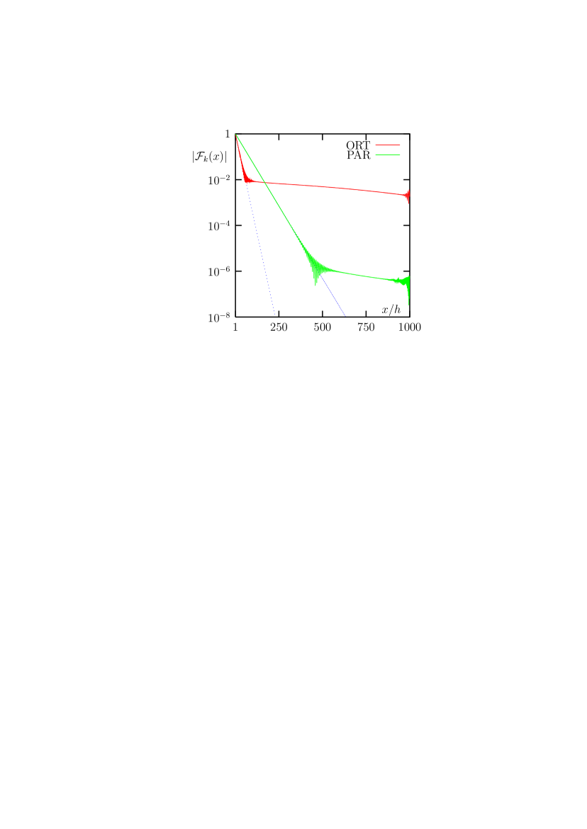
Figure 2: Propagation of a SP in an ordered chain of $N=1000$ nanospheres for orthogonal (ORT) and parallel (PAR) polarization of oscillations with respect to the chain. Parameters: $\omega=\omega_{\mathrm{F}}$, $\gamma/\omega_{\mathrm{F}}=0.002$, $\lambda=10h$, $h=4a$.

Mathematically, the relatively slow decay of the extraordinary SP can be understood as follows. First, note the the exponential decay of the ordinary SP is, in fact, the result of superposition of an infinite number of plane waves whose wave numbers are in the interval $\Delta q\propto\delta$. The corresponding wave packet decays spatially on scales $\ell\propto 1/\Delta q$. However, in the case of extraordinary SP, $\Delta q$ can not be defined since the corresponding resonance is non-Lorentizian. It can be, however, stated that the extraordinary SP is a superposition of plane waves whose wave numbers are very close to $k$. Since, however, the wavenumbers can still slightly deviate from $k$, some spatial decay at large distances can still occur.

The conclusion we can make so far is that the ordinary SP experiences exponential decay along the chain due to Ohmic losses in metal. This decay is very accurately described by the quasi-particle pole approximation. The extraordinary SP has, initially, much smaller amplitude than the ordinary one. This is because the peaks in Fig. 1 are very narrow. The quasi-particle pole approximation is invalid for the extraordinary SP and its decay is much less affected by Ohmic losses. As a result, the extraordinary SP decays at a much slower rate and, at sufficiently large propagation distance, begins to dominate. We also note that the extraordinary SP can be excited even for longitudinally-polarized SP, although its amplitude is smaller by some four orders of magnitude than for the case of transverse oscillations.

In Fig. 3, we illustrate the influence of Ohmic losses on SP propagation. Here we plot $|{\mathcal{F}}_{k}(x)|$ as a function of $x$ (sampled at $x=x_{n}$) for $\omega=\omega_{\mathrm{F}}$ and different values of the ratio $\gamma/\omega_{\mathrm{F}}$. First, in the absence of absorption ($\gamma=0$), the ordinary SP propagates along the chain without decay. Once we introduce absorption, the ordinary SP decays exponentially with the characteristic length scale $\ell$ given by (12). Note that, for the specific metal permeability model (6), $\ell\propto\omega_{\mathrm{F}}/\gamma$. Some dependence of the rate of decay of the extraordinary SP on the ratio $\gamma/\omega_{\mathrm{F}}$ is visible in the case of orthogonal polarization [Fig. 3(a)]. However, when the polarization is longitudinal [Fig. 3(b)], decay of the extraordinary SP is dominated by radiative losses. In particular, the slow-decaying segments of the curves for $\gamma/\omega_{\mathrm{F}}=0.002$ and $\gamma/\omega_{\mathrm{F}}=0.004$ in Fig. 3(b) coincide with high precision.

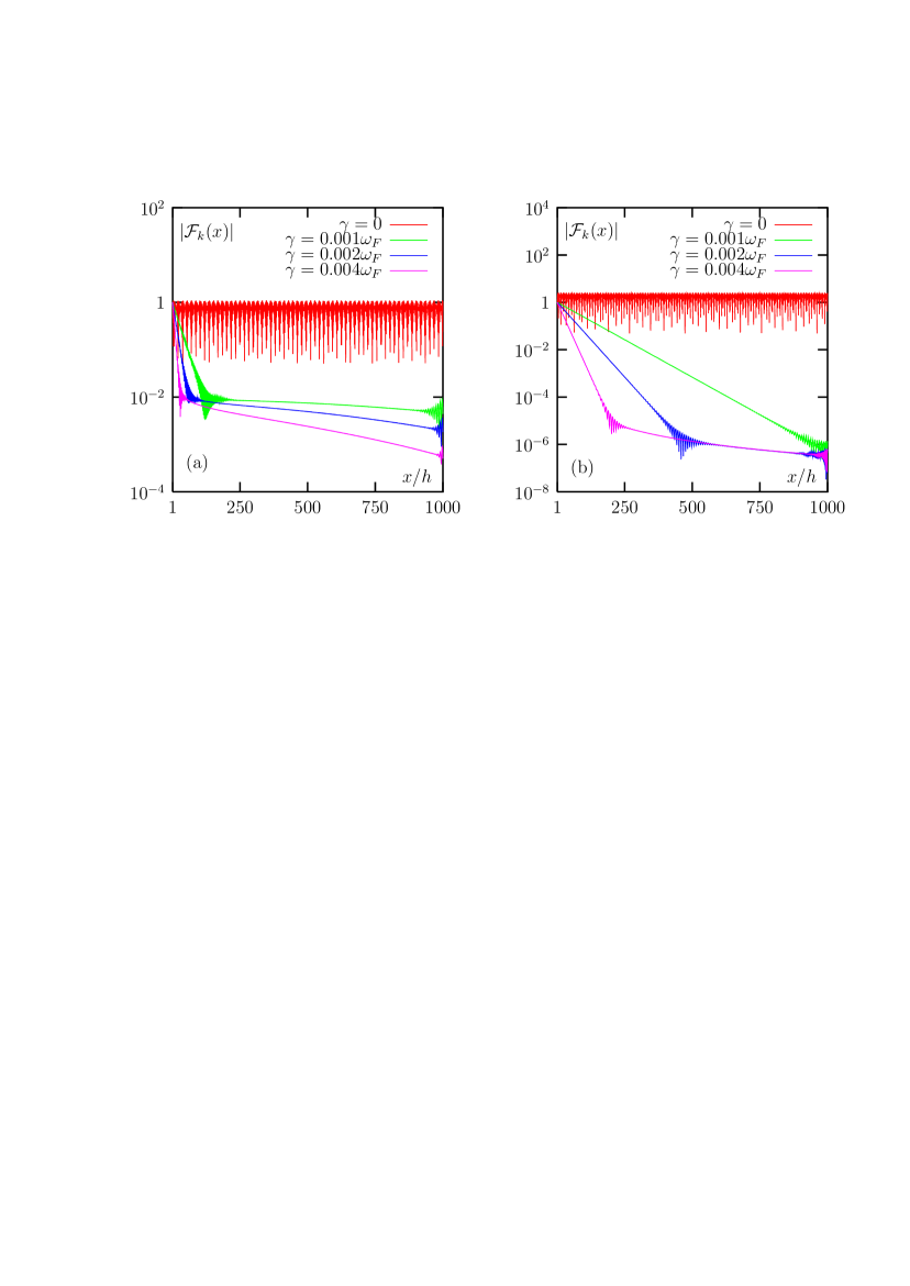
Figure 3: Same as in Fig. 3 for different ratios $\gamma/\omega_{\mathrm{F}}$ and for SP polarized orthogonally (a) and parallel (b) to the chain.

Next, we study SP propagation for different values of the ratio $\omega/\omega_{\mathrm{F}}$. As noted above, we assume the parameters $kh=\omega h/c=0.2\pi$ and $h/a=4$ to be fixed. Thus, $\omega/\omega_{\mathrm{F}}$ can vary either due to a change in $\omega_{\mathrm{F}}$ or due to a simultaneous change in $\omega$, $h$ and $a$ such that $\omega h=\mathrm{const}$ and $h/a=\mathrm{const}$. It follows from Fig. 1(a) that, for the selected set of parameters, the ordinary plasmon can be excited for $-0.89<h^{3}\mathrm{Re}(1/\alpha)<1.56$. This corresponds to $\omega/\omega_{\mathrm{F}}$ lying in the interval $0.988<\omega/\omega_{\mathrm{F}}<1.007$. In Fig. 4, we illustrate propagation of SP excitations for some values of $\omega/\omega_{\mathrm{F}}$ inside this interval, exactly at the lower and upper bounds of this interval, and slightly outside of the interval. Results are shown for two values of absorption strength: $\gamma/\omega_{\mathrm{F}}=0$ and $\gamma/\omega_{\mathrm{F}}=0.002$.

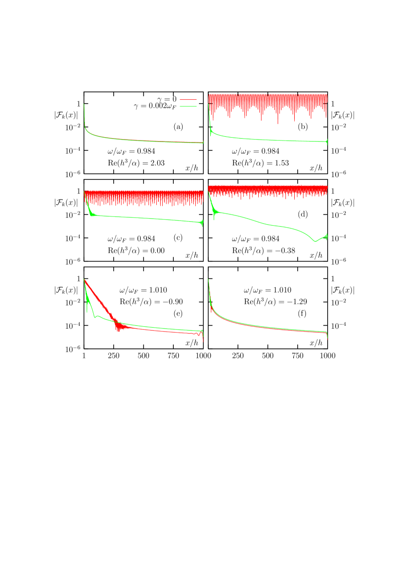
Figure 4: Same as in Fig. 3 for different ratios $\omega/\omega_{\mathrm{F}}$ and $\gamma/\omega_{\mathrm{F}}$, as indicated, and for SP polarized orthogonally to the chain.

First, consider the two cases when $\omega/\omega_{\mathrm{F}}$ is outside of the interval where the ordinary SP can be excited: $\omega/\omega_{\mathrm{F}}=0.984$ and $\omega/\omega_{\mathrm{F}}=1.010$ (correspondingly, $h^{3}\mathrm{Re}(1/\alpha)=2.03$ and $h^{3}\mathrm{Re}(1/\alpha)=-1.29$), shown in Fig. 4(a,f). In the case $\omega/\omega_{\mathrm{F}}=0.984$, the ordinary SP exhibits very fast spatial decay, which is characteristic for the noninteracting limit when $G_{k}(n,n_{0})\propto\delta_{n,n_{0}}$. After the initial decay of the ordinary SP, the extraordinary SP becomes dominating. The extraordinary SP decays slowly by means of radiative losses. It is interesting to note that decay of the extraordinary SP is almost unaffected by Ohmic losses in metal, although a noticeable dependence on $\gamma$ appears if we further increase the parameter $\gamma/\omega_{\mathrm{F}}$ by the factor of $10$ (data not shown). A qualitatively similar behavior is obtained at $\omega/\omega_{\mathrm{F}}=1.010$. However, the decay of extraordinary SP in this case is a little faster. Paradoxically, the curve corresponding to $\gamma/\omega_{\mathrm{F}}=0.002$ is slightly higher than the curve corresponding to $\gamma=0$ in Fig. 4(f) (similar peculiarity is seen in Fig. 4(e)).

When the ratio $\omega/\omega_{\mathrm{F}}$ is inside the interval where the ordinary SP can be excited [Fig. 4(c,d)], SP propagation is strongly influenced by absorptive losses. In the absence of such losses, the ordinary SP propagates along the chain indefinitely and dominates the extraordinary SP. However, in the presence of even small absorption, the ordinary SP decays exponentially so that, at sufficiently large propagation distances, the extraordinary SP starts to dominate. A qualitatively similar picture is also obtained for the borderline case $\omega/\omega_{\mathrm{F}}=0.984$ [Fig. 4(b)]. In the second borderline case [Fig. 4(e)], SP propagation is more complicated. The wave numbers of both ordinary and extraordinary SPs in this case are close to $k$, so that both can experience radiative decay, as is evident in the case of zero absorption.

To conclude this section, we note that propagation of SP excitations in long periodic chains can be characterized by exponential decay. This decay is caused either by absorptive or by radiative losses. At small propagation distances, energy is transported by the ordinary SP excitation, if the ordinary SP can be excited (e.g., if $\mathrm{Re}(1/\alpha)$ is inside the appropriate interval). However, at sufficiently large propagation distances, there is a cross over to transport by means of the extraordinary SP. In this case, propagation is mediated by far-zone interaction and is characterized by slow, radiative decay which is affected by absorptive losses only weakly.

We note that exponential decay in ordered chains, if exists, is not caused by Anderson localization, since we have not, so far, introduced disorder into the system. For example, as was discussed in section III, a linear superposition of delocalized plane wave modes of the form (9) can exhibit exponential decay with the characteristic length (12). The irreversible exponential decay is, in fact, obtained because the delocalized modes form a truly continuous spectrum (are indexed by a continuous variable $q$). Of course, any superposition of discrete delocalized modes would result in Poincare recurrences.

V Propagation in Disordered Chains

The ordinary (quasistatic) SP propagates in ordered chains without radiative losses due to the perfect periodicity of the lattice. However, once this periodicity is broken, the quasistatic SP can experience radiative losses and spatial decay even in the absence of absorption. Dependence of the radiative quality of SP modes in finite one-dimensional chains on disorder strength was studied in Ref. Burin et al., 2004. It was shown that position disorder tends to decrease the radiative quality factor of initially non-radiating (“bound”) modes. In this section we study how the disorder influences propagation of the SP along the chain and take a separate look at the ordinary and extraordinary SPs. We also consider two types of disorder: off-diagonal and diagonal. Off-diagonal disorder is disorder in particle positions while all particles are identical. Diagonal disorder arises due to differences in particle properties, even if the particle positions are perfectly ordered.

The exponential decay due to Ohmic losses in the material can mask the effects of disorder. Therefore, we assume in this section that the nanospheres are non-absorbing, i.e., set $\gamma_{n}=0$. Physically, absence of absorption can be realized by embedding the chain of nanoparticles in a transparent dielectric host medium with positive gain Sudarkin and Demkovich (1989); Bergman and Stockman (2003); Avrutsky (2004); Lawandy (2004). Such medium has dielectric permeability $\epsilon_{\mathrm{h}}$ with positive real and negative imaginary parts. The gain can be tuned so that the effective permeability of inclusions $\epsilon/\epsilon_{\mathrm{h}}$ is purely real and negative. We also work in the regime $kh=0.2\pi$, $h=4a$.

V.1 Off-Diagonal Disorder

Off-diagonal disorder is disorder in particle position. It is called “off-diagonal” because it affects only off-diagonal elements of the interaction matrix $G_{k}(x_{n},x_{n^{\prime}})$. In the simulations shown below, coordinates of particles in a disordered chain were taken to be $x_{n}=h(n+\xi_{n})$ where $\xi_{n}$ is a random variable evenly distributed in the interval $[-A,A]$. The random numbers $\xi_{n}$ are taken to be mathematically independent. Therefore, the disorder is uncorrelated.

The first example concerns propagation in an non-absorbing chain of $N=10,000$ nanospheres excited exactly at the Frohlich frequency $\omega=\omega_{\mathrm{F}}$. Numerical results for different levels of disorder are illustrated in Fig. 5 where we plot $|{\mathcal{F}}_{k}(x)|$ as a function of $x$ (sampled at $x=x_{n}$).

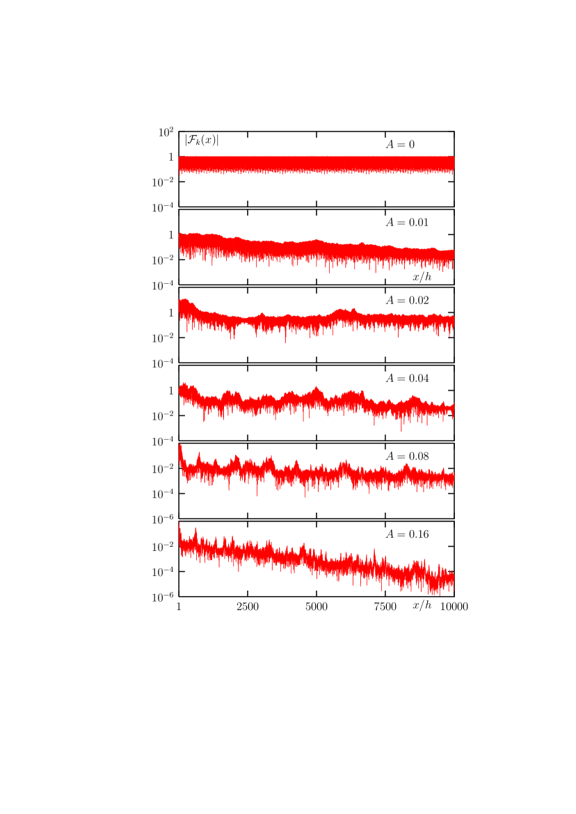
Figure 5: Propagation of SP in a chain of $N=10,000$ non-absorbing ($\gamma=0$) nanospheres for different levels of off-diagonal disorder $A$, as indicated. SP polarization is orthogonal to the chain. Other parameters: $kh=0.2\pi$, $\omega/\omega_{\mathrm{F}}=1$, $h/a=4$.

One obvious conclusion that can be made from inspection of Fig. 5 is that disorder causes spatial decay of SP. Since the system has no absorption, energy is lost to radiation. However, the exact law of decay strongly depends on particular realization of disorder. In Figs. 6 and 7, we plot the function $|{\mathcal{F}}_{k}(x)|$ for $A=0.01$ and $A=0.02$, respectively, and for three different realizations of disorder (without the use of logarithmic scale). Giant fluctuations in the amplitude of transmitted SP are quite apparent. In all cases, after some initial growth, the amplitude decays, although some random recurrences (due to re-excitation) can take place. However, the amplitude $|{\mathcal{F}}_{k}(x)|$ at a given site $x=x_{n}$ strongly depends on realization of disorder and can be very far from its ensemble average, even at very large propagation distances. Therefore, the function ${\mathcal{F}}_{k}(x)$ appears to be not self-averaging. In particular, any particular realization of the intensity ${\mathcal{I}}_{k}(x)=|{\mathcal{F}}_{k}(x)|^{2}$ does not satisfy either the radiative transport equation or the diffusion equation. The absence of transport and self-averaging is characteristic for Anderson localization. We note that the localization discussed here is an interference (radiative) effect which is different from localization of quasistatic polarization modes studied in Refs. Stockman et al., 2001; Genov et al., 2005. Localization properties of the eigenmodes in disordered chains is a subject of separate investigation and will be reported elsewhere.

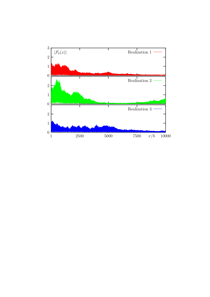
Figure 6: Propagation of SPs in a chain with off-diagonal disorder of amplitude $A=0.01$ for different random realizations of disorder. Other parameters same as in Fig. 5.

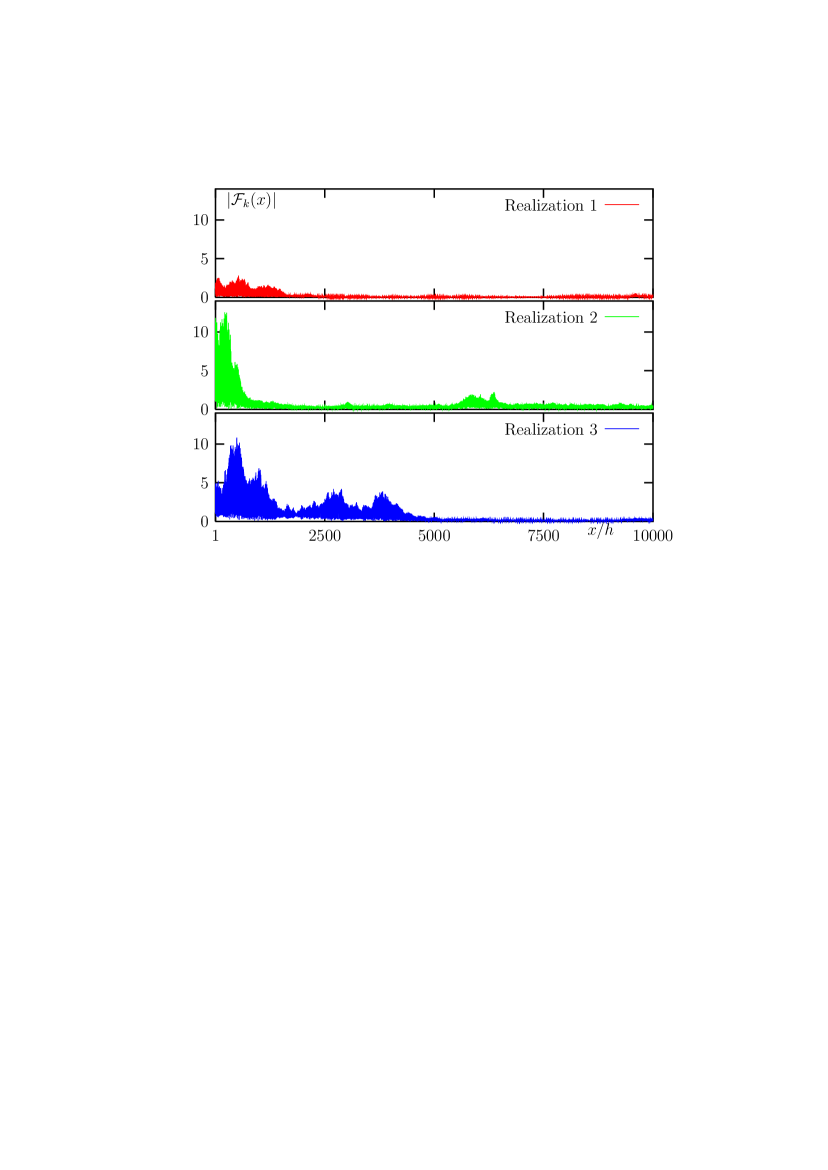
Figure 7: Same as in Fig. 6, but for $A=0.02$.

The situation is complicated by the presence of two types of SP excitations. One can argue that localization properties of these two types of SPs might be different. To investigate this possibility, we perform two types of numerical experiments. First, we repeat simulations illustrated in Fig. 5 but for $\omega/\omega_{\mathrm{F}}=0.948$. In this case, the ordinary SP is not excited in ordered chains (see Fig. 4(a)). Results are shown in Fig. 8 . It can be concluded from the figure that off-diagonal disorder does not result in additional decay of the extraordinary SP. In fact, the curves with $A=0$, $A=0.1$ and $A=0.04$ are indistinguishable. This should be contrasted with the case $\omega/\omega_{\mathrm{F}}=1$, when, at the level of disorder $A=0.02$, spatial decay is already well manifested. The conclusion one can make is that the extraordinary SP excitations do not experience localization due to uncorrelated off-diagonal disorder in the chain. Therefore, spatial decay seen in Figs. 5 and 7 is decay of the ordinary SP. At very large propagation distances, ${\mathcal{F}}_{k}(x)$ continues to oscillate around the baseline of the extraordinary SP.

Figure 8: Same as in Fig. 5 but for $\omega/\omega_{\mathrm{F}}=0.984$ and for different levels $A$ of off-diagonal disorder, as indicated. Note that the curves for $A=0$ and $A=0.01$ and $A=0.04$ are indistinguishable.

The second numerical experiment that can elucidate the influence of disorder on ordinary and extraordinary SPs is simulation of an extinction measurement when the chain is excited, instead of a nera-field tip, by a plane wave $E_{0}\exp(iqx)$. Namely, we will look at the dependence of the specific (per one nanosphere) extinction cross section $\sigma_{e}$ on $q$. There are two different experimental setups that can be used to measure $\sigma_{e}(q)$. When $q$ is in the interval $0\leq q<k$, this experiment can be carried out simply by varying the angle between the incident beam and the chain. However, values $q>k$ are not accessible in this experiment. In this case, the chain can be placed on a dielectric substrate and excited by evanescent wave originating due to the total internal reflection of the incident beam. The maximum longitudinal wave number of the evanescent wave is $nk$, where $n>1$ is the refractive index of the substrate. We note that it is not realistically possible to access all wave numbers up to $q=\pi/h$ in this way because, in the particular case $kh=0.2\pi$, this would require the refractive index $n=5$. Refractive indices of such magnitude are not achievable in the optical range. However, in a numerical simulation, we can assume that a hypothetical transparent substrate with $n=5$ exists. Besides, all wave numbers $q$ in the first Brillouin zone of the lattice can be accessible for a different choice of parameters (particularly, for larger values of $kh$).

The specific extinction $\sigma_{e}(q)$ is given by the following formula:

$$\sigma_{e}(q)=\frac{4\pi k}{N|E_{0}|^{2}}\sum_{n=1}^{N}E_{0}^{*}\exp(-iqx_{n})d_{n}\ ,$$ (15)

where $d_{n}$ is the solution to Eq. (1) with the right-hand side $E_{n}=E_{0}\exp(iqx_{n})$. In Fig. 9, we plot the dimensionless quantity $h^{-2}\sigma_{e}(q)$ as a function of $q$ for transverse oscillations in partially disordered non-absorbing chains. Two peaks are clearly visible in the spectrum. The first peak at $q=q_{1}\approx 0.47\pi/h$ corresponds to excitation of the ordinary SP. The second peak at $q=q_{2}\approx k$ corresponds to excitation of the extraordinary SP. In infinite, periodic and non-absorbing chains, the spectrum has a simple pole at $q=q_{1}$. fn (4) In the finite chain with $N=10,000$, the singularity is replaced by a very sharp maximum. Introduction of even slight disorder tends to further broaden and randomize this peak. Obviously, this broadening, as well as the randomization of the spectrum in the vicinity of $q=q_{1}$, result in spatial decay of the ordinary SP excitated by a near-field tip. However, the peak corresponding to the extraordinary SP is almost unaffected by disorder. Consequently, the extraordinary SP does not experience localization and related spatial decay when off-diagonal disorder is introduced into the system.

Figure 9: Specific extinction $\sigma_{e}$ as a function of lateral wave number of incident wave, $q$, for different levels of off-diagonal disorder, $A$.

The physical reason why the extraordinary SP is not affected by disorder is quite straightforward. This SP is mediated by electromagnetic waves in the far (radiation) zone that arrive at a given nanosphere from all other nanospheres. The synchronism condition (that all these secondary waves arrive in phase) is not affected by disorder as long as the displacement amplitudes $\xi_{n}$ are small compared to the wavelength. In the numerical examples of this section, wavelength is ten times larger than the inter-particle spacing, which is, in turn, much larger than the displacement amplitudes. Additionally, effects of disorder are expected to be averaged if the amplitudes $\xi_{n}$ are mathematically independent because the scattered field at a given nanosphere is a sum of very large number of secondary waves. In contrast, the ordinary SP is mediated by near-field interactions which are very sensitive to even slight displacements of nanospheres. Besides, the scattered field at a given nanosphere (when the ordinary SP propagates in the chain) is a rapidly converging sum of secondary fields, so that only a few terms in this sum are important and no effective averaging takes place.

V.2 Diagonal Disorder

Diagonal disorder is disorder in the properties of nanospheres. There are several possibilities for introducing such disorder.

First, the spheres can be polydisperse, i.e., have different radiuses $a_{n}$. This is, however, not a truly diagonal disorder. Indeed, polarizability of $n$-th nanosphere can be written in this case as $f_{n}\langle\alpha\rangle$ where $f_{n}=(a_{n}/\langle a\rangle)^{3}$ and $\langle a\rangle$ is the average radius (note that the radiative correction to $1/\alpha_{n}$ can be included into the dipole sum $S(k,q)$, so that this analysis remains valid even when this correction is important). The factors $f_{n}$ are all positive-definite which allows one to introduce a simple transformation of Eq. (1) which removes the diagonal disorder Perminov et al. (2004). Then the disorder becomes effectively off-diagonal. More importantly, one can retain a well-defined spectral parameter of the theory, $1/\langle\alpha\rangle$. We, therefore, do not consider polydispersity in this section.

The second possibility is variation of the absorptive parameter $\gamma$. This effect that can be practically important. Yet, we are interested in propagation in the absence of Ohmic losses and, therefore, set $\gamma_{n}=0$.

The third, and the most fundamental, reason for diagonal disorder is variation of the Frohlich frequency of nanospheres. Namely, we take the Frohlich frequency of the $n$-th particle to be $\omega_{\mathrm{F}n}=\langle\omega_{\mathrm{F}}\rangle(1+\xi_{n})$, where $\xi_{n}$ are statistically independent random variables evenly distributed in the interval $[-A,A]$ and $\omega/\langle\omega_{\mathrm{F}}\rangle=1$. The factors $f_{n}$ in this case are no longer positive-definite and the transformation of Ref. Perminov et al., 2004 can not be applied. The most profound consequence of introducing the diagonal disorder is that the spectral parameter such as $1/\alpha$ is no longer well defined. As long as the disorder amplitude is relatively small, one can view $1/\langle\alpha\rangle$ as an approximate spectral parameter. However, as the amplitude of disorder increases, this approach becomes invalid. We have seen in section IV that variation of the ratio $\omega/\omega_{\mathrm{F}}$ in the interval $0.988<\omega/\omega_{\mathrm{F}}<1.007$ can result in dramatic changes in the way an SP excitation propagates along the chain. For $\omega/\omega_{\mathrm{F}}$ outside of this interval, ordinary SP could not be effectively excited. However, in section IV, variation of $\omega/\omega_{\mathrm{F}}$ applied to all nanospheres simultaneously. We now introduce random uncorrelated variation of this ratio for each individual nanosphere. The effects of such disorder are difficult to predict theoretically. We can, however, expect that these effects become dramatic for $A\gtrsim 0.01$ since, in this case, the ratio $\omega/\omega_{\mathrm{F}n}$ can be outside of the interval $[0.988,1.007]$.

We first adduce in Fig. 10 the same dependencies as shown in Fig. 5 but for different levels of diagonal disorder. The results appear to be, qualitatively, quite similar, although in the case $A=0.016$, there is no visible trend for $x/h>3000$. We then investigate whether the extraordinary SP remains insensitive to diagonal disorder. Data analogous to those shown in Fig. 8, but for diagonal disorder, are presented in Fig. 11. It can be seen that the influence of diagonal disorder on the extraordinary SP is stronger than that of the off-diagonal disorder. When the disorder amplitude $A$ exceeds $0.01$, the influence becomes quite dramatic. But paradoxically, at $A=0.016$, the average decay rate is much slower than for $A=0.008$, although the amplitude of fluctuations is much larger.

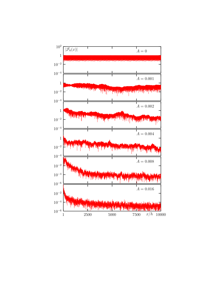
Figure 10: Same as in Fig. 5, but for different levels $A$ of diagonal disorder.

Figure 11: Same as in Fig. 10 but for $\omega/\omega_{\mathrm{F}}=0.984$ and for different levels $A$ of off-diagonal disorder, as indicated. Note that the curves for $A=0$ and $A=0.01$ are indistinguishable.

To see why this happens, we look at the extinction spectra $\sigma_{e}(q)$. These are plotted in Fig. 12. The fundamental difference between the off-diagonal and diagonal disorder is clearly revealed by comparing this figure to Fig. 9. Namely, the effect of diagonal disorder is not only to broaden and randomize the peak at $q=q_{1}$, but also to shift it towards the peak corresponding to the extraordinary SP. At sufficiently large levels of disorder ($A\geq 0.016$), the separate peaks disappear and a broad structure emerges. At this point, ordinary and extraordinary SP can no longer be distinguished. Correspondingly, the ordinary and extraordinary SP are effectively mixed in the $A=0.016$ curve in Fig. 11, while fo smaller amplitudes of the diagonal disorder, the extraordinary SP is excited predominatlly.

Figure 12: Specific extinction $\sigma_{e}$ as a function of lateral wave number of incident wave, $q$, for different levels of off-diagonal disorder, $A$.

VI Summary

We have considered surface plasmon (SP) propagation in a linear chain of metal nanoparticles. Computer simulations reveal the existence of two types of plasmons: ordinary (quasistatic) and extraordinary (non-quasistatic) SPs.

The ordinary SP is characterized by short-range interaction of nanospheres in a chain. The retardation effects are inessential for its existence and properties. The ordinary SP behaves as a quasistatic excitation. The ordinary SP can not radiate into the far zone in perfectly periodic chains because its wave number is larger than the wavenumber $k=\omega/c$ of free electromagnetic waves. However, it can experience decay due to absorptive dissipation in the material.

The second, extraordinary, SP propagates due to long-range (radiation zone) interaction in a chain. Its excitation is possible due to the existence of the non-Lorentzian optical resonance in the chain introduced in Ref. Markel, 2005. The extraordinary SP may experience some radiative loss but is much less afected by absorptive dissipation and disorder. As a result, it can propagate to much larger distances along the chain. The extraordinary SP can be used to guide energy or information in all-optical integrated photonic systems.

We have also considered the effects of disorder and localization of the ordinary and extraordinary SPs. Results of numerical simulations suggest that even small disorder in the position or properties of nanoparticles results in localization of the ordinary SP. However, the extraordinary SP appears to remain delocalized for all types and levels of disorder considered in the paper.

The authors can be reached at vmarkel@mail.med.upenn.edu (VAM) and asarychev@ethertronics.com (AKS).

References

- Sarychev and Shalaev (2000) A. K. Sarychev and V. M. Shalaev, Phys. Rep. 335, 275 (2000).
- Stockman (2004) M. I. Stockman, Phys. Rev. Lett. 93(13), 137404 (2004).
- Engheta et al. (2005) N. Engheta, A. Salandrino, and A. Alu, Phys. Rev. Lett. 95(9), 095504 (2005).
- Podolskiy et al. (2002) V. A. Podolskiy, A. K. Sarychev, and V. M. Shalaev, Laser Phys. 12, 292 (2002).
- Stockman et al. (2004) M. I. Stockman, D. J. Bergman, and T. Kobayashi, Phys. Rev. B 69, 054202 (2004).
- Quinten et al. (1998) M. Quinten, A. Leitner, J. R. Krenn, and F. R. Ausennegg, Opt. Lett. 23(17), 1331 (1998).
- Brongersma et al. (200) M. L. Brongersma, J. W. Hartman, and H. A. Atwater, Phys. Rev. B 62(24), R16356 (2000).
- Burin et al. (2004) A. L. Burin, H. Cao, G. C. Schatz, and M. A. Ratner, J. Opt. Soc. Am. B 21(1), 121 (2004).
- Quidant et al. (2004) R. Quidant, C. Girard, J.-C. Weeber, and A. Dereux, Phys. Rev. B 69, 085407 (2004).
- Simovski et al. (2005) C. R. Simovski, A. J. Viitanen, and S. A. Tretyakov, Phys. Rev. E 72, 066606 (2005).
- Maier et al. (2003) S. A. Maier, P. G. Kik, H. A. Atwater, S. Meltzer, E. Harel, B. E. Koel, and A. G. Requicha, Nature Materials 2, 229 (2003).
- Guillon (2006) M. Guillon, Opt. Express 14(7), 3045 (2006).
- Markel (1993) V. A. Markel, J. Mod. Opt. 40(11), 2281 (1993).
- Zou et al. (2004) S. Zou, N. Janel, and G. C. Schatz, J. Chem. Phys. 120(23), 10871 (2004).
- Zou and Schatz (2006) S. Zou and G. C. Schatz, Nanotechnology 17, 2813 (2006).
- Markel (2005) V. A. Markel, J. Phys. B 38, L115 (2005).
- Weber and Ford (2004) W. H. Weber and G. W. Ford, Phys. Rev. B 70, 125429 (2004).
- Citrin (2005) D. S. Citrin, Nano Letters 5(5), 985 (2005).
- Citrin (2006) D. S. Citrin, Opt. Lett. 31(1), 98 (2006).
- Draine (1988) B. T. Draine, Astrophys. J. 333, 848 (1988).
- fn (2) To the first order in , where is the wavenumber such that .
- fn (3) In general, resonances take place at , where is an arbitrary integer, with the restriction that must be in the first Brillouin zone of the lattice, . If , as is the case in this paper, the only possible solutions are .
- fn (1) Strictly speaking, there may be two solutions rather than one, since the curve can cross zero at two separate points. This happens in Fig. 1(a) for . However, since the peaks are exponentially narrow, the physical effect of exciting two SP with slightly different wave numbers is not expected to be physically observable.
- Sansonetti and Furdyna (1980) J. E. Sansonetti and J. K. Furdyna, Phys. Rev. B 22(6), 2866 (1980).
- Park and Stroud (2004) S. Y. Park and D. Stroud, Phys. Rev. B 69, 125418 (2004).
- Markel et al. (2004) V. A. Markel, V. N. Pustovit, S. V. Karpov, A. V. Obuschenko, V. S. Gerasimov, and I. L. Isaev, Phys. Rev. B 70(5), 054202 (2004).
- Sudarkin and Demkovich (1989) A. N. Sudarkin and P. A. Demkovich, Sov. Phys. Tech. Phys. 34, 764 (1989).
- Bergman and Stockman (2003) D. J. Bergman and M. I. Stockman, Phys. Rev. Lett. 90(2), 027402 (2003).
- Avrutsky (2004) I. Avrutsky, Phys. Rev. B 70(15), 155416 (2004).
- Lawandy (2004) N. M. Lawandy, Appl. Phys. Lett. 85(21), 5040 (2004).
- Stockman et al. (2001) M. I. Stockman, S. V. Faleev, and D. J. Bergman, Phys. Rev. Lett. 87(16), 167401 (2001).
- Genov et al. (2005) D. A. Genov, V. M. Shalaev, and A. K. Sarychev, Phys. Rev. B 72, 113102 (2005).
- fn (4) The singularity is integrable if we adopt the usual rule for bypassing the pole. Namely, the pole position at corresponds to .
- Perminov et al. (2004) S. V. Perminov, S. G. Rautian, and V. P. Safonov, J. Exp. Theor. Phys. 98(4), 691 (2004).