Simple Viscous Flows: From Boundary Layers to the Renormalization Group

Abstract

The seemingly simple problem of determining the drag on a body moving through a very viscous fluid has, for over 150 years, been a source of theoretical confusion, mathematical paradoxes, and experimental artifacts, primarily arising from the complex boundary layer structure of the flow near the body and at infinity. We review the extensive experimental and theoretical literature on this problem, with special emphasis on the logical relationship between different approaches. The survey begins with the developments of matched asymptotic expansions, and concludes with a discussion of perturbative renormalization group techniques, adapted from quantum field theory to differential equations. The renormalization group calculations lead to a new prediction for the drag coefficient, one which can both reproduce and surpass the results of matched asymptotics.

I INTRODUCTION TO LOW $R$ FLOW

I.1 Overview

In 1851, shortly after writing down the Navier-Stokes equations, Sir George Gabriel Stokes turned his attention to what modern researchers might whimsically refer to as “the hydrogen atom” of fluid mechanics: the determination of the drag on a sphere or an infinite cylinder moving at fixed speed in a highly viscous fluid Stokes (1851). Just as the quantum theory of the hydrogen atom entailed enormous mathematical difficulties, ultimately leading to the development of quantum field theory, the problem posed by Stokes has turned out to be much harder than anyone could reasonably have expected: it took over 100 years to obtain a justifiable lowest order approximate solution, and that achievement required the invention of a new branch of applied mathematics, matched asymptotic expansions. And just as the fine structure of the hydrogen atom’s spectral lines eventually required renormalization theory to resolve the problems of “infinities” arising in the theory, so too, Stokes’ problem is plagued by divergences that are, to a physicist, most naturally resolved by renormalization group theory Feynman (1948); Schwinger (1948); Tomonaga (1948); Stuckelberg and Petermann (1953); Gell-Mann and Low (1954); Wilson (1971a, b, 1983); Chen et al. (1996).

In order to appreciate the fundamental difficulty of such problems, and to expose the similarity with familiar problems in quantum electrodynamics, we need to explain how perturbation theory is used in fluid dynamics. Every flow that is governed by the Navier-Stokes equations only (i.e. the transport of passive scalars, such as temperature, is not considered; there are no rotating frames of reference or other complications) is governed by a single dimensionless parameter, known as the Reynolds number, which we designate as $R$. The Reynolds number is a dimensionless number made up of a characteristic length scale $L$, a characteristic velocity of the flow $U$, and the kinematic viscosity $\nu\equiv\eta/\rho$, where $\eta$ is the viscosity and $\rho$ is the density of the fluid. In the problems at hand, defined precisely below, the velocity scale is the input fluid velocity at infinity, $u_{\infty}$, and the length scale is the radius $a$ of the body immersed in the fluid. Then the Reynolds number is given by:

$$R\equiv\frac{u_{\infty}a}{\nu}$$ (1)

The Reynolds number is frequently interpreted as the ratio of the inertial to viscous terms in the Navier-Stokes equations. For very viscous flows, $R\rightarrow 0$, and so we anticipate that a sensible way to proceed is perturbation theory in $R$ about the problems with infinite viscosity, i.e. $R=0$. In this respect, the unwary reader might regard this as an example very similar to quantum electrodynamics, where the small parameter is the fine structure constant. However, as we will see in detail below, there is a qualitative difference between a flow with $R=0$ and a flow with $R\rightarrow 0$. The fundamental reason is that by virtue of the circular or spherical geometry, the ratio of inertial to viscous forces in the Navier-Stokes equations is not a constant everywhere in space: it varies as a function of radial distance $r$ from the body, scaling as $\mathcal{O}\left(Rr/a\right)$. Thus, when $R=0$, this term is everywhere zero; but for any non-zero $R$, as $r/a\rightarrow\infty$ the ratio of inertial to viscous forces becomes arbitrarily large. Thus, inertial forces can not legitimately be regarded as negligible with respect to viscous forces everywhere: the basic premise of perturbation theory is not valid.

Perturbation theory has to somehow express, or manifest, this fact, and it registers its objection by generating divergent terms in its expansion. These divergences are not physical, but are the perturbation theory’s way of indicating that the zeroth order solution—the point about which perturbation theory proceeds—is not a correct starting point. The reader might wonder if the precise nature of the breakdown of perturbation theory, signified by the divergences, can be used to deduce what starting point would be a valid one. The answer is yes: this procedure is known as the perturbative renormalization group (RG), and we will devote a significant fraction of this article to expounding this strategy. As most readers will know, renormalization Feynman (1948); Schwinger (1948); Tomonaga (1948) and renormalization group Stuckelberg and Petermann (1953); Gell-Mann and Low (1954); Wilson (1971a, b, 1983) techniques in quantum field theories have been stunningly successful. In the most well-controlled case, that of quantum electrodynamics, the smallness of the fine structure constant allows agreement of perturbative calculations with high-precision measurements to 12 significant figures Gabrielse et al. (2006). Do corresponding techniques work as well in low Reynolds fluid dynamics, where one wishes to calculate and measure the drag $C_{D}$ (defined precisely below)? Note that in this case, it is the functional form in $R$ for the drag that is of interest, rather than the drag at one particular value of $R$, so the measure of success is rather more involved. Nevertheless, we will see that calculations can be compared with experiments, but there too will require careful interpretation.

Historically a different strategy was followed, leading to a set of techniques known generically as singular perturbation theory, in particular encompassing boundary layer theory and the method of matched asymptotic expansions. We will explain these techniques, developed by mathematicians starting in the 1950’s, and show their connection with renormalization group methods.

Although the calculational techniques of matched asymptotic expansions are widely regarded as representing a systematically firm footing, their best results apply only to infinitesimally small Reynolds number. As shown in Figure 1, the large deviations between theory and experiment for $R\sim 0.5$ demonstrate the need for theoretical predictions which are more robust for small but non-infinitesimal Reynolds numbers. Ian Proudman, who, in a tour de force helped obtain the first matched asymptotics result for a sphere Proudman and Pearson (1957), expressed it this way: “It is therefore particularly disappointing that the numerical ‘convergence’ of the expansion is so poor.” Chester and Breach (1969) In spite of its failings, Proudman’s solution from 1959 was the first mathematically rigorous one for flow past a sphere; all preceding theoretical efforts were worse.

\psfrag{Re}{$R=U_{\infty}a/\nu$}\psfrag{CD}{$C_{D}R/4\pi$}\psfrag{Jayaweera XXXXXX}{Jayaweera}\psfrag{Tritton}{Tritton}\psfrag{Kaplun}{Eqn. \ref{cylinder:KaplunCD}}\includegraphics[width=214.2097pt]{fig1a}

\psfrag{Re}{$R=U_{\infty}a/\nu$}\psfrag{CD}{$C_{D}R/4\pi$}\psfrag{Jayaweera XXXXXX}{Jayaweera}\psfrag{Tritton}{Tritton}\psfrag{Kaplun}{Eqn. \ref{cylinder:KaplunCD}}\psfrag{Re}{$R=U_{\infty}a/\nu$}\psfrag{CD}{$C_{D}R/6\pi-1$}\psfrag{Maxworthy XXXXXX}{Maxworthy}\psfrag{Le Clair}{Le Clair}\psfrag{Dennis}{Dennis}\psfrag{Chester and}{Eqn. \ref{matchedcd}}\includegraphics[width=214.2097pt]{fig1b}

Figure 1: (Color online) Comparing experiment with “state of the art” theoretical predictions for a sphere Jayaweera and Mason (1965); Tritton (1959) (right) and a cylinder Dennis and Walker (1971); Maxworthy (1965); Le Clair and Hamielec (1970) (left).

Further complicating matters, the literature surrounding these problems is rife with “paradoxes”, revisions, ad-hoc justifications, disagreements over attribution, mysterious factors of two, conflicting terminology, non-standard definitions, and language barriers. Even a recent article attempting to resolve this quagmire Lindgren (1999) contains an inaccuracy regarding publication dates and scientific priority. This tortured history has left a wake of experiments and numerical calculations which are of widely varying quality, although they can appear to agree when not examined closely. For example, it turns out that the finite size of experimental systems has a dramatic effect on measurements and simulations, a problem not appreciated by early workers.

Although in principle the matched asymptotics results can be systematically extended by working to higher order, this is not practical. The complexity of the governing equations prohibits further improvement. We will show here that techniques based on the renormalization group ameliorate some of the technical difficulties, and result in a more accurate drag coefficient at small but non-infinitesimal Reynolds numbers. Given the historical importance of the techniques developed to solve these problems, we hope that our solutions will be of general methodological interest.

We anticipate that some of our readers will be fluid dynamicists interested in assessing the potential value of renormalization group techniques. We hope that this community will see that our use of the renormalization group is quite distinct from applications to stochastic problems, such as turbulence, and can serve a different purpose. The second group of readers may be physicists with a field theoretic background, encountering fluids problems for the first time, perhaps in unconventional settings, such as heavy ion collisions and QCD Ackermann et al. (2001); Csernai et al. (2005); Heniz (2005); Hirano and Gyulassy (2006); Baier et al. (2006); Csernai et al. (2006) or 2D electron gases Stone (1990); Eaves (1998). We hope that this review will expose them to the mathematical richness of even the simplest flow settings, and introduce a familiar conceptual tool in a non-traditional context.

This review has two main purposes. The first purpose of the present article is to attempt a review and synthesis of the literature, sufficiently detailed that the subtle differences between different approaches are exposed, and can be evaluated by the reader. This is especially important, because this is one of those problems so detested by students, in which there are a myriad of ways to achieve the right answer for the wrong reasons. This article highlights all of these.

A second purpose of this article is to review the use of renormalization group techniques in the context of singular perturbation theory, as applied to low Reynolds number flows. These techniques generate a non-trivial estimate for the functional form of $C_{D}(R)$ that can be sensibly used at moderate values of $R\sim\mathcal{O}\left(1\right)$, not just infinitesimal values of $R$. As $R\rightarrow 0$, these new results reduce to those previously obtained by matched asymptotic expansions, in particular accounting for the nature of the mathematical singularities that must be assumed to be present for the asymptotic matching procedure to work.

Renormalization group techniques were originally developed in the 1950’s to extend and improve the perturbation theory for quantum electrodynamics. During the late 1960’s and 1970’s, renormalization group techniques famously found application in the problem of phase transitions Wilson (1971a); L. P. Kadanoff (1966); Widom (1963). During the 1990’s, renormalization group techniques were developed for ordinary and partial differential equations, at first for the analysis of nonequilibrium (but deterministic) problems which exhibited anomalous scaling exponents Goldenfeld et al. (1990); Chen et al. (1991) and subsequently for the related problem of travelling wave selection Chen et al. (1994c, a); Chen and Goldenfeld (1995). The most recent significant development of the renormalization group—and the one that concerns us here—was the application to singular perturbation problems Chen et al. (1994b); Chen et al. (1996). The scope of Chen et al. (1996) encompasses boundary layer theory, matched asymptotic expansions, multiple scales analysis, WKB theory, and reductive perturbation theory for spatially-extended dynamical systems. We do not review all these developments here, but focus only on the issues arising in the highly pathological singularities characteristic of low Reynolds number flows. For a pedagogical introduction to renormalization group techniques, we refer the reader to Goldenfeld (1992), in particular Chapter 10 which explains the connection between anomalous dimensions in field theory and similarity solutions of partial differential equations. We mention also that the RG techniques discussed here have also been the subject of rigorous analysis Bricmont and Kupiainen (1995); Bricmont et al. (1994); Moise et al. (1998); Ziane (2000); Moise and Temam (2000); Moise and Ziane (2001); Blomker et al. (2002); Lan and Lin (2004); Wirosoetisno et al. (2002); Petcu et al. (2005) in other contexts of fluid dynamics, and have also found application in cavitation Josserand (1999) and cosmological fluid dynamics Iguchi et al. (1998); Nambu and Yamaguchi (1999); Nambu (2000); Belinchon et al. (2002); Nambu (2002).

This review is organized as follows. After precisely posing the mathematical problem, we review all prior theoretical and experimental results. We identify the five calculations and measurements which are accurate enough, and which extend to sufficiently small Reynolds number, to be useful for evaluating theoretical predictions. Furthermore, we review the history of all theoretical contributions, and clearly present the methodologies and approximations behind previous solutions. In doing so, we eliminate prior confusion over chronology and attribution. We conclude by comparing the best experimental results with our new, RG-based, theoretical prediction. This exercise makes the shortcomings that Proudman lamented clear.

I.2 Mathematical formulation

The goal of these calculations is to determine the drag force exerted on a sphere and on an infinite cylinder by steady, incompressible, viscous flows. The actual physical problem concerns a body moving at constant velocity in an infinite fluid, where the fluid is at rest in the laboratory frame. In practice, it is more convenient to analyze the problem using an inertial frame moving with the fixed body, an approach which is entirely equivalent.

\psfrag{UInfinity}{$\vec{u}_{\infty}$}\psfrag{a}{$a$}\psfrag{r}{$r$}\psfrag{q}{$\theta$}\includegraphics*[width=151.76964pt]{fig2}

Figure 2: (Color online) Schematic for flow past a sphere or cylinder.

Flow past a sphere or circle is shown schematically in Figure 2. The body has a characteristic length scale, which we have chosen to be the radius ($a$), and it is immersed in uniform stream of fluid. At large distances, the undisturbed fluid moves with velocity $\vec{u}_{\infty}$.

The quantities shown in Table 1 characterize the problem. We assume incompressible flow, so $\rho=$ const.

Quantity	Description
$\vec{r}$	Coordinate Vector
$\vec{u}(\vec{r})$	Velocity Field
$\rho$	Fluid Density
$p(\vec{r})$	Pressure
$\nu$	Kinematic Viscosity
$a$	Characteristic Length of Fixed Body
$\vec{u}_{\infty}$	The Uniform Stream Velocity

Table 1: Quantities needed to characterize low $R$ flow past a rigid body.

The continuity equation (Eqn. 2) and the time-independent Navier-Stokes equations (Eqn. 3) govern steady-state, incompressible flow.

$$\nabla\cdot\vec{u}=0$$ (2)

$$(\vec{u}\cdot\nabla\vec{u})=-\frac{\nabla p}{\rho}+\nu\nabla^{2}\vec{u}$$ (3)

These equations must be solved subject to two boundary conditions, given in Eqn. 4. First, the no-slip conditions are imposed on the surface of the fixed body (Eqn. 4a). Secondly, the flow must be a uniform stream far from the body (Eqn. 4b). To calculate the pressure, one also needs to specify an appropriate boundary condition (Eqn. 4c), although as a matter of practice this is immaterial, as only pressure differences matter when calculating the drag coefficient.

$$\vec{u}(\vec{r}) = 0\quad\vec{r}\in\textrm{\{Surface of Fixed Body\}}$$ (4a)

$$\lim_{|\vec{r}|\to\infty}\vec{u}(\vec{r}) = \vec{u}_{\infty}$$ (4b)

$$\lim_{|\vec{r}|\to\infty}p(\vec{r}) = p_{\infty}$$ (4c)

It is convenient to analyze the problem using non-dimensional quantities, which are defined in Table 2.

Dimensionless Quantity	Definition
$\vec{r}^{*}$	$\vec{r}/a$
$\vec{u}^{*}(\vec{r})$	$\vec{u}(\vec{r})/|\vec{u}_{\infty}|$
$p^{*}(\vec{r})$	$a\ p(\vec{r})/\rho\ \nu\ |\vec{u}_{\infty}|$
$\vec{\nabla}^{*}$	$a\ \vec{\nabla}$

Table 2: Dimensionless variables.

When using dimensionless variables, the governing equations assume the forms given in Eqns. 5 and 6, where we have introduced the Reynolds Number, $R=|\vec{u}_{\infty}|a/\nu$, and denoted scaled quantities by an asterisk.

$$\nabla^{*}\cdot\vec{u^{*}}=0$$ (5)

$$R(\vec{u}^{*}\cdot\nabla^{*})\vec{u}^{*}=-\nabla^{*}p^{*}+\nabla^{*2}\vec{u}^{*}$$ (6)

The boundary conditions also transform, and will later be given separately for both the sphere and the cylinder (Eqns. 14, 10). Henceforth, the ^∗ will be omitted from our notation, except when dimensional quantities are explicitly introduced. It is useful to eliminate pressure from Eqn. 6 by taking the curl and using the identity $\nabla\times\nabla p=0$, leading to

$$(\vec{u}\cdot\nabla)(\nabla\times\vec{u})-((\nabla\times\vec{u})\cdot\vec{u})=\frac{1}{R}\nabla^{2}(\nabla\times\vec{u})$$ (7)

I.2.1 Flow past a cylinder

For the problem of the infinite cylinder, it is natural to use cylindrical coordinates, $\vec{r}=(r,\theta,z)$. We examine the problem where the uniform flow is in the $\hat{x}$ direction (see Figure 2). We will look for 2-d solutions, which satisfy $\partial_{z}{\vec{u}}=0$.

Since the problem is two dimensional, one may reduce the set of governing equations (Eqns. 5 and 6) to a single equation involving a scalar quantity, the Lagrangian stream function, usually denoted $\psi(r,\theta)$. It is defined by Eqn. 8.

$$u_{r}=\frac{1}{r}\frac{\partial\psi}{\partial\theta}\qquad u_{\theta}=-\frac{\partial\psi}{\partial r}\qquad u_{z}=0$$ (8)

This definition guarantees that equation (5) will be satisfied Goldstein (1929). Substituting the stream function into equation (7), one obtains the governing equation (Eqn. 9). Here we follow the compact notation of Proudman and Pearson Proudman and Pearson (1957); Hinch (1991).

$$\nabla_{r}^{4}\psi(r,\theta)=-\frac{R}{r}\frac{\partial(\psi,\nabla_{r}^{2})}{\partial(r,\theta)}$$ (9)

where

$$\nabla_{r}^{2}\equiv\frac{\partial^{2}}{\partial r^{2}}+\frac{1}{r}\frac{\partial}{\partial r}+\frac{1}{r^{2}}\frac{\partial^{2}}{\partial\theta^{2}}$$

The boundary conditions which fix $\vec{u}(\vec{r})$ (Eqns. 4a, 4b) also determine $\psi(r,\theta)$ up to an irrelevant additive constant. Eqn. 10 gives the boundary conditions expressed in terms of stream functions.

$$\psi(r=1,\theta) = 0$$ (10a)

$$\frac{\partial\psi(r,\theta)}{\partial r}\bigg{|}_{r=1} = 0$$ (10b)

$$\lim_{r\to\infty}\frac{\psi(r,\theta)}{r} = \sin(\theta)$$ (10c)

To calculate the drag for on a cylinder, we must first solve Equation 9 subject to the boundary conditions given in Eqn. 10.

I.2.2 Flow past a sphere

To study flow past a sphere, we use spherical coordinates: $\vec{r}=(r,\theta,\phi)$. We take the uniform flow to be in the $\hat{z}$ direction. Consequently, we are interested in solutions which are independent of $\phi$, because there can be no circulation about the $\hat{z}$ axis.

Since the problem has axial symmetry, one can use the Stokes’ stream function (or Stokes’ current function) to reduce Eqns. 5 and 6 to a single equation. This stream function is defined through the following relations:

$$v_{r}=\frac{1}{r^{2}\sin{\theta}}\psi_{\theta}\qquad v_{\theta}=-\frac{1}{r\sin{\theta}}\psi_{r}\qquad v_{\phi}=0$$ (11)

These definitions guarantee that Eqn. 5 will be satisfied. Substituting Eqn. 11 into Eqn. 7, one obtains the governing equation for $\psi(r,\theta)$ Proudman and Pearson (1957):

$$D^{4}\psi=R\left(\frac{1}{r^{2}}\frac{\partial(\psi,D^{2}\psi)}{\partial(r,\mu)}+\frac{2}{r^{2}}D^{2}\psi L\psi\right)$$ (12)

In this equation,

$$\mu \equiv \cos{\theta}$$

$$D^{2} \equiv \frac{\partial^{2}}{\partial r^{2}}+\frac{1-\mu^{2}}{r^{2}}\frac{\partial^{2}}{\partial\mu^{2}}$$

$$L \equiv \frac{\mu}{1-\mu^{2}}\frac{\partial}{\partial r}+\frac{1}{r}\frac{\partial}{\partial\mu}$$

Here we follow the notation of Proudman and Pearson Proudman and Pearson (1957). Other authors, such as Van Dyke Van Dyke (1975) and Hinch Hinch (1991), write their stream function equations in an equivalent, albeit less compact, notation.

As in the case of the cylinder, the boundary conditions which fix $\vec{u}(\vec{r})$ (Eqns. 4a, 4b) determine $\psi$ up to an irrelevant additive constant. The transformed boundary conditions are given by Eqn. 14.

$$\psi(r=1,\mu) = 0$$ (14a)

$$\frac{\partial\psi(r,\mu)}{\partial r}\bigg{|}_{r=1} = 0$$ (14b)

$$\lim_{r\to\infty}\frac{\psi(r,\mu)}{r^{2}} = \frac{1}{2}\left(1-\mu^{2}\right)$$ (14c)

In this paper, we obtain approximate solutions for Eqn. 9 (subject to Eqn. 10), and Eqn. 12 (subject to Eqn. 14). These solutions are then used to calculate drag coefficients, which we compare to experimental results.

I.2.3 Calculating the drag coefficient

Once the Navier-Stokes equations have been solved, and the stream function is known, calculating the drag coefficient, $C_{D}$, is a mechanical procedure. We follow the methodology described by Chester and Breach Chester and Breach (1969). This analysis is consistent with the work done by Kaplun Kaplun (1957) and Proudman Proudman and Pearson (1957), although these authors do not detail their calculations.

This methodology is significantly different from that employed by other workers, such as Tomotika Tomotika and Aoi (1950); Oseen (1910). Tomotika calculates $C_{D}$ approximately, based on a linearized calculation of pressure. Although these approximations are consistent with the approximations inherent in their solution of the Navier-Stokes equations, they are inadequate for the purposes of obtaining a systematic approximation to any desired order of accuracy.

Calculating the drag on the body begins by determining the force exerted on the body by the moving fluid. Using dimensional variables, the force per unit area is given by Landau and Lifschitz (1999):

$$P_{i}=-\sigma_{ik}n_{k}$$ (15)

Here $\sigma_{ik}$ is the stress tensor, and $\vec{n}$ is a unit vector normal to the surface. For an incompressible fluid, the stress tensor takes the form Landau and Lifschitz (1999):

$$\sigma_{ik}=-p\delta_{ik}+\eta\left(\frac{\partial v_{i}}{\partial{x_{k}}}+\frac{\partial v_{k}}{\partial x_{i}}\right)$$ (16)

$\eta$ is the dynamic viscosity, related to the kinematic viscosity by $\eta=\nu\rho$. The total force is found by integrating Eqn. 15 over the surface of the solid body. We now use these relations to derive explicit formula, expressed in terms of stream functions, for both the sphere and the cylinder.

a. Cylinder In the case of the cylinder, the components of the velocity field are given through the definition of the Lagrangian stream function (Eqn. 8). Symmetry requires that the net force on the cylinder must be in the same direction as the uniform stream. Because the uniform stream is in the $\hat{x}$ direction, if follows from Eqns. 15 and 16 that the force on the cylinder per unit length is given by:

$$F_{\hat{x}} = \oint(\sigma_{rr}\cos{\theta}-\sigma_{r\theta}\sin{\theta})\text{d}s$$

$$= \left[\int_{0}^{2\pi}\left(\sigma_{rr}\cos{\theta}-\sigma_{r\theta}\sin{\theta}\right)r\ \text{d}\theta\right]_{r=a}$$

$$= \bigg{[}\int_{0}^{2\pi}\bigg{(}\left(-p+2\eta\frac{\partial v_{r}}{\partial r}\right)\cos{\theta}-\eta\left(\frac{1}{r}\frac{\partial v_{r}}{\partial\theta}+\frac{\partial v_{\theta}}{\partial r}-\frac{v_{\theta}}{r}\right)\sin{\theta}\bigg{)}r\ \text{d}\theta\bigg{]}_{r=a}$$

The drag coefficient for an infinite cylinder is defined as $C_{D}=F_{\text{Net}}/\rho|\vec{u}_{\infty}|^{2}a$. Note that authors (e.g., Lagerstrom et al. (1967); Tritton (1959)) who define the Reynolds number based on diameter nonetheless use the same definition of $C_{D}$, which is based on the radius. For this problem, $F_{\text{Net}}=F_{\hat{x}}$, as given by Eqn. I.2.3. Introducing the dimensionless variables defined in Table 2 into Eqn. I.2.3, we obtain Eqn. 18. Combining this with the definition of $C_{D}$, we obtain Eqn. 19.

$$F_{\hat{x}}=\frac{\rho|\vec{u}_{\infty}|^{2}a}{R}\bigg{[}\int_{0}^{2\pi}\bigg{(}\left(-p(r,\theta)+2\frac{\partial u_{r}}{\partial r}\right)\cos{\theta}-\left(\frac{1}{r}\frac{\partial u_{r}}{\partial\theta}+\frac{\partial u_{\theta}}{\partial r}-\frac{u_{\theta}}{r}\right)\sin{\theta}\bigg{)}r\ \text{d}\theta\bigg{]}_{r=1}$$ (18)

$$C_{D}=\frac{1}{R}\bigg{[}\int_{0}^{2\pi}\bigg{(}\left(-p(r,\theta)+2\frac{\partial u_{r}}{\partial r}\right)\cos{\theta}-\left(\frac{1}{r}\frac{\partial u_{r}}{\partial\theta}+\frac{\partial u_{\theta}}{\partial r}-\frac{u_{\theta}}{r}\right)\sin{\theta}\bigg{)}r\ \text{d}\theta\bigg{]}_{r=1}$$ (19)

To evaluate this expression, we must first derive $p(r,\theta)$ from the stream function. The pressure can be determined to within an irrelevant additive constant by integrating the $\hat{\theta}$ component of the Navier-Stokes equations (Eqn. 6) Chester and Breach (1969); Landau and Lifschitz (1999). The constant is irrelevant because, in Eqn. 19, $\int_{0}^{2\pi}C\cos{\theta}\text{d}\theta=0$. Note that all gradient terms involving $z$ vanish by construction.

$$p(r,\theta)=r\ \int\left[-R\left(\left(\vec{u}\cdot\nabla\right)u_{\theta}+\frac{u_{r}u_{\theta}}{r}\right)+\nabla^{2}u_{\theta}+\frac{2}{r^{2}}\frac{\partial u_{r}}{\partial\theta}-\frac{u_{\theta}}{r^{2}}\right]\text{d}\theta$$ (20)

Given a solution for the stream function $\psi$, the set of dimensionless Eqns. 8, 19, and 20 uniquely determine $C_{D}$ for a cylinder. However, because the velocity field satisfies no-slip boundary conditions, these general formula often simplify considerably.

For instance, consider the class of stream functions which meets the boundary conditions (Eqn. 10) and can be expressed as a Fourier sine series: $\psi(r,\theta)=\sum_{n=1}^{\infty}f_{n}(r)\sin{n\theta}$. Using the boundary conditions it can be shown that, for these stream functions, Eqn. 19 reduces to the simple expression given by Eqn. 21.

$$C_{D}=-\frac{\pi}{R}\left(\frac{\textrm{d}^{3}}{\textrm{d}r^{3}}f_{1}(r)\right)_{r=1}$$ (21)

b. Sphere

The procedure for calculating $C_{D}$ in the case of the sphere is nearly identical to that for the cylinder. The components of the velocity field are given through the definition of the Stokes’ stream function (Eqn. 11). As before, symmetry requires that any net force on the cylinder must be in the direction of the uniform stream, in this case the $\hat{z}$ direction.

From Eqn. 15, the net force on the sphere is given by Eqn. I.2.3.

$$F_{\hat{z}} = \oint(\sigma_{rr}\cos{\theta}-\sigma_{r\theta}\sin{\theta})\text{d}s$$

$$= 2\pi\left[\int_{0}^{\pi}\left(\sigma_{rr}\cos{\theta}-\sigma_{r\theta}\sin{\theta}\right)r^{2}\sin{\theta}\ \text{d}\theta\right]_{r=a}$$

For the sphere, the drag coefficient is defined as $C_{D}\equiv F_{\text{Net}}/\rho|\vec{u}_{\infty}|^{2}a^{2}$. Often the drag coefficient is given in terms of the Stokes’ Drag, $D_{S}\equiv 6\pi\rho|\vec{u}_{\infty}|a\nu=6\pi\rho|\vec{u}_{\infty}|^{2}a^{2}/R$. In these terms, $C_{D}=F_{\text{Net}}6\pi/D_{S}R$. If $F_{\text{Net}}=D_{S}$, $C_{D}=6\pi/R$, the famous result of Stokes Stokes (1851).

Not all authors follow Stokes’ original definition of $C_{D}$. For instance, S. Goldstein Goldstein (1929, 1965) and H. Liebster Liebster (1927); Liebster and Schiller (1924) define $C_{D}$ using a factor based on cross-sectional areas: $C_{D}^{\textrm{Goldstein}}=C_{D}2/\pi$. These authors also define $R$ using the diameter of the sphere rather than the radius. S. Dennis, defines $C_{D}$ similarly to Goldstein, but without the factor of two: $C_{D}^{\textrm{Dennis}}=C_{D}/\pi$ Dennis and Walker (1971).

Using the form of Eqn. 16 given in Landau Landau and Lifschitz (1999) and introducing the dimensionless variables defined in Table 2 into Eqn. I.2.3, we obtain Eqn. 23. Combining this with the definition of $C_{D}$, we obtain Eqn. 24.

$$F_{\hat{z}}=\frac{D_{s}}{3}\bigg{[}\int_{0}^{\pi}\bigg{(}\left(-p(r,\theta)+2\frac{\partial u_{r}}{\partial r}\right)\cos{\theta}-\left(\frac{1}{r}\frac{\partial u_{r}}{\partial\theta}+\frac{\partial u_{\theta}}{\partial r}-\frac{u_{\theta}}{r}\right)\sin{\theta}\bigg{)}r^{2}\sin{\theta}\ \text{d}\theta\bigg{]}_{r=1}$$ (23)

$$C_{D}=\frac{2\pi}{R}\bigg{[}\int_{0}^{\pi}\bigg{(}\left(-p(r,\theta)+2\frac{\partial u_{r}}{\partial r}\right)\cos{\theta}-\left(\frac{1}{r}\frac{\partial u_{r}}{\partial\theta}+\frac{\partial u_{\theta}}{\partial r}-\frac{u_{\theta}}{r}\right)\sin{\theta}\bigg{)}r^{2}\sin{\theta}\ \text{d}\theta\bigg{]}_{r=1}$$ (24)

As with the cylinder, the pressure can be determined to within an irrelevant additive constant by integrating the $\hat{\theta}$ component of the Navier-Stokes equations (Eqn. 6) Chester and Breach (1969); Landau and Lifschitz (1999). Note that gradient terms involving $\phi$ must vanish.

$$p(r,\theta)=r\ \int\left[-R\left(\left(\vec{u}\cdot\nabla\right)u_{\theta}+\frac{u_{r}u_{\theta}}{r}\right)+\nabla^{2}u_{\theta}+\frac{2}{r^{2}}\frac{\partial u_{r}}{\partial\theta}-\frac{u_{\theta}}{r^{2}\sin{\theta}^{2}}\right]\text{d}\theta$$ (25)

Given a solution for the stream function $\psi$, the set of dimensionless Eqns. 11, 24, and 25 uniquely determine $C_{D}$ for a sphere.

As with the cylinder, the imposition of no-slip boundary conditions considerably simplifies these general formula. In particular, consider stream functions of the form $\psi(r,\theta)=\sum_{n=1}^{\infty}f_{n}(r)Q_{n}(\cos{\theta})$, where $Q_{n}(x)$ is defined as in Eqn. 46. If these stream functions satisfy the boundary conditions, the drag is given by Eqn. 26:

$$C_{D}=\frac{2\pi}{3R}\left(-2f_{1}^{{}^{\prime\prime}}(r)+f_{1}^{{}^{\prime\prime\prime}}(r)\right)_{r=1}$$ (26)

c. A subtle point

When applicable, Eqns. 21 and 26 are the most convenient way to calculate the drag given a stream function. They simply require differentiation of a single angular term’s radial coefficient. However, they only apply to functions that can be expressed as a series of harmonic functions. Moreover, for these simple formula to apply, the series expansions must meet the boundary conditions exactly. This requirement implies that each of the functions $f_{i}(r)$ independently meets the boundary conditions.

The goal of our work is to derive and understand approximate solutions to the Navier-Stokes’ equations. These approximate solutions generally will not satisfy the boundary conditions exactly. What — if any — applicability do Eqns. 21 and 26 have if the stream function does not exactly meet the boundary conditions?

In some rare cases, the stream function of interest can be expressed in a convenient closed form. In these cases, it is natural to calculate the drag coefficient using the full set of equations. However we will see that the solution to these problems is generally only expressible as a series in harmonic functions. In these cases, it actually preferable to use the simplified equations 21 and 26.

First, these equations reflect the essential symmetry of the problem, the symmetry imposed by the uniform flow. Eqns. 21 and 26 explicitly demonstrate that, given an exact solution, only the lowest harmonic will matter: Only terms which have the same angular dependence as the uniform stream will contribute to the drag. By utilizing the simplified formula for $C_{D}$ as opposed to the general procedure, we effectively discard contributions from higher harmonics. This is exactly what we want, since these contributions are artifacts of our approximations, and would not be present in an exact solution.

The contributions from inaccuracies in how the lowest harmonic meets the boundary conditions are more subtle. As long as the boundary conditions are satisfied to the accuracy of the overall approximation, it does not matter whether one uses the full-blown or simplified drag formula. The drag coefficients will agree to within the accuracy of the original approximation.

In general, we will use the simplified formula. This is the approach taken explicitly by many matched asymptotics workers Chester and Breach (1969); Skinner (1975), and implicitly by other workers Proudman and Pearson (1957); Van Dyke (1975). It should be noted that these workers only use the portion of their solutions which can exactly meet the assumptions of the simplified drag formula. However, as we will subsequently discuss, this is an oversimplification.

II HISTORY OF LOW $R$ FLOW STUDIES

II.1 Experiments and numerical calculations

Theoretical attempts to determine the drag by solving the Navier-Stokes’ equations have been paralleled by an equally intricate set of experiments. In the case of the sphere, experiments usually measured the terminal velocity of small falling spheres in a homogeneous fluid. In the case of the cylinder, workers measured the force exerted on thin wires or fibers immersed in a uniformly flowing viscous fluid.

These experiments, while simple in concept, were difficult undertakings. The regime of interest necessitates some combination of small objects, slow motion, and viscous fluid. Precise measurements are not easy, and neither is insuring that the experiment actually examines the same quantities that the theory predicts. All theoretical drag coefficients concern objects in an infinite fluid, which asymptotically tends to a uniform stream. Any real drag coefficient measurements must take care to avoid affects due to the finite size of the experiment. Due to the wide variety of reported results in the literature, we found it necessary to make a complete survey, as presented in this section.

II.1.1 Measuring the drag on a sphere

As mentioned, experiments measuring the drag on a sphere at low Reynolds number were intertwined with theoretical developments. Early experiments, which essentially confirmed Stokes’ law as a reasonable approximation, include those of Allen Allen (1900), Arnold Arnold H. D. (1911), Williams Williams (1915), and Wieselsberger Wieselsberger (1922).

The next round of experiments were done in the 1920s, motivated by the theoretical advances begun by C. W. Oseen Oseen (1910). These experimentalists included Schmeidel Schmiedel (1928) and Liebster Liebster (1927); Liebster and Schiller (1924). The results of Allen, Liebster, and Arnold were analyzed, collated, and averaged by Castleman Castleman (1925), whose paper is often cited as a summary of prior experiments. The state of affairs after this work is well summarized in plots given by Goldstein (p. 16) Goldstein (1965), and Perry Perry (1950). Figure 3 shows Goldstein’s plot, digitized and re-expressed in terms of the conventional definitions of $C_{D}$ and $R$.

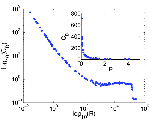
Figure 3: (Color online) Early measurements of the drag on a sphere Goldstein (1965).

Figure 3 shows the experimental data at this point, prior to the next theoretical development, matched asymptotics. Although the experimental data seem to paint a consistent portrait of the function $C_{D}(R)$, in reality they are not good enough to discriminate between different theoretical predictions.

Finite geometries cause the most significant experimental errors for these measurements Tritton (1988); Maxworthy (1965); Lindgren (1999). Tritton notes that “the container diameter must be more than one hundred times the sphere diameter for the error to be less than 2 percent”, and Lindgren estimates that a ratio of 50 between the container and sphere diameters will result in a 4% change in drag force.

In 1961, Fidleris et al. experimentally studied the effects of finite container size on drag coefficient measurements Fidleris and Whitmore (1961). They concluded that there were significant finite size effects in previous experiments, but also proposed corrections to compensate for earlier experimental limitations. Lindgren also conducted some related experiments Lindgren (1999).

T. Maxworthy also realized this problem, and undertook experiments which could be used to evaluate the more precise predictions of matched asymptotics theories. In his own words,

From the data plotted in Goldstein or Perry, it would appear that the presently available data is sufficient to accurately answer any reasonable question. However, when the data is plotted ‘correctly’; that is, the drag is non-dimensionalized with respect to the Stokes drag, startling inaccuracies appear. It is in fact impossible to be sure of the drag to better than $\pm 20\%$ … The difficulties faced by previous investigators seemed to be mainly due to an inability to accurately compensate for wall effects Maxworthy (1965).

Maxworthy refined the falling sphere technique to produce the best experimental measurements yet — $2\%$ error. He also proposed a new way of plotting the data, which removes the $R^{-1}$ divergence in Eqn. 24 (as $R\rightarrow 0$). His approach makes clear the failings of earlier measurements, as can be seen in Figure 4, where the drag measurements are normalized by the Stokes drag, $C_{D}^{\textrm{Stokes}}=6\pi/R$.

\psfrag{Re}{\mbox{\Large$R$}}\psfrag{CD}{\mbox{\Large$C_{D}R/6\pi-1$}}\psfrag{Maxworthy}{Maxworthy}\psfrag{Previous Expts.}{Previous Expts.}\includegraphics[width=346.89731pt]{fig4}

Figure 4: (Color online) Maxworthy’s accurate measurements of the drag on a sphere Maxworthy (1965) contrasted with previous experiments Goldstein (1965).

In Maxworthy’s apparatus, the container diameter is over 700 times the sphere diameter, and does not contribute significantly to experimental error, which he estimates at better than 2 percent. Note that the data in Figure 4 are digitized from his paper, as raw data are not available.

This problem also attracted the attention of atmospheric scientists, who realized its significance in cloud physics, where “cloud drops may well be approximated by rigid spheres.”Pruppacher and Le Clair (1970) In a series of papers (e.g., Pruppacher and Le Clair (1970); Pruppacher and Steinberger (1968); Beard and Pruppacher (1969); Le Clair and Hamielec (1970)), H.R. Pruppacher and others undertook numerical and experimental studies of the drag on the sphere. They were motivated by many of the same reasons as Maxworthy, because his experiments covered only Reynolds numbers between 0.4 and 11, and because “Maxworthy’s experimental setup and procedure left considerable room for improvement” Pruppacher and Steinberger (1968).

Their results included over 220 measurements, which they binned and averaged. They presented their results in the form of a set of linear fits. Adopting Maxworthy’s normalization, we collate and summarize their findings in Eqn. 27.

$$C_{D}\frac{R}{6\pi}-1=\left\{\begin{array}[]{ll}0.102\left(2R\right)^{0.955}&0.005<R\leq 1.0\\ 0.115\left(2R\right)^{0.802}&1.0<R\leq 20\\ 0.189\left(2R\right)^{0.632}&20<R\leq 200\end{array}\right.$$ (27)

Unfortunately, one of their later papers includes the following footnote (in our notation): “At $R<1$ the most recent values of $C_{D}R/6\pi-1$ (Pruppacher, 1969, unpublished) tended to be somewhat higher than those of Pruppacher and Steinberger.” Le Clair and Hamielec (1970) Their subsequent papers plot these unpublished data as “experimental scatter.” As the unpublished data are in much better agreement with both Maxworthy’s measurements and their own numerical analysis Le Clair and Hamielec (1970), it makes us question the accuracy of the results given in Eqn. 27.

There are many other numerical calculations of the drag coefficient for a sphere, including: Dennis Dennis and Walker (1971), Le Clair Le Clair and Hamielec (1970); Pruppacher and Le Clair (1970), Hamielec Hamielec et al. (1967), Rimon Rimon and Cheng (1969), Jenson Jenson (1959), and Kawaguti Kawaguti (1950). Most of these results are not useful either because of large errors (e.g., Jenson), or because they study ranges of Reynolds number which do not include $R<1$. Many numerical studies examine only a few (or even just a single) Reynolds numbers. For the purposes of comparing theoretical predictions of $C_{D}$ at low Reynolds number, only Dennis Dennis and Walker (1971) and Le Clair Le Clair and Hamielec (1970) have useful calculations. Both of these papers report tabulated results which are in very good agreement with both each other and Maxworthy; at $R=0.5$, the three sets of results agree to within 1% in $C_{D}$, and to within 10% in the transformed variable, $C_{D}R/6\pi-1$. The agreement is even better for $R<0.5$.

\psfrag{Re}{\mbox{\Large$R$}}\psfrag{CD}{\mbox{\Large$C_{D}R/6\pi-1$}}\psfrag{CD2 XXXXXXX}{\tiny{$C_{D}R/6\pi-1$}}\psfrag{Maxworthy XXXXXX}{Maxworthy}\psfrag{Pruppacher}{Eqn. \ref{Pruppacher1}}\psfrag{Le Clair}{Le Clair}\psfrag{Dennis}{Dennis}\includegraphics[width=346.89731pt]{fig5}

Figure 5: (Color online) A summary of experimental and numerical studies of $C_{D}$ for a sphere Maxworthy (1965); Le Clair and Hamielec (1970); Dennis and Walker (1971).

Figure 5 shows all relevant experimental and numerical results for the drag on a sphere. Note the clear disagreement between Pruppacher’s results (Eqn. 27), and all of the other results for $R<1$ — including Le Clair and Pruppacher’s numerical results Le Clair and Hamielec (1970). This can be clearly seen in the inset graph. Although Pruppacher’s experiment results do agree very well with other data for larger values of $R$ ($R\gtrsim 20$), we will disregard them for the purposes of evaluating theoretical predictions at low Reynolds number.

It should also be noted that there is a community of researchers interested in sedimentation and settling velocities who have studied the drag on a sphere. In a contribution to this literature, Brown reviews all of the authors discussed here, as he tabulates $C_{D}$ for $R<5000$ Brown and Lawler (2003). His report addresses a larger range of Reynolds numbers and he summarizes a number of experiments not treated here. His methodology is to apply the Fidleris’ correction Fidleris and Whitmore (1961) to previous experiments where tabulated experimental data was published. While this yields a reasonably well-behaved drag coefficient for a wide range of Reynolds numbers, it is not particularly useful for our purposes, as less accurate work obfuscates the results of the most precise experiments near $R=0$. It also does not include numerical work or important results which are only available graphically (e.g., Maxworthy Maxworthy (1965)).

II.1.2 Measuring the drag on a cylinder

Experiments designed to measure the drag on an infinite cylinder in a uniform fluid came later than those for spheres. In addition to being a more difficult experiment — theoretical calculations assume the cylinder is infinite — there were no theoretical predictions to test before Lamb’s result in 1911 Lamb H. (1911).

In 1914, E. F. Relf conducted the first experiments Relf (1914). These looked at the force exerted on long wires in a fluid. Relf measured the drag down to a Reynolds number of about ten. In 1921, Wieselberger measured the drag at still lower Reynods number, reaching $R=2.11$ by looking at the deflection of a weight suspended on a wire in an air stream Wieselsberger (1921).

These experiments, combined with others Linke (1931); Goldstein (1965) at higher Reynolds number, characterize the drag over a range of Reynolds numbers (see Goldstein, pg. 15). However, they do not probe truly small Reynolds numbers ($R\ll 1$), and are of little use for evaluating theories which are only valid in that range. Curiously, there are no shortage of claims otherwise, such as Lamb, who says “The formula is stated to be in good agreement with experiment for sufficiently small values of $U_{\infty}a/\nu$; see Wieselsberger” Lamb (1932).

In 1933, Thom measured the “pressure drag”, extending observations down to $R=1.75$. Thom also notes that this Reynolds number is still too high to compare with calculations: “Actually, Lamb’s solution only applies to values of $R$ less than those shown, in fact to values much less than unity, but evidently in most cases the experimental results are converging with them.” Thom (1933)

In 1946, White undertook a series of measurements, which were flawed due to wall effects White (1946). The first high quality experiments which measured the drag at low Reynolds number were done by R. K. Finn Finn (1953). His results, available only in graphical form, are reproduced in Figure 7. While vastly superior to any previous results, there is considerable scatter in Finn’s measurements, and they have largely been surpassed by later experiments.

Tritton, in 1959, conducted experiments which reached a Reynolds number of $R=0.2$, and also filled in some gaps in the $R-C_{D}$ curve Tritton (1959). Tritton estimates his accuracy at $\pm 6\%$, and compares his results favorably to previous work, commenting that, “Probably the lowest R points of the other workers were stretching their techniques a little beyond their limits.” Tritton is also the first author to give a discussion of systematic errors. Tritton’s results are shown in Figure 6. All of his data are available in tabular form.

\psfrag{Re}{$R=\frac{U_{\infty}a}{\nu}$}\psfrag{Log}{$\log_{10}$}\psfrag{Previous Experiments and}{Previous Expts. \cite[cite]{\@@bibref{Authors Phrase1YearPhrase2}{Goldstein38}{\@@citephrase{(}}{\@@citephrase{)}}}}\includegraphics[width=346.89731pt]{fig6}

Figure 6: (Color online) Tritton’s measurements of the drag on a cylinder Tritton (1959).

Maxworthy improved plots of the drag on a sphere (Fig. 3), by arguing that the leading divergence must be removed to better compare experiments and predictions (Fig. 4). This same criticism applies to plots of the drag on a cylinder. In the case of the cylinder, $C_{D}$ goes as $R^{-1}$ (with logarithmic corrections) as $R\rightarrow 0$ (Eqn. 19). This means we ought to plot $C_{D}R/4\pi$. This function tends to zero as $R\rightarrow 0$, so it is not necessary to plot $C_{D}R/4\pi-1$, as in the case of the sphere. Figure 7 shows both Finn’s and Tritton’s data re-plotted with the leading divergence removed.

In 1965, K. O. L. F. Jayaweera Jayaweera and Mason (1965) undertook drag measurements of the drag on very long (but finite) cylinders. At very low Reynolds number ($R\leq 0.135$), his data are available in tabular form. At higher Reynolds number, they had to be digitized. His data, plotted with the leading divergence removed, are also shown in Figure 7.

\psfrag{Re}{\mbox{\Large$R$}}\psfrag{CD}{\mbox{\Large$C_{D}R/4\pi$}}\psfrag{CD2 XXXXXXX}{\tiny{$C_{D}R/4\pi$}}\psfrag{Jayaweera XXXXX}{Jayaweera}\psfrag{Finn}{Finn}\psfrag{Tritton}{Tritton }\includegraphics[width=346.89731pt]{fig7}

Figure 7: (Color online) Summary of measurements of the drag on a cylinder Jayaweera and Mason (1965); Finn (1953); Tritton (1959).

The agreement amongst these experiments is excellent. Henceforth, Finn’s data will not be plotted, as it exhibits larger experimental variations, and is surpassed by the experiments of Jayaweera and Tritton. Jayaweera’s data exhibit the least scatter, and may be slightly better than Tritton’s. However, both experiments have comparable, large ratios of cylinder length to width (the principle source of experimental error), and there is no a priori reason to favor one experimental design over the other. We consider these two experiments to be equivalent for the purposes of evaluating theoretical predictions.

As with the sphere, there are numerical calculations, including: Underwood Underwood (1969), Son Son and Hanratty (1969), Kawaguti Kawaguti and Jain (1966), Dennis Dennis and Shmshoni (1965), Thom Thom (1933), Apelt Apelt (1961), and Allen Allen and Southwell (1955). Of these, most treat only a few Reynolds numbers, none of which are sufficiently small. Others, such as Allen and Dennis, have had their results subsequently questioned Underwood (1969). The only applicable studies are Kawaguti Kawaguti and Jain (1966), and Underwood Underwood (1969). Kawaguti has a calculation only for $R=0.5$, and is omitted. Underwood’s results are in principle important and useful, but are only available in a coarse plot, which cannot be digitized with sufficient accuracy. Consequently, no numerical results will be used for evaluating analytical predictions.

There are many different experimental and numerical drag coefficient measurements. We will subsequently use only the best as benchmarks for evaluating the performance of theoretical predictions. In the case of the sphere, the experimental measurements of Maxworthy Maxworthy (1965) as well as the numerical calculations of Dennis Dennis and Walker (1971) and Le Clair Le Clair and Hamielec (1970) all extend to sufficiently small $R$ and possess sufficient accuracy. For the cylinder the experiments of both Tritton Tritton (1959) and Jayaweera Jayaweera and Mason (1965) are both excellent. Although they exhibit small differences, we cannot judge either to be superior, and we will compare both with theoretical results.

II.2 Theoretical history

Since these problems were posed by Stokes in 1851, there have been many attempts to solve them. All of these methods involve approximations, which are not always rigorous (or even explicitly stated). There is also considerable historical confusion over contributions and attribution. Here we review and summarize the substantial contributions to the literature, focusing on what approximations are used, in both deriving governing equations and in their subsequent solution. We discuss the validity and utility of important results. Finally, we emphasize methodological shortcomings and how they have been surmounted.

II.2.1 Stokes and paradoxes

In the first paper on the subject, Stokes approximated $R=0$ in Eqn. 6 and solved the resulting equation (a problem equivalent to solving Eqn. 12 with $R=0$) Stokes (1851). After applying the boundary conditions (Eqn. 14), his solution is given in terms of a stream function by Eqn. 28.

$$\psi(r,\mu)=\frac{1}{4}\left(2r^{2}-3r+\frac{1}{r}\right)\left(1-\mu^{2}\right)$$ (28)

By substituting $\psi(r,\mu)$ into Eqns. 11, 24, and 25 (or by using Eqn. 26), we reproduce the famous result of Stokes, given by Eqn. 29.

$$C_{D}=\frac{6\pi}{R}$$ (29)

Stokes also tackled the two dimensional cylinder problem in a similar fashion, but could not obtain a solution. The reason for his failure can be seen by setting $R=0$ in Eqn. 9, and attempting a direct solution. Enforcing the $\sin\theta$ angular dependence results in a solution of the form $\psi(r,\theta)=\left(C_{1}r^{3}+C_{2}r\ln{r}+C_{3}r+C_{4}/r\right)\sin\theta$. Here $C_{i}$ are integration constants. No choice of $C_{i}$ will meet the boundary conditions Eqn. (10), as this solution cannot match the uniform flow at large $r$. The best one can do is to set $C_{1}=0$, resulting in a partial solution:

$$\psi(r,\theta)=C\left(2r\ln{r}-r+\frac{1}{r}\right)\sin\theta$$ (30)

Nonetheless, this solution is not a description of fluid flow which is valid everywhere. Moreover, due to the indeterminable constant $C$, Eqn. 30 cannot be used to estimate the drag on the cylinder.

A more elegant way to see that no solution may exist is through dimensional analysis Landau and Lifschitz (1999); Happel and Brenner (1973). The force per unit length may only depend on the cylinder radius, fluid viscosity, fluid density, and uniform stream velocity. These quantities are given in Table 3, with $M$ denoting a unit of mass, $T$ a unit of time, and $L$ a unit of length. From these quantities, one may form two dimensionless groups Buckingham (1914): $\Pi_{0}=R=|\vec{u}_{\infty}|a/\nu$, $\Pi_{1}=F_{\text{Net}}/(\rho\nu|\vec{u}_{\infty}|)$. Buckingham’s $\Pi$ Theorem Buckingham (1914) then tells us that:

$$\Pi_{0}=F(R)$$ (31)

If we make the assumption that the problem does not depend on $R$, as Stokes did, then we obtain $\Pi_{1}=\text{const}$, whence

$$F_{\text{Net}}\propto\rho\nu|\vec{u}_{\infty}|$$ (32)

However, Eqn. 32 does not depend on the cylinder radius, $a$! This is physically absurd, and demonstrates that Stokes’ assumptions cannot yield a solution. The explanation is that when we take the $R\rightarrow 0$ limit in Eqn. 31, we made the incorrect assumption that $F(R)$ tended toward a finite, non-zero limit. This is an example of incomplete similarity, or similarity of the second kind (in the Reynolds number) Barenblatt (1996). Note that the problem of flow past a sphere involves force, not force per unit length, and therefore is not subject to the same analysis.

Quantity	Description	Dimensions
$F_{\text{Net}}$	Net Force per Unit Length	$MT^{-2}$
$\nu$	Kinematic Viscosity	$L^{2}T^{-1}$
$a$	Cylinder Radius	$L$
$\rho$	Fluid Density	$ML^{-3}$
$|\vec{u}_{\infty}|$	The Uniform Stream Speed	$LT^{-1}$

Table 3: Dimensional analysis of Stokes’ problem.

Stokes incorrectly took this nonexistence of a solution to mean that steady-state flow past an infinite cylinder could not exist. This problem, which is known as Stokes’ paradox, has been shown to occur with any unbounded two-dimensional flow Krakowski and Charnes (1953). But such flows really do exist, and this mathematical problem has since been resolved by the recognition of the existence of boundary layers.

In 1888, Whitehead, attempted to find higher approximations for flow past a sphere, ones which would be valid for small but non-negligible Reynolds numbers Whitehead (1888). He used Stokes’ solution (Eqn. 28) to approximate viscous contributions (the LHS of Eqn. 12), aiming to iteratively obtain higher approximations for the inertial terms. In principle, this approach can be repeated indefinitely, always using a linear governing equation to obtain higher order approximations. Unfortunately, Whitehead found that his next order solution could not meet all of the boundary conditions (Eqn. 14), because he could not match the uniform stream at infinity Van Dyke (1975). These difficulties are analogous to the problems encountered in Stokes’ analysis of the infinite cylinder.

Whitehead’s approach is equivalent to a perturbative expansion in the Reynolds number, an approach which is “never valid in problems of uniform streaming” Proudman and Pearson (1957). This mathematical difficulty is common to all three-dimensional uniform flow problems, and is known as Whitehead’s paradox. Whitehead thought this was due to discontinuities in the flow field (a “dead-water wake”), but this is incorrect, and his “paradox” has also since been resolved Van Dyke (1975).

II.2.2 Oseen’s equation

a. Introduction

In 1893, Rayleigh pointed out that Stokes’ solution would be uniformly applicable if certain inertial forces were included, and noted that the ratio of those inertial forces to the viscous forces which Stokes considered could be used to estimate the accuracy of Stokes’ approximations Lord Rayleigh (1893).

Building on these ideas in 1910, C. W. Oseen proposed an ad hoc approximation to the Navier-Stokes equations which resolved both paradoxes. His linearized equations (the Oseen equations) attempted to deal with the fact that the equations governing Stokes’ perturbative expansion are invalid at large $|\vec{r}|$, where they neglect important inertial terms. In addition to Oseen, a number of workers have applied his equations to a wide variety of problems, including both the cylinder and the sphere.

Oseen’s governing equation arises independently in several different contexts. Oseen derived the equation in an attempt to obtain an approximate equation which describes the flow everywhere. In modern terminology, he sought a governing equation whose solution is a uniformly valid approximation to the Navier-Stokes equations. Whether he succeeded is a matter of some debate. The short answer is “Yes, he succeeded, but he got lucky.”

This story is further complicated by historical confusion. Oseen’s equations “are valid but for the wrong reason” Lindgren (1999); Oseen originally objected to working in the inertial frame where the solid body is at rest, and therefore undertook calculations in the rest frame of uniform stream. This complication is overlooked largely because many subsequent workers have only understood Oseen’s intricate three paper analysis through the lens of Lamb’s later work Lamb H. (1911). Lamb — in addition to writing in English — presents a clearer, “shorter way of arriving at his [Oseen’s] results”, which he characterizes as “somewhat long and intricate.” Lamb H. (1911)

In 1913 Fritz Noether, using both Rayleigh’s and Oseen’s ideas, analyzed the problem using stream functions Noether (1913). Noether’s paper prompted criticisms from Oseen, who then revisited his own work. A few months later, Oseen published another paper, which included a new result for $C_{D}$ (Eqn. 39) Oseen (1913). Burgess also explains the development of Oseen’s equation, and presents a clear derivation of Oseen’s principal results, particularly of Oseen’s new formula for $C_{D}$ Burgess R.W. (1916).

Lindgren offers a detailed discussion of these historical developments Lindgren (1999). However, he incorrectly reports Noether’s publication date as 1911, rather than 1913. As a result, he incorrectly concludes that Noether’s work was independent of Oseen’s, and contradicts claims made in Burgess Burgess R.W. (1916).

Although the theoretical justification for Oseen’s approximations is tenuous, its success at resolving the paradoxes of both Stokes and Whitehead led to widespread use. Oseen’s equation has been fruitfully substituted for the Navier-Stokes’ equations in a broad array of low Reynolds number problems. Happel and Brenner describe its application to many problems in the dynamics of small particles where interactions can be neglected Happel and Brenner (1973). Many workers have tried to explain the utility and unexpected accuracy of Oseen’s governing equations.

Finally, the Oseen equation, as a partial differential equation, arises in both matched asymptotic calculations and in our new work. In these cases, however, its genesis and interpretation is entirely different, and the similarity is purely formal. Due to its ubiquity and historical significance, we now discuss both Oseen’s equation and its many different solutions in detail.

b. Why Stokes’ approximation breaks down

Oseen solved the paradoxes of Stokes and Whitehead by using Rayleigh’s insight: compare the magnitude of inertial and viscous forces Oseen (1910); Lord Rayleigh (1893). Stokes and Whitehead had completely neglected inertial terms in the Navier-Stokes equations, working in the regime where the Reynolds number is insignificantly small (so-called “creeping flow”). However, this assumption can only be valid near the surface of the fixed body. It is never valid everywhere.

To explain why, we follow here the spirit of Lamb’s analysis, presenting Oseen’s conclusions “under a slightly different form.” Lamb H. (1911)

Consider first the case of the sphere. We can estimate the magnitude of the neglected inertial terms by using Stokes’ solution (Eqn. 28). Substituting this result into the RHS of Eqn. 12, we see that the dominant inertial components are convective accelerations arising from the nonlinear terms in Eqn. 12. These terms reflect interactions between the uniform stream and the perturbations described by Eqn. 28. For large values of $|\vec{r}|$, these terms are of $\mathcal{O}\left(Rr^{-2}\right)$.

Estimating the magnitude of the relevant viscous forces is somewhat trickier. If we substitute Eqn. 28 into the LHS of Eqn. 12, the LHS vanishes identically. To learn anything, we must consider the terms individually. There are two kinds of terms which arise far from the sphere. Firstly, there are components due solely to the uniform stream. These are of $\mathcal{O}\left(r^{-2}\right)$. However, the uniform stream satisfies Eqn. 12 independently, without the new contributions in Stokes’ solution. Mathematically, this means that all of the terms of $\mathcal{O}\left(r^{-2}\right)$ necessarily cancel amongst themselves. We are interested in the magnitude of the remaining terms, perturbations which result from the other components of Stokes’ solution. These viscous terms (i.e. the $\partial_{\theta}^{4}$ term in Eqn. 12) are of $\mathcal{O}\left(r^{-3}\right)$ as $r\to\infty$.

Combining these two results, the ratio of inertial to viscous terms, in the $r\to\infty$ limit, is given by Eqn. 33.

$$\frac{\textrm{inertial}}{\textrm{viscous}}=\mathcal{O}\left(Rr\right)$$ (33)

This ratio is small near the body ($r$ is small) and justifies neglecting inertial terms in that regime. However, Stokes’ implicit assumption that inertial terms are everywhere small compared to viscous terms breaks down when $Rr\sim\mathcal{O}\left(1\right)$, and the two kinds of forces are of the same magnitude. In this regime, Stokes’ solution is not valid, and therefore cannot be used to estimate the inertial terms (as Whitehead had done). Technically speaking, Stokes’ approximations breaks down because of a singularity at infinity, an indication that this is a singular perturbation in the Reynolds’ number. As Oseen pointed out, this is the genesis of Whitehead’s “paradox”.

What does this analysis tell us about the utility of Stokes’ solution? Different opinions can be found in the literature. Happel, for instance, claims that it “is not uniformly valid” Happel and Brenner (1973), while Proudman asserts “Stokes’ solution is therefore actually a uniform approximation to the total velocity distribution.” Proudman and Pearson (1957) By a uniform approximation, we mean that the approximation asymptotically approaches the exact solution as the Reynolds’ number goes to zero Kaplun and Lagerstrom (1957); see Section II.3 for further discussion.

Proudman and Pearson clarify their comment by noting that although Stokes’ solution is a uniform approximation to the total velocity distribution, it does not adequately characterize the perturbation to the uniform stream, or the derivatives of the velocity. This is a salient point, for the calculations leading to Eqn. 33 examine components of the Navier-Stokes equations, not the velocity field itself. These components are forces — derivatives of velocity.

However, Proudman and Pearson offer no proof that Stokes’ solution is actually a uniform approximation, and their claim that it is “a valid approximation to many bulk properties of the flow, such as the resistance” Proudman and Pearson (1957) goes unsupported. In fact any calculation of the drag necessitates utilizing derivatives of the velocity field, so their argument is inconsistent.

We are forced to conclude that Stokes’ solution is not a uniformly valid approximation, and that his celebrated result, Eqn. 29, is the fortuitous result of uncontrolled approximations. Remarkably, Stokes’ drag formula is in fact the correct zeroth order approximation, as can be shown using either matched asymptotics or the Oseen equation! This coincidence is essentially due to the fact that the drag is determined by the velocity field and its derivatives at the surface of the sphere, where $r=1$, and Eqn. 33 is $\mathcal{O}\left(R^{1}\right)$. The drag coefficient calculation uses Stokes’ solution in the regime where his assumptions are the most valid.

A similar analysis affords insight into the origin of Stokes’ paradox in the problem of the cylinder. Although we have seen previously that Stokes’ approach must fail for both algebraic and dimensional considerations, examining the ratio between inertial and viscous forces highlights the physical inconsistencies in his assumptions.

We can use the incomplete solution given by Eqn. 30 to estimate the relative contributions of inertial and viscous forces in Eqn. 9. More specifically, we examine the behavior of these forces at large values of $r$. Substituting Eqn. 30 into the RHS of Eqn. 9, we find that the inertial forces are $\mathcal{O}\left(RC^{2}\log{r}/{r^{2}}\right)$ as $r\rightarrow\infty$.

We estimate the viscous forces as in the case of the sphere, again ignoring contributions due solely to the uniform stream. The result is that the viscous forces are $\mathcal{O}\left(C\log{r}/{r^{3}}\right)$. Combining the two estimates, we obtain the result given in Eqn. 34.

$$\frac{\textrm{inertial}}{\textrm{viscous}}=\mathcal{O}\left(Rr\right)$$ (34)

This result demonstrates that the paradoxes of Stokes and Whitehead are the result of the same failures in Stokes’ uncontrolled approximation. Far from the solid body, there is a regime where it is incorrect to assume that the inertial terms are negligible in comparison to viscous terms. Although these approximations happened to lead to a solution in the case of the sphere, Stokes’ approach is invalid and technically inconsistent in both problems.

c. How Oseen Resolved the Paradoxes

Not only did Oseen identify the physical origin for the breakdowns in previous approximations, but he also discovered a solution Oseen (1910). As explained above, the problems arise far from the solid body, when inertial terms are no longer negligible. However, in this region ($r\gg 1$), the flow field is nearly a uniform stream — it is almost unperturbed by the solid body. Oseen’s inspiration was to replace the inertial terms with linearized approximations far from the body. Mathematically, the fluid velocity $\vec{u}$ in Eqn. 6 is replaced by the quantity $\vec{u}_{\infty}+\vec{u}$, where $\vec{u}$ represents the perturbation to the uniform stream, and is considered to be small. Neglecting terms of $\mathcal{O}\left(|\vec{u}|^{2}\right)$, the viscous forces of the Navier-Stokes’ equation — $R\left(\vec{u}\cdot\nabla\vec{u}\right)$ — are approximated by $R\left(\vec{u}_{\infty}\cdot\nabla\vec{u}\right)$.

This results in Oseen’s equation:

$$R\left(\vec{u}_{\infty}\cdot\nabla\vec{u}\right)=-\nabla p+\nabla^{2}\vec{u}$$ (35)

The lefthand side of this equation is negligible in the region where Stokes’ solution applies. One way to see this is by explicitly substituting Eqn. 28 or Eqn. 30 into the LHS of Eqn. 35. The result is of $\mathcal{O}\left(R\right)$. This can also be done self-consistently with any of the solutions of Eqn. 35; it can thereby be explicitly shown that the LHS can only becomes important when $r\gg 1$, and the ratios in Eqns. 33 and 34 are of $\mathcal{O}\left(1\right)$.

Coupled with the continuity equation (Eqn. 5), and the usual boundary conditions, the Oseen equation determines the flow field everywhere. The beautiful thing about Oseen’s equation is that it is linear, and consequently is solvable in a wide range of geometries. In terms of stream functions, the Oseen equation for a sphere takes on the form given by Eqn. 36. The boundary conditions for this equation are still given by Eqn. 14.

$$D^{4}\psi=R\left(\frac{1-\mu^{2}}{r}\frac{\partial}{\partial\mu}+\mu\frac{\partial}{\partial r}\right)D^{2}\psi(r,\mu)$$ (36)

Here, $D$ is defined as in Eqn. 12.

For the cylinder, where the boundary conditions are given by Eqn. 10, Oseen’s equation takes the form given by Eqn. 37.

$$\nabla_{r}^{4}\psi(r,\theta)=R\left(\cos(\theta)\frac{\partial}{\partial r}-\frac{\sin(\theta)}{r}\frac{\partial}{\partial\theta}\right)\nabla_{r}^{2}\psi(r,\theta)$$ (37)

Here $\nabla$ is defined as in Eqn. 9. This equation takes on a particularly simple form in Cartesian coordinates (where $x=r\cos{\theta}$): $\left(\nabla^{2}-R\partial_{x}\right)\nabla^{2}\psi(r,\theta)=0$.

A few historical remarks must be made. First, Oseen and Noether were motivated to refine Stokes’ work and include inertial terms because they objected to the analysis being done in the rest frame of the solid body. While their conclusions are valid, there is nothing wrong with solving the problem in any inertial frame. Secondly, Oseen made no use of stream functions; the above equations summarize results from several workers, particularly Lamb.

There are many solutions to Oseen’s equations, applying to different geometries and configurations, including some exact solutions. However, for any useful calculations, such as $C_{D}$, even the exact solutions need to be compromised with approximations. There have been many years of discussion about how to properly interpret Oseen’s approximations, and how to understand the limitations of both his approach and concomitant solutions. Before embarking on this analysis, we summarize the important solutions to Eqns. 36 and 37.

d. A plethora of solutions

Oseen himself provided the first solution to Eqn. 36, solving it exactly for flow past a sphere Oseen (1910). Eqn. 38 reproduces this result in terms of stream functions, a formula first given by Lamb Lamb (1932).

$$\psi(r,\theta)=\frac{1}{4}\left(2r^{2}+\frac{1}{r}\right)\sin^{2}{\theta}-\frac{3}{2R}\left(1+\cos{\theta}\right)\left(1-e^{-\frac{1}{2}Rr\left(1-\cos{\theta}\right)}\right)$$ (38)

This solution is reasonably behaved everywhere, and may be used to obtain Oseen’s improved approximation for the drag coefficient (Eqn. 39).

$$C_{D}=\frac{6\pi}{R}\left(1+\frac{3}{8}R\right)+\mathcal{O}\left(R^{2}\right)$$ (39)

Oseen obtained this prediction for $C_{D}$ after the prompting of Noether, and only presented it in a later paper Oseen (1913). Burgess also obtained this result Burgess R.W. (1916). Oseen’s work was hailed as a resolution to Whitehead’s paradox. While it did resolve the paradoxes (e.g., he explained how to deal with inertial terms), and his solution is uniformly valid, it does not posses sufficient accuracy to justify the “$3/8R$” term in Eqn. 39. What Oseen really did was to rigorously derive the leading order term, proving the validity of Stokes’ result (Eqn. 29). Remarkably, his new term is also correct! This is a coincidence which will be carefully considered later.

This solution (Eqn. 38) is exact in the sense that it satisfies Eqn. 36. However, it does not exactly meet the boundary conditions (Eqn. 14) at the surface of the sphere. It satisfies those requirements only approximately, to $\mathcal{O}\left(R^{1}\right)$. This can readily be seen by expanding Eqn. 38 about $r=1$:

$$\psi(r,\theta)=\frac{1}{4}\left(2r^{2}-3r+\frac{1}{r}\right)\sin^{2}{\theta}+\mathcal{O}\left(R^{1}\right)$$ (40)

Up to $\mathcal{O}\left(R\right)$ this is simply Stokes’ solution (Eqn. 28), which vanishes identically at $r=1$. The new terms fail to satisfy the boundary conditions at the surface, but are higher order in $R$. Thus Oseen’s solution is an exact solution to an approximate governing equation which satisfies boundary conditions approximately. The implications of this confounding hierarchy of approximations will be discussed below.

Lamb contributed a simplified method for both deriving and solving Oseen’s equation Lamb H. (1911). His formulation was fruitfully used by later workers (e.g., Faxén (1927); Goldstein (1929); Tomotika and Aoi (1950)), and Lamb himself used it both to reproduce Oseen’s results and to obtain the first result for the drag on an infinite cylinder.

Lamb’s basic solution for flow around an infinite cylinder appears in a number of guises. His original solution was given in terms of velocity components, and relied on expansions of modified Bessel functions which kept only the most important terms in the series. This truncation results in a solution (Eqn. 41) which only approximately satisfies the governing equations (Eqn. 37), and is only valid near the surface.

$$u_{x} = 1+\delta\left(\gamma-\frac{1}{2}+\log{\frac{rR}{4}}+\frac{1}{2}\left(r^{2}-1\right)\frac{\partial^{2}}{\partial x^{2}}\log{r}\right)$$ (41a)

$$u_{y} = \frac{\delta}{2}\left(r^{2}-1\right)\frac{\partial^{2}}{\partial x\partial y}\log{r}$$ (41b)

$$u_{z} = 0$$ (41c)

In this equation, $\delta=\left(\frac{1}{2}-\gamma-\log{\frac{R}{4}}\right)^{-1}$.

Note that, although it only approximately satisfies Oseen’s governing equation, this result satisfies the boundary conditions (Eqn. 4) exactly. Lamb used his solution to derive the first result (Eqn. 42) for the drag on an infinite cylinder, ending Stokes’ paradox:

$$C_{D}=\frac{4\pi}{R}\left(\delta\right)$$ (42)

In his own words, “ … Stokes was led to the conclusion that steady motion is impossible. It will appear that when the inertia terms are partially taken into account … that a definite value for the resistance is obtained.” Lamb H. (1911) As with all analysis based on the ad-hoc Oseen equation, it is difficult to quantify either the accuracy or the limitations of Lamb’s result.

Many authors formulate alternate expressions of Lamb’s solution by retaining the modified Bessel functions rather than replacing them with expansions valid for small $R$ and $r$. This form is given by Eqn. 43, and is related to the incomplete form given by VanDyke (p. 162) Van Dyke (1975).

$$u_{x} = 1+\delta\left(\frac{x^{2}}{r^{4}}-\frac{1}{2r^{2}}+\frac{2x}{Rr^{2}}-e^{Rx/2}K_{0}\left(\frac{Rr}{2}\right)-\frac{x}{r}e^{Rx/2}K_{1}\left(\frac{Rr}{2}\right)\right)$$ (43a)

$$u_{y} = \delta\left(\frac{xy}{r^{4}}+\frac{2y}{Rr^{2}}-\frac{y}{r}e^{Rx/2}K_{1}\left(\frac{Rr}{2}\right)\right)$$ (43b)

$$u_{z} = 0$$ (43c)

Here $I_{n}$ and $K_{n}$ are modified Bessel functions.

In contrast to Eqn. 41, this solution is an exact solution to Oseen’s equation (Eqn. 37), but only meets the boundary conditions to first approximation. In particular, it breaks down for harmonics other than $\sin{\theta}$. Whether Eqn. 41 or Eqn. 43 is preferred is a matter of some debate, and ultimately depends on the problem one is trying to solve.

Some workers prefer expressions like Eqn. 43, which are written in terms of $\vec{u}$. Unlike the solutions for the stream function, these results can be written in closed form. This motivation is somewhat misguided, as applying the boundary conditions nonetheless requires a series expansion.

In terms of stream functions Eqn. 43 transforms into Eqn. 44 Proudman and Pearson (1957).

$$\psi(r,\theta)=\left(r+\frac{\delta}{2r}\right)\sin{\theta}-\sum_{n=1}^{\infty}\delta\phi_{n}\left(\frac{Rr}{2}\right)\frac{r\sin{n\theta}}{n}$$ (44)

Here,

$$\phi_{n}(x)=2K_{1}(x)I_{n}(x)+K_{0}(x)\left(I_{n+1}(x)+I_{n-1}(x)\right)$$

This result is most easily derived as a special case of Tomotika’s general solution (Eqn. 49) Tomotika and Aoi (1950), although Proudman et al. intimate that it can also be directly derived from Lamb’s solution (Eqn. 43) Proudman and Pearson (1957).

Bairstow et al. were the first to retain Bessel functions while solving Oseen’s Eqn. for flow past a cylinder Bairstow and Cave B.M. (1923). They followed Lamb’s approach, but endeavored to extend it to larger Reynolds’ numbers, and obtained the drag coefficient given in Eqn. 45. When expanded near $R=0$, this solution reproduces Lamb’s result for $C_{D}$ (Eqn. 42). It can also be obtained from Tomotika’s more general solution (Eqn. 49).

$$C_{D}=\frac{4\pi}{R\left(I_{0}(R/2)K_{0}(R/2)+I_{1}(R/2)K_{1}(R/2)\right)}$$ (45)

Bairstow also made extensive comparisons between experimental measurements of $C_{D}$ and theoretical predictions Relf (1914). He concluded, “For the moment it would appear that the maximum use has been made of Oseen’s approximation to the equations of viscous fluid motion.”

At this point, the “paradoxes” were “resolved” but by an approximate governing equation which had been solved approximately. This unsatisfactory state of affairs was summarized by Lamb in the last edition of his book: “ … even if we accept the equations as adequate the boundary-conditions have only been approximately satisfied.” Lamb (1932) His comment was prompted largely by the work of Hilding Faxén, who initiated the next theoretical development, exact solutions to Oseen’s approximate governing equation (Eqn. 35) which also exactly satisfy the boundary conditions.

Beginning with his thesis and spanning a number of papers Faxén systematically investigated the application of boundary conditions to solutions of Oseen’s equations Faxén (1923, 1921). Faxén initially studied low Reynolds number flow around a sphere, and he began by re-examining Oseen’s analysis. He derived a formula for $C_{D}$ which differed from Oseen’s accepted result (Eqn. 39). Faxén realized that this was due to differences in the application of approximate boundary conditions; within the limitations of their respective analyses, the results actually agreed.

Faxén next solved Oseen’s equation (Eqn. 36), but in bounded, finite spaces where the boundary conditions could be satisfied exactly. He initially studied flow near infinite parallel planes, but ultimately focused on flow around a sphere within a cylinder of finite radius. He aimed to calculate the drag force in a finite geometry, and then take the limit of that solution as the radius of the cylinder tends to infinity.

Unfortunately, in the low Reynolds number limit, the problem involves incomplete similarity, and it is incorrect to assume that solutions will be well behaved (e.g., tend to a finite value) as the boundary conditions are moved to infinity.

The drag force which Faxén calculated involved a number of undetermined coefficients, so he also calculated it using solutions to Stokes’ governing equations. This solution also has unknown coefficients, which he then calculated numerically. Arguing that the two solutions ought to be the same, he matched coefficients between the two results, substituted the numerical coefficients, and thereby arrived at a drag force based on the Oseen governing equation.

This work is noteworthy for two reasons. First, the matching of coefficients between solutions derived from the two different governing equations is prescient, foreshadowing the development of matched asymptotics 30 years later. Secondly, Faxén ultimately concluded that Oseen’s “improvement” (Eqn. 39) on Stokes’ drag coefficient (Eqn. 29) is invalid Faxén (1923). Faxén’s analysis demonstrates that — when properly solved — Oseen’s equation yields the same drag coefficient as Stokes’, without any additional terms Lindgren (1999).

Studies by Bohlin and Haberman concur with Faxén’s conclusions Bohlin (1960); Haberman and Saure (1958); Lindgren (1999). It is not surprising that his results reject Oseen’s new term ($3R/8$). We previously explained that Oseen’s analysis, although it eliminates the “paradoxes”, does not posses sufficient accuracy to justify more than the lowest order term in Eqn. 39.

However, Faxén’s results suffer from problems. First, they cannot be systematically used to obtain better approximations. Secondly, Faxén actually solves the problem for bounded flow, with the boundary conditions prescribed by finite geometries. He uses a limiting procedure to extend his solutions to unbounded flow (with boundary conditions imposed on the uniform stream only at infinity, as in Eqn. 4). In problems like this, which involve incomplete similarity, it is preferable to work directly in the infinite domain.

Faxén’s meticulous devotion to properly applying boundary conditions culminated in the first complete solution to Eqn. 37. In 1927, he published a general solution for flow around an infinite cylinder which could exactly satisfy arbitrary boundary conditions Faxén (1927). Unfortunately, Faxén’s solution contains an infinite number of undetermined integration constants, and approximations must be used to determine these constants. Although this destroys the “exact” nature of the solution, these approximations can be made in a controlled, systematic fashion — an improvement over the earlier results of Lamb and Oseen. Although Faxén’s heroic solution was the first of its kind, his real insight was realizing that approximations in the application of boundary conditions could be as important as the approximations in the governing equations.

His formal solutions are in essence a difficult extension of Lamb’s reformulation of Oseen’s equations, and they inspired several similar solutions. In 1929, Goldstein completed a similarly herculean calculation to derive a general solution to Oseen’s equation for flow around a sphere Goldstein (1929). Like Faxén’s result for the cylinder, Goldstein’s solution can — in principle — exactly satisfy the boundary conditions. Unfortunately, it also suffers from the same problems: It is impossible to determine all of the infinitely many integration constants.

Goldstein’s solution is summarized by Tomotika, who also translated it into the language of stream functions Tomotika and Aoi (1950). We combine elements from both papers in quoting the solution given in Eqn. 46.

$$\psi(r,\theta)=-r^{2}Q_{1}(\cos{\theta})+\sum_{n=1}^{\infty}\left(B_{n}r^{-n}+\sum_{m=0}^{\infty}X_{m}r^{2}\Phi_{m,n}(rR/2)\right)Q_{n}(\cos{\theta})$$ (46)

In this equation,

$$Q_{n}(\mu) = \int_{-1}^{\mu}P_{n}(\mu)\textrm{d}\mu$$ (47a)

$$\Phi_{m,n}(x) = -\left(\frac{m}{2m-1}\chi_{m-1}(x)+\frac{m+1}{2m+3}\chi_{m+1}(x)\right)f_{m,n}(x)$$ (47b)

$$-\left(\frac{m}{2m+1}f_{m-1,n}(x)+\frac{m+1}{2m+1}f_{m+1,n}(x)\right)\chi_{m}(x)$$

$$\chi_{m}(x) = \left(2m+1\right)\left(\frac{\pi}{2x}\right)^{\left(\frac{1}{2}\right)}K_{m+\frac{1}{2}}(x)$$ (47c)

$$f_{m,n}(x) = (2n+1)\sum_{j=0}^{m}\frac{(2j)!(2m-2j)!(2n-2j)!}{(j!)^{2}(2m+2n-2j+1)!}$$ (47d)

$$\times\left(\frac{(m+n-j)!}{(m-j)!(n-j)!}\right)^{2}\phi_{m+n-2j}(x)$$

$$\phi_{n}(x) = (2n+1)\left(\frac{\pi}{2x}\right)^{\frac{1}{2}}I_{n+\frac{1}{2}}(x)$$

$$f_{m,n}(x) = \sum_{j=0}^{m}C_{m}(k)\frac{\partial^{j}\phi_{n}(x)}{\partial x^{j}}$$ (47e)

Here $K_{n}(x)$ and $I_{n}(x)$ are Bessel functions, $P_{m}(x)$ are Legendre polynomials, and $C_{m}(k)$ is the coefficient of $x^{k}$ in $P_{m}(x)$. Note that the second expression for $f_{m,n}(x)$, written in terms of derivatives, is computationally convenient Goldstein (1929).

Eqn. 46 is given with undetermined constants of integration, $B_{n}$ and $X_{m}$. Methods to determine these constants were discussed by both Tomotika Tomotika and Aoi (1950) and Goldstein Goldstein (1929). We will present our own analysis later.

There are many different results which have been obtained using the above general solution. The exact formula for the stream function and the drag coefficient depend on what terms in the solution are retained, and how one meets the boundary conditions. In general, retaining $n$ angular terms in Eqn. 46 requires the retention of $m=n-1$ terms in the second sum. In his original paper, Goldstein retains three terms in each series, and thereby calculates the formula for $C_{D}$ given in Eqn. 48.

$$C_{D}=\frac{6\pi}{R}\left(1+\frac{3}{8}R-\frac{19}{320}R^{2}+\frac{71}{2560}R^{3}-\frac{30179}{2150400}R^{4}+\frac{122519}{17203200}R^{5}+\mathcal{O}\left(R^{6}\right)\right)$$ (48)

The coefficient of the last term reflects a correction due to Shanks Shanks (1955).

To obtain the result in Eqn. 48, Goldstein both truncated his solution for the stream function and then expanded the resulting $C_{D}$ about $R=0$. Van Dyke extended this result to include an additional 24 terms, for purposes of studying the mathematical structure of the series, but not because of any intrinsic physical meaning Van Dyke (1970). Van Dyke does not state whether he was including more harmonics in the stream function solution or simply increasing the length of the power series given in Eqn. 48.

In addition to expressing Goldstein’s solution for the geometry of a sphere in terms of stream functions, Tomotika derived his own exact solution to Eqn. 37 for flow past a cylinder Tomotika and Aoi (1950). Tomotika closely followed the spirit of Lamb Lamb H. (1911) and Goldstein Goldstein (1929), and his resulting “analysis is quite different from Faxén’s.” Tomotika and Aoi (1950). His solution to Eqn. 37 is given in Eqn. 49 below, conveniently expressed in terms of stream functions. Note that Tomotika’s result suffers from the same problems as his predecessors: An infinite number of undetermined integration constants.

$$\psi(r,\theta)=r\sin{\theta}+\sum_{n=1}^{\infty}\left(B_{n}r^{-n}+\sum_{m=0}^{\infty}X_{m}r\Phi_{m,n}(rR/2)\right)\sin{n\theta}$$ (49)

Where

$$\Phi_{m,n}(x) = \left(K_{m+1}(x)+K_{m-1}(x)\right)\left(I_{m-n}(x)+I_{m+n}(x)\right)$$ (50)

$$+K_{m}(x)\left(I_{m-n-1}(x)-I_{m-n+1}(x)-I_{m+n-1}(x)+I_{m+n+1}(x)\right)$$

As before, $B_{n}$ and $X_{m}$ are constants of integration which need to be determined by the boundary conditions (Eqn. 10).

As with Goldstein’s solution for the sphere, approximations are necessary in order to actually calculate a drag coefficient. By retaining the $m=0$ and $n=1$ terms, Tomotika reproduced Bairstow’s result for $C_{D}$ (Eqn. 45). He also numerically calculated drag coefficients based on retaining more terms. As with the Goldstein solution, keeping $n$ angular terms requires keeping $m=n-1$ terms in the second sum.

The solutions given in Eqns. 46 and 49 represent the culmination of years of efforts to solve Oseen’s equation for both the sphere and the cylinder. These general solutions are also needed in both matched asymptotics and the new techniques presented in this section Proudman and Pearson (1957).

There is a final noteworthy solution to Eqn. 37. In 1954, Imai published a general method for solving the problem of flow past an arbitrary cylindrical body Imai Isao (1954). His elegant technique, based on analytic functions, applies to more general geometries. Imai calculated a formula for $C_{D}$, approximating the functions in his exact solution with power series about $R=0$. His result (re-expressed in our notation) is given in Eqn. 51.

$$C_{D}=\frac{4\pi}{R}\delta+R\left(-\frac{\pi}{2}+\frac{\pi\delta}{4}-\frac{5\pi\delta^{2}}{32}\right)$$ (51)

Note that Imai’s result agrees with Eqn. 42 at lowest order, the only order to which Oseen’s equation really applies. A priori, his result is neither better nor worse than any other solution of Oseen’s equation. It is simply different.

e. Discussion

We have presented Oseen’s governing equations for low Reynold number fluid flow. These equations are a linearized approximation to the Navier-Stokes’ equations. We have also presented a number of different solutions, for both stream functions and drag coefficients; each of these solutions comes from a unique set of approximations. The approximations which have been made can be put into the following broad categories:

• The governing equation — Oseen’s equation approximates the Navier-Stokes equations.

• Solutions which only satisfy the Oseen’s equation approximately.

• Solutions which only satisfy the boundary conditions approximately.

• Solutions where the stream function is expanded in a power series about $R=0$ after its derivation.

• Approximations in the drag coefficient derivation.

• Drag coefficients which were expanded in a power series about $R=0$ after their derivation.

The first approximation is in the governing equations. Oseen’s approximation is an ad hoc approximation which, although it can be shown to be self-consistent, requires unusual cleverness to obtain. Because it is not derived systematically, it can be difficult to understand either its applicability or the limitations of its solutions. There have been years of discussion and confusion about both the equation and its solutions. The short answer is this: Oseen’s governing equation is a zeroth order uniformly valid approximation to the Navier Stokes equation; the equation and its solutions are valid only at $\mathcal{O}\left(R^{0}\right)$.

It is not easy to prove this claim rigorously Faxén (1923). However, it can be easily shown that Oseen’s equations are self-consistent with its solutions, and that the error in the solution is of $\mathcal{O}\left(R^{1}\right)$. One way to explicitly demonstrate this is by substituting a solution of Oseen’s equation into the LHS of the Navier-Stokes equations (Eqn. 6), thereby estimating the contribution of inertial terms for the flow field characterized by the solution. By repeating that substitution into the LHS of Oseen’s equation (Eqn. 35), one can estimate the contribution of inertial terms under Oseen’s approximations. Comparing the two results gives an estimate of the inaccuracies in Oseen’s governing equations.

Concretely, for the sphere, we substitute Eqn. 38 into the RHS of Eqn. 36, and into the RHS of Eqn. 12. The difference between the two results is of $\mathcal{O}\left(R^{1}\right)$.

For the cylinder, substitute Eqn. 44 into the RHS of Eqns. 37 and 9. The difference between the exact and approximate inertial terms is of $\mathcal{O}\left(R\delta\right)$, where $\delta$ is defined as in Eqn. 44.

These conclusions do not depend on the choice of solution (or on the number of terms retained in Eqn. 44). They explicitly show that the governing equation is only valid to $\mathcal{O}\left(R\right)$ (or $\mathcal{O}\left(R\delta\right)$). Consequently, the solutions can only be meaningful to the same order, and the boundary conditions need only be satisfied to that order. With these considerations, almost all of the solutions in the preceding section are equivalent. The only ones which are not — such as Eqn. 41 — are those in which the solution itself has been further approximated.

Since the formulae for determining $C_{D}$ (Eqns. 19 and 24) are of the form $1/R$ + terms linear in stream function + nonlinear terms, a stream function which is valid to $\mathcal{O}\left(R\right)$ will result in a drag coefficient which is valid to $\mathcal{O}\left(R^{0}\right)$. Thus, in all of the formula for $C_{D}$ which have been presented so far, only the first term is meaningful. For a sphere, this is the Stokes’ drag (Eqn. 29), and for the cylinder, Lamb’s results (Eqn. 42).

We have concluded that it is only good fortune that Oseen’s new “$3/8R$” term is actually correct. This concurs with the analysis of Proudman et al., who wrote, “Strictly, Oseen’s method gives only the leading term … and is scarcely to be counted as superior to Stokes’s method for the purpose of obtaining the drag.” Proudman and Pearson (1957) Proudman and Pearson also note that the vast effort expended finding exact solutions to Oseen’s equation is “of limited value.” Goldstein’s formula for $C_{D}$, for instance, is expanded to $\mathcal{O}\left(R^{5}\right)$, well beyond the accuracy of the original governing equations. The reason for Oseen’s good fortune is rooted in the symmetry of the problem. Chester and Van Dyke both observe that the non-linear terms which Oseen’s calculation neglects, while needed for a correct stream function, do not contribute to the drag because of symmetry Chester (1962); Van Dyke (1975).

Lindgren argues that Faxén proved that, when the boundary conditions are met properly and Oseen’s equations solved exactly, the resulting $C_{D}$ is that obtained by Stokes (Eqn. 29) Lindgren (1999). Whether this argument is correct does not matter, as Oseen’s additional term is beyond the accuracy of his governing equations.

There is another approximation which arises while computing $C_{D}$ in the context of Oseen’s equation. Many workers (e.g., Tomotika and Aoi (1950)) compute the pressure in Eqns. 19 and 24 by integrating Oseen’s equation (Eqn. 35, rather than the Navier-Stokes equations (Eqn. 6). In Eqns. 20 and 25, we presented a pressure calculation based on the Navier Stokes equations. Calculating pressure using the linearized Oseen equation introduces an additional approximation into $C_{D}$. While not necessarily problematic or inconsistent, this approximation can be difficult to identify.

f. Two different interpretations One criticism of the Oseen equation is that it may be obtained by linearizing the Navier-Stokes equations, without regard to the magnitude of inertial and viscous terms. By writing $\vec{u}=\vec{U}_{\infty}+\delta\vec{u}$, treating $\delta\vec{u}$ as a small perturbation, and expanding Eqn. 6 one can formally reproduce Oseen’s equations. Clearly, the disturbance to the uniform stream is not negligible near the surface of the solid body, and therefore Oseen’s equations “would appear to be a poor approximation in the neighborhood of the body where the boundary condition $\vec{u}=0$ requires that the true inertial term be small.” Happel and Brenner (1973)

This incorrect argument, put forth as a reason to use Stokes’ solutions, overlooks the origins of Oseen’s equations. The point of Oseen’s approximation is that inertial terms are only significant at large values of $|r|$, where $R|r|$ is no longer negligible. Near the surface of the solid, the approximate inertial terms which Oseen introduced are negligible in comparison to the viscous terms, because they are multiplied by the factor $R$ (in the LHS of Eqn. 35). Hence the difference between Oseen’s and Stokes’ equations in the neighborhood of the sphere will be of $\mathcal{O}\left(R\right)$, and is beyond the scope of either theory.

g. Better approximations

The approach of Whitehead was essentially to improve Stokes’ solution for the sphere in an iterative fashion Whitehead (1888). By substituting the first approximation into the governing equations, he estimated the neglected terms. He then tried, and failed, to solve the resulting governing equation. This approach fails because the Stokes’ equations are not uniformly valid to zeroth order.

Oseen’s equations are uniformly valid, and, as Proudman remarked, “there seems little reason to doubt that Whitehead’s iterative method, using Oseen’s equation rather than Stokes’s equation would yield an expansion, each successive term of which would represent a uniformly valid higher approximation to the flow. In each step of the iteration, a lower-order approximation would be used to calculate those particular inertia terms that are neglected … the expansion generated in this way would seem to be the most economic expansion possible.” Proudman and Pearson (1957)

Proudman did not follow through on this idea, instead developing a solution based on matched asymptotics expansions (see below). In an appendix, Van Dyke relates the unpublished work of C. R. Illingworth (1947) Van Dyke (1975). Illingworth carried through Whitehead’s program, deriving a new expression (Eqn. 52) for $C_{D}$, which agrees to $\mathcal{O}\left(R^{2}\ln{R}\right)$ with the later results of matched asymptotic calculations (Eqn. 55).

$$C_{D}=\frac{6\pi}{R}\left(1+\frac{3}{8}R+\frac{9}{40}R^{2}\log{R}+0.1333R^{2}+\frac{81}{320}R^{3}\log{R}-0.0034R^{3}+\ldots\right)$$ (52)

Although this result has since been subsumed by matched asymptotics, it is nonetheless remarkable, substantially improving any previous drag calculations, and rigorously justifying Oseen’s $3/8R$ term.

There have also been efforts (e.g., Shanks (1955); Van Dyke (1970)) to “re-sum” Goldstein’s series expansion for $C_{D}$ (Eqn. 48). However, these results have little intrinsic (as opposed to methodological) value, as Goldstein’s result is only valid to $\mathcal{O}\left(R\right)$. If applied to more accurate approximations, such as Eqn. 52, these methods could be worthwhile. Alas, even improved approximations lack a sufficient numbers of terms in the expression for $C_{D}$ to make this practicable.

h. Summary

Simply put, Oseen’s equations resolved the paradoxes of Stokes and Whitehead, put Stokes’ results on firm theoretical ground, and led to the first solution for the drag on a cylinder. Although the Oseen equations happen to provide a uniformly valid first approximation, it is difficult to extend this work to higher order approximations.

Figure 8 compares the “predictions” of Oseen theory to experimental and numerical data for the drag on a sphere. Again, Oseen’s first order theory is, strictly speaking, not adequate to make the predictions with which it is traditionally credited. The theoretical drag coefficients are roughly valid for $R\lesssim 0.2$, with Goldstein’s solution (Eqn. 48) being slightly better than Oseen’s prediction (Eqn. 39). All are clearly superior to Stokes’ formula (Eqn. 29).

Figure 8 also shows the prediction of Illingworth’s second order Oseen theory (Eqn. 52). Not surprisingly, it gives the best prediction of $C_{D}$, particularly when compared to Dennis’ numerical results.

\psfrag{Re}{\mbox{\Large$R$}}\psfrag{CD}{\mbox{\Large$C_{D}R/6\pi-1$}}\psfrag{CD2 XXXXXXX}{\tiny{$C_{D}R/6\pi-1$}}\psfrag{Maxworthy XXXXXX}{Maxworthy}\psfrag{Pruppacher}{Eqn. \ref{Pruppacher1}}\psfrag{Le Clair}{Le Clair}\psfrag{Dennis}{Dennis}\psfrag{Stokes}{Stokes, Eqn. \ref{stokes:famoussol}}\psfrag{Oseen}{Oseen, Eqn. \ref{Oseen:dragsphere}}\psfrag{Goldstein}{Goldstein, Eqn. \ref{GoldsteinCD}}\psfrag{Illingworth}{Illing., Eqn. \ref{illingworth}}\includegraphics[width=346.89731pt]{fig8}

Figure 8: (Color online) Drag on a sphere, experiment vs. Oseen theory Maxworthy (1965); Le Clair and Hamielec (1970); Dennis and Walker (1971). The Stokes’ solution (Eqn. 29) is shown at the bottom for reference. In these coordinates, it is defined by the line $y=0$.

\psfrag{Re}{\mbox{\Large$R$}}\psfrag{CD}{\mbox{\Large$C_{D}R/4\pi$}}\psfrag{Jayaweera XXXXXX}{Jayaweera}\psfrag{Tritton}{Tritton}\psfrag{Imai}{Imai, Eqn. \ref{imaisol}}\psfrag{Bairstow}{Bairstow, Eqn. \ref{Bairstowsol}}\psfrag{Lamb}{Lamb, Eqn. \ref{Oseen:LambDrag}}\includegraphics[width=346.89731pt]{fig9}

Figure 9: (Color online) Drag on a cylinder, experiment vs. Oseen theory Jayaweera and Mason (1965); Tritton (1959).

Figure 9 shows the important predictions of Oseen theory for the drag on an infinite cylinder. As with the sphere, the theory is only truly entitled to predict the lowest order term. Figure 9 shows decent agreement with the data. Although more “exact” solutions (such as Bairstow’s and Imai’s) do better than Lamb’s lowest order solution, this is purely coincidental. Tomotika’s solutions exhibit similar characteristics to these two solutions.

II.2.3 Matched asymptotics

Efforts to systematically improve Oseen’s results led to the development of matched asymptotic expansions. This branch of applied mathematics was developed gradually, with systematic work beginning with papers by Kaplun and Lagerstrom et al. Lagerstrom and Cole (1955); Kaplun (1954). Kaplun subsequently used these techniques to calculate the drag on a cylinder, obtaining an entirely new result for $C_{D}$ Lagerstrom et al. (1967). Proudman and Pearson subsequently applied matched asymptotics to both the sphere and the cylinder, deriving a new result for the drag on a sphere Proudman and Pearson (1957).

“The principle of asymptotic matching is simple. The interval on which a boundary-value problem is posed is broken into a sequence of two or more overlapping subintervals. Then, on each subinterval perturbation theory is used to obtain an asymptotic approximation to the solution of the differential equation valid on that interval. Finally, the matching is done by requiring that the asymptotic approximations have the same functional form on the overlap of every pair or intervals. This gives a sequence of asymptotic approximations … the end result is an approximate solution to a boundary-value problem valid over the entire interval” Bender and Orzag (1999).

Both of the two low Reynolds number problems are attacked in similar fashion. The problem is divided into only two regions. The first region is near the surface of the solid body. In this region, inertial terms are small, the approximation of Stokes ($R\approx 0$) applies, and the problem is solved perturbatively (in $R$). At each order in $R$, the two no-slip boundary conditions at the surface are applied. One undetermined constant remains (at each order in $R$). Loosely speaking, it is determined by the boundary condition as $|\vec{r}|\to\infty$. This expansion is referred to as the Stokes expansion.

The second region is far from the sphere, where inertial terms are important. In this region, $R|r|\sim\mathcal{O}\left(1\right)$, and the approximations which led to Oseen’s governing equation apply. The Oseen problem is then solved perturbatively, and the boundary condition as $|\vec{r}|\to\infty$ is applied. There are two undetermined constants remaining; they are related to the boundary conditions on the surface. This perturbative expansion is referred to as the Oseen expansion.

The next part of this calculation is asymptotic matching, which determines the remaining coefficients. In this process, we expand the Oseen expansion for small $R|\vec{r}|$, and the Stokes expansion for large $|\vec{r}|$. By choosing the three hitherto undetermined coefficients appropriately, these two limiting forms are made to agree order by order in $R$. For this to be possible, the two asymptotic functional forms must overlap. With the coefficients determined, the two unique, locally valid perturbative approximations are complete. If desired, they can be combined to make a single uniformly valid approximation.

While straightforward in theory, asymptotic matching is difficult in practice, particularly for an equation like the Navier-Stokes equation. However, it is still far simpler than alternatives, such as iteratively solving the Oseen equations. Van Dyke’s book is an excellent presentation of the many subtleties which arise in applying matched asymptotics to problems in fluid mechanics Van Dyke (1975). We now present the matched asymptotic solutions for Eqns. 9 and 12. These solutions result in the “state of the art” drag coefficients for both the sphere and the cylinder.

a. Sphere

Although Lagerstrom and Cole initially applied matched asymptotics to the problem of the sphere, the seminal work came in an elegant 1957 paper by Proudman and Pearson Lagerstrom and Cole (1955); Proudman and Pearson (1957). Chester and Breach extended this paper via a difficult calculation in 1969 Chester and Breach (1969). We summarize the results of both papers here. These workers used a perturbative solution in the Stokes regime of the form:

$$\psi(r,\mu)=\psi_{0}+R\psi_{1}+R^{2}\log{R}\psi_{2L}+R^{2}\psi_{2}+R^{3}\log{R}+R^{3}\psi_{3}+\mathcal{O}\left(R^{3}\right)$$ (53)

This rather peculiar perturbative form cannot be determined a priori. Rather, it arose in a fastidious incremental fashion, calculating one term at a time. The procedure of asymptotic matching required including terms like $R^{2}\log{R}$ in the expansion; otherwise, no matching is possible. Note that matched asymptotics gives no explanation for the origin of these singular terms.

The first step to finding a perturbative solution in the Oseen region is to define the Oseen variables:

$$\rho=Rr,\qquad\Psi(\rho,\mu)=R^{2}\psi(r,\mu)$$

Part of the reason for this transformation can be understood via the derivation of the Oseen equation. The region where inertial effects become important has been shown to be where $R|r|\sim\mathcal{O}\left(1\right)$. Intuitively, the variable $\rho=Rr$ is a natural choice to analyze this regime, as it will be of $\mathcal{O}\left(1\right)$. The precise reasons for the selection of these variables is a technique from boundary layer theory known as a dominant balance argument, which we will revisit later Bender and Orzag (1999).

The perturbative expansion in the Oseen region takes the form:

$$\Psi(\rho,\mu)=\Psi_{0}+R\Psi_{1}+R^{2}\Psi_{2}+R^{3}\log{R}\Psi_{3L}+\mathcal{O}\left(R^{3}\right)$$ (54)

Note that there is no $R^{2}\log{R}$ term in this expansion; none is required to match with the Stokes expansion. As with the Stokes expansion, this form cannot be determined a priori.

Proudman and Pearson completely solved for the Stokes’ expansion through $\mathcal{O}(R$ $\log{R})$, and partially solved for the $\mathcal{O}\left(R^{2}\right)$ term. They determined the Oseen expansion through $\mathcal{O}\left(R\right)$. Chester and Breach extended these results up to a partial solution for $\mathcal{O}\left(R^{3}\right)$ in the Stokes’ expansion, and to $\mathcal{O}\left(R^{3}\log{R}\right)$ in the Oseen expansion.

The exact form of these expansions is given in Chester and Breach. Some aspects of these results have been seen before: The leading order in the Stokes’ expansion ($\psi_{0}$) is simply the Stokes solution (Eqn. 28). In the Oseen expansion, $\Psi_{0}$ is simply the formula for the uniform stream expressed in Oseen variables. The second term, $\Psi_{1}$, is the rotational part of Oseen’s solution (Eqn. 38).

Both sets of authors then used their result for the Stokes expansion to calculate $C_{D}$, which is given in Eqn. 55.

$$C_{D} = \frac{6\pi}{R}\bigg{(}\underbrace{1\vphantom{\bigg{(}}}_{\textrm{``Stokes''}}\underbrace{\vphantom{\bigg{(}}+\frac{3}{8}R}_{\textrm{``Oseen''}}\underbrace{\vphantom{\bigg{(}}+\frac{9}{40}R^{2}\log{R}}_{\textrm{Proudman}}$$ (55)

$$\underbrace{\vphantom{\bigg{(}}+\frac{9}{40}R^{2}\left(\gamma+\frac{5}{3}\log{2}-\frac{323}{360}\right)+\frac{27}{80}R^{3}\log{R}}_{\textrm{Chester and Breach}}+\mathcal{O}\left(R^{3}\right)\Bigg{)}$$

Here $\gamma$ is Euler’s constant. This formula reproduces and extends nearly all earlier work. Eqn. 55 shows both the original results of Proudman and Pearson and the higher order contributions of Chester and Breach Chester and Breach (1969); Proudman and Pearson (1957). The “Stokes” term is Stokes’ original result (Eqn. 29), which was rigorously justified by Oseen. The “Oseen” term is generally credited to Oseen (Eqn. 39), although it is really beyond the accuracy of his work, and is only justified by this calculation.

\psfrag{Re}{$R$}\psfrag{CD}{$C_{D}R/6\pi-1$}\psfrag{CD2 XXXXXX}{\tiny{$C_{D}\frac{R}{6\pi}-1$}}\psfrag{Maxworthy XXXXXX}{Maxworthy \cite[cite]{\@@bibref{Authors Phrase1YearPhrase2}{Maxworthy65}{\@@citephrase{(}}{\@@citephrase{)}}}}\psfrag{Le Clair}{Le Clair \cite[cite]{\@@bibref{Authors Phrase1YearPhrase2}{LC70}{\@@citephrase{(}}{\@@citephrase{)}}}}\psfrag{Dennis}{Dennis \cite[cite]{\@@bibref{Authors Phrase1YearPhrase2}{Den71}{\@@citephrase{(}}{\@@citephrase{)}}}}\psfrag{Oseen}{Oseen (\ref{matchedcd})}\psfrag{Proudman}{Proudman (\ref{matchedcd})}\psfrag{Chester and Breach 2}{Chester (\ref{matchedcd})}\includegraphics[width=433.62pt]{fig10a}

\psfrag{Re}{$R$}\psfrag{CD}{$C_{D}R/6\pi-1$}\psfrag{CD2 XXXXXX}{\tiny{$C_{D}\frac{R}{6\pi}-1$}}\psfrag{Maxworthy XXXXXX}{Maxworthy \cite[cite]{\@@bibref{Authors Phrase1YearPhrase2}{Maxworthy65}{\@@citephrase{(}}{\@@citephrase{)}}}}\psfrag{Le Clair}{Le Clair \cite[cite]{\@@bibref{Authors Phrase1YearPhrase2}{LC70}{\@@citephrase{(}}{\@@citephrase{)}}}}\psfrag{Dennis}{Dennis \cite[cite]{\@@bibref{Authors Phrase1YearPhrase2}{Den71}{\@@citephrase{(}}{\@@citephrase{)}}}}\psfrag{Oseen}{Oseen (\ref{matchedcd})}\psfrag{Proudman}{Proudman (\ref{matchedcd})}\psfrag{Chester and Breach 2}{Chester (\ref{matchedcd})}\includegraphics[width=433.62pt]{fig10b}

Figure 10: (Color online) Drag on a sphere, experiment vs. matched asymptotic theory. Experimental and numerical results are plotted as in Figure 8.

Figure 10 compares the results of matched asymptotics (Eqn. 55) with experimental data, numerical results, and the basic prediction of Oseen’s equation (Eqn. 39). This plot has been the source of some confusion. Maxworthy examined his data and concluded that $C_{D}$ as computed by Oseen and Goldstein (Eqn. 48) were as good as any matched asymptotics predictions Maxworthy (1965). The calculations of Dennis and Le Clair, however, refute that claim, and demonstrate the systematic improvement that results from matched asymptotics.

Neither is it immediately clear that the extra terms in Eqn. 55 due to Chester and Breach are actually any improvement on the work of Proudman and Pearson. Van Dyke notes, “This result is disappointing, because comparison with experiment suggests that the range of applicability has scarcely been increased.” Van Dyke (1975), and Chester himself remarks that “there is little point in continuing the expansion further.” At very low Reynolds number, however, the results of Dennis “indicate that the expression of Chester and Breach gives a better approximation to the drag coefficient than any other asymptotic solution until about [$R=0.3$].” Dennis and Walker (1971) Figure 10 shows the excellent low $R$ agreement between Dennis’ numerical results and Eqn. 55.

The prediction of matched asymptotics (Eqn. 55) is close to Illingworth’s second order Oseen theory (Eqn. 52). Close examination shows that the matched asymptotics results are slightly closer to the Dennis’ calculations in the limit of low Reynolds number. Strictly speaking, these two theories should only be compared as $r\rightarrow 0$, and in this regime matched asymptotics is superior. This is not surprising, as the best matched asymptotic calculation is a higher order approximation than that of Illingworth.

b. Cylinder

In 1957, Kaplun applied matched asymptotics to the problem of the cylinder, and produced the first new result for $C_{D}$ Kaplun (1957). Additional stream function calculations (but without a drag coefficient) were done by Proudman and Pearson Proudman and Pearson (1957). Kaplun’s calculations were extended to higher order by Skinner, whose work also explored the structure of the asymptotic expansions Skinner (1975). We summarize results from all three papers here.

Near the surface of the cylinder, the Stokes’ expansion applies, and the perturbative solution takes the following form.

$$\psi(r,\theta)=\psi_{0}(r,\theta,\delta)+R\psi_{2}(r,\theta,\delta)+R^{2}\psi_{3}(r,\theta,\delta)+\mathcal{O}\left(R^{3}\right)$$ (56)

Here, $\delta=\delta(R)$ is defined as in Eqn. 41. What is remarkable about the structure of this expansion is its dependence on $\delta$. To be precise, each function $\psi_{n}$ is actually another perturbative expansion, in $\delta$:

$$\psi_{n}(r,\theta,\delta)=\delta F_{n,1}(r,\theta)+\delta^{2}F_{n,2}(r,\theta)+\mathcal{O}\left(\delta^{3}\right)$$ (57)

This formulation is equivalent to an asymptotic expansion in terms of $\log{R}^{-1}$, which is used by Proudman and Pearson:

$$\psi_{n}(r,\theta,\log{R})=\frac{\tilde{F}_{n,1}(r,\theta)}{(\log{R})^{1}}+\frac{\tilde{F}_{n,2}(r,\theta)}{(\log{R})^{2}}+\mathcal{O}\left(\frac{1}{(\log{R})^{3}}\right)$$ (58)

This form is much less efficient than that given in Eqn. 57, in the sense that more terms in the Stokes and Oseen expansions are needed to obtain a given number of terms in $C_{D}$. For that reason, expansions in $\delta$ are used here.

This curious asymptotic form is necessitated by matching requirements. It is also the source of a number of bizarre complications. The first implication is that all terms in Eqn. 56 of $\mathcal{O}\left(R\right)$ and higher will be transcendentally smaller than any of the terms in the expansion for $\psi_{0}$. This is true asymptotically, as $R\to 0$. The reason for this is that inertial terms never enter into any of the governing equations for the Stokes’ expansion; they enter only through the matching process with the Oseen expansion.

As with the sphere, the first step to finding a perturbative solution in the Oseen region is to transform into the relevant Oseen variables. In this case,

$$\rho=Rr,\qquad\Psi(\rho,\mu)=R\psi(r,\mu)$$ (59)

The perturbative expansion which can solve the problem in the Oseen region has the same generic form as Eqn. 56.

$$\Psi(\rho,\theta)=\Psi_{0}(\rho,\theta,\delta)+R\Psi_{1}(\rho,\theta,\delta)+\mathcal{O}\left(R^{2}\right)$$ (60)

The functions $\Psi_{n}(\rho,\theta,\delta)$ can also be expressed as a series in $\delta(R)$. However, the formula cannot be written down as conveniently as it could in Eqn. 57. The first two terms take the forms given in Eqn. 61.

$$\Psi_{0}(\rho,\theta,\delta) = F_{0,0}(\rho,\theta)+\delta F_{0,1}(\rho,\theta)+\mathcal{O}\left(\delta^{2}\right)$$ (61a)

$$\Psi_{1}(\rho,\theta,\delta) = \delta^{-1}F_{1,-1}(\rho,\theta)+F_{0,0}(\rho,\theta)+\mathcal{O}\left(\delta\right)$$ (61b)

Kaplun and Proudman both considered only terms of $\mathcal{O}\left(R^{0}\right)$ in the Stokes’ expansion. As $R\to 0$, this is an excellent approximation, as all higher terms are transcendentally smaller. In this limit, the Stokes expansion takes a particularly simple form:

$$\psi(r,\theta)=\psi_{1}(r,\theta,\delta)=\sum_{n=1}^{\infty}a_{n}\delta^{n}\left(2r\log{r}-r+\frac{1}{r}\right)\sin{\theta}$$ (62)

Kaplun obtained terms up to and including $n=3$. Proudman et al. also obtained expressions for the Oseen expansion, albeit expressed as a series in $\log{R}^{-1}$. Skinner extended Kaplun’s Stokes expansion to include terms up to $\mathcal{O}\left(\delta^{3}\right)$, $\mathcal{O}\left(R\delta\right)$, and $\mathcal{O}\left(R^{2}\delta\right)$ Skinner (1975). He obtained approximate solutions for the Oseen expansion, including terms up to $\mathcal{O}\left(\delta\right)$ and $\mathcal{O}\left(R\right)$. The lowest order solutions in the Oseen expansion are related to the expression for a uniform stream and the solution of Lamb (Eqn. 41).

Using his solution, Kaplun computed a new result for the drag coefficient (Eqn. 63) which agrees with Lamb’s result (Eqn. 42) at lowest order.

$$C_{D}=\frac{4\pi}{R}\left(\delta-k\delta^{3}\right)$$ (63)

Here, $k=\int_{0}^{\infty}K_{0}(x)K_{1}(x)\left(x^{-1}I_{1}(2x)-4K_{1}(x)I_{1}(x)+1\right)\textrm{d}x\approx 0.87$. Skinner extended these results, showed that terms of $\mathcal{O}\left(R^{0}\right)$ do not contribute to the drag, and calculated the first transcendentally smaller contribution, which is of $\mathcal{O}\left(R^{1}\right)$. His result is given in Eqn. 64.

$$C_{D}=\frac{4\pi}{R}\left(\delta-k\delta^{3}+\mathcal{O}\left(\delta^{4}\right)-\frac{R^{2}}{32}\left(1-\frac{\delta}{2}+\mathcal{O}\left(\delta^{2}\right)\right)+\mathcal{O}\left(R^{4}\right)\right)$$ (64)

The value of these new terms is questionable, and Skinner himself noted that they are likely negligible in comparison to the neglected terms of $\mathcal{O}\left(\delta^{4}\right)$. Asymptotically this is unequivocally true.

Figure 11 compares the predictions of matched asymptotic theory with Lamb’s result (Eqn. 42) based on Oseen’s equation. Although both theories agree as $r\rightarrow 0$, matched asymptotic results seem no better than Lamb’s solution. The comparison is further complicated by the scatter in the different experiments; matched asymptotics agree more closely with Tritton’s measurements, while Lamb’s solution agrees better with Jayaweera’s. We draw two conclusions from Figure 11: Both theories break down for $R\gtrsim 0.1$ and neither theory is demonstrably more accurate. Even more disappointingly, Skinner’s result is nowhere better than Kaplun’s — it is actually worse at higher Reynolds numbers.

\psfrag{Re}{\mbox{\large$R$}}\psfrag{CD}{\mbox{\large$C_{D}R/4\pi$}}\psfrag{Jayaweera XXXXXX}{Jayaweera}\psfrag{Tritton}{Tritton}\psfrag{Kaplun}{Kaplun, Eqn. \ref{cylinder:KaplunCD}}\psfrag{Skinner}{Skinner, Eqn. \ref{cylinder:SkinnerCD}}\psfrag{Lamb}{Lamb, Eqn. \ref{Oseen:LambDrag}}\includegraphics[width=346.89731pt]{fig11}

Figure 11: (Color online) Drag on a cylinder, experiment vs. matched asymptotic theory Jayaweera and Mason (1965); Tritton (1959).

Part of the problem with the matched asymptotics approach arises from the need for two expansions, in $\delta$ and $R$. Because infinitely many orders of $\delta$ are needed before any higher orders in $R$ are relevant means that infinitely many terms in the Oseen expansion must be calculated before the second order term in the Stokes expansion. This is inefficient, and is the reason for Skinner’s lack of success.

A recent paper by Keller et al. solved this problem numerically Keller and Ward (1996). They developed a method to sum all of the orders of $\delta$ for the first two orders of $R$. Their “beyond all orders” numerical results prove the importance of these higher order terms. When such terms are accounted for, the resulting $C_{D}$ is vastly improved from Kaplun’s, and is superior to any of the analytic solutions discussed here. Interestingly, it seems to agree very well with the experiments of Tritton, although it is difficult to tell from the plot in their paper, which does not remove the leading order divergence.

II.2.4 Other theories

Amongst the community interested in settling velocities and sedimentation, there are many theoretical models of the drag on a sphere. These workers specify $C_{D}$ as a function of $R$ by means of a “sphere drag correlation.” An overview of these formula is given by Brown Brown and Lawler (2003). These results are generally semi-empirical, relying on a blend of theoretical calculations and phenomenologically fit parameters to predict $C_{D}$ over a large range of Reynolds number. While practically useful, these results are not specific to low Reynolds numbers, and cannot be derived from the Navier-Stokes equations. They address a different problem, and will not be further considered here.

One other semi-empirical theory is due to Carrier Carrier (1953). He argued that the inertial corrections in the Oseen equation were over-weighted, and multiplied them by a coefficient which he constrained to be between $0$ and $1$. Consequently, his theory is in some sense “in between” that of Stokes and that of Oseen. He ultimately determined this coefficient empirically.

II.2.5 Terminology

Confusing terminology, particularly in the matched asymptotics literature, riddles the history of these problems. We previously detailed discrepancies in the definition of $C_{D}$. In this section we explain the sometimes conflicting terms used in the matched asymptotics literature, introduce a convention which eliminates confusion, and also explain how some authors adopt different definitions of the Reynolds’ number.

Matched asymptotics literature discusses numerous perturbative expansions, each of which are valid in a different regime, or “domain of validity.” Different authors use different labels for these expansions. Most workers define the “inner” expansion to be the expansion which is valid inside the boundary layer Bender and Orzag (1999). A boundary layer is a region of rapid variation in the solution. The “outer” expansion is valid outside of the boundary layer, where the solution is slowly varying Bender and Orzag (1999). Problems with multiple boundary layers require additional terminology. The outer expansion is based “upon the primary reference quantities in the problem,” and the inner expansion is usually obtained by stretching the original variables by dimensionless functions of the perturbation parameter Van Dyke (1975). The appropriate stretching, or scaling functions are obtained through a dominant balance analysis, which can be difficult. After this rescaling, the argument of the inner expansion will be of $\mathcal{O}(1)$ inside the boundary layer. Accompanying these inner and outer expansions are “inner variables”, “outer variables”, “inner limits”, and “outer limits”.

The low Reynolds number flow problems are complicated by the fact that some authors, including Van Dyke, also define expansions on the basis of their physical location Van Dyke (1975). The “outer” limit is valid far from the solid body ($|\vec{r}|$ is large), and the “inner” limit is valid near the surface of the body ($|\vec{r}|\approx 1$).

This is consistent with yet another definition, based on proximity to the origin of the chosen coordinate system. In a review paper Lagerstrom and Casten define the “inner limit” as being “valid near the origin,” and the “outer limit” as being “valid except near the origin.” Lagerstrom and Casten (1972) Part of their motivation for this new definition was to distinguish between the domain of validity of an expansion, and the limit process by which it is obtained.

Finally, Kaplun refers to the inner and outer limits based on their correspondence to high Reynolds number flow Kaplun (1957). He identifies the Stokes’ approximation as the “inner” limit, and Oseen’s equation as the “outer” limit.

Part of the confusion arises because of disagreements over the location of the boundary layer. Van Dyke claims that “it is the neighborhood of the point at infinity”, while Kaplun argues that the boundary layer is near the surface. Definitions referenced to the boundary layer disagree when there are disagreements about its location.

To eliminate this confusion, a preferable alternative notation has emerged from subsequent workProudman and Pearson (1957); Kaplun and Lagerstrom (1957). We follow this notation, defining the“Oseen” and “Stokes” expansions, which were used in the previoussection. The Oseen expansion is valid far from the surface, and is expressed in stretched coordinates. The Stokes limit is valid near the surface of the sphere, where $r$ is small, and is expressed in the original variables.

Matched asymptotics workers also discuss uniform approximations, intermediate expansions, or composite expansions Bender and Orzag (1999); Lagerstrom et al. (1967); Van Dyke (1975). The basic idea is that the Stokes and Oseen expansions can be blended together to form a single expression which is valid everywhere. This result reduces to the two original expansions when expanded asymptotically in the two limits. How to calculate a uniform expansion is discused below.

There are also minor differences in the definition of the Reynolds number, $R$. Some authors define $R$ based on the diameter of the solid, while others base it on the radius. This factor of $2$ can be difficult to track. We define the Reynolds number using the radius of the fixed body: $R=|\vec{u}_{\infty}|a/\nu$. It is worth noting that Kaplun Lagerstrom et al. (1967), Tomotika Tomotika and Aoi (1950), Goldstein Goldstein (1965), Liebster Liebster (1927), Thom Thom (1933) and Tritton Tritton (1959) all use the diameter.

II.3 Uniformly valid approximations

As mentioned previously, the inner and outer expansions may be combined into a single, uniformly valid approximation, which is applicable everywhere. For a function of one variable, the uniform approximation is constructed as in Eqn. 65 Bender and Orzag (1999).

$$y_{\textrm{uniform}}(x)=y_{\textrm{outer}}(x)+y_{\textrm{inner}}(x)-y_{\textrm{overlap}}(x)$$ (65)

$y_{\textrm{overlap}}(x)$ consists of the common “matching” terms between the inner and outer expansions.

Kaplun demonstrates that $y_{\textrm{uniform}}(x)\to y(x)$ as the expansion variable $R\to 0$, i.e. the uniform approximation tends to the exact solution everywhere Lagerstrom et al. (1967). To be more precise, if the matched asymptotics solution is constructed to $\mathcal{O}\left(R^{1}\right)$, then

$$\lim_{R\rightarrow 0}y(x)-y_{\textrm{uniform}}(x)\sim\mathcal{O}\left(R^{1}\right)$$

As a matter of practice, calculating the uniform solution is mechanistic. First, express the inner and outer expansions in the same coordinates; in our case, express the Oseen expansion in Stokes variables. Alternatively, one can express the Stokes expansion in Oseen variables. Next, express both solutions as a power series in the expansion parameter, $R$. By construction the Stokes expansion is already in this form but the transformed Oseen expansion is not, and must be expanded to the same power in $R$ as the Stokes solution.

From these two power series we can identify the “overlap” function, $y_{\textrm{overlap}}$. This function consists of the terms which are in common between the two expansions, and is usually obtained by inspection. Of course, $y_{\textrm{overlap}}$ is only valid to the same order as the original matched asymptotics solution, and higher order terms should be discarded. The uniformly valid approximation is then obtained using $y_{\textrm{overlap}}$ and Eqn. 65.

II.3.1 The correct way to calculate $C_{D}$

Proudman and Pearson argue that “uniformly valid approximations per se are not usually of much physical interest … In the present problem, for instance, it is the Stokes expansion that gives virtually all the physically interesting information.” Proudman and Pearson (1957) All matched asymptotics calculations are based solely on the Stokes expansion, and are therefore influenced by the Oseen expansion only via the boundary conditions. For instance, the drag coefficient is calculated using only the Stokes’ expansion. Other properties of the stream function, such as the size of the dead water wake directly behind the sphere or cylinder, are also calculated using the Stokes’ expansion.

In this section we argue that this approach is incorrect, and that uniformly valid approximation should be used to calculate all quantities of interest. By adopting this viewpoint, we obtain new results for $C_{D}$, and demonstrate that these drag coefficients systematically improve on previous matched asymptotics results.

Matched asymptotics workers argue that the drag coefficient is calculated at the surface of the solid (Eqns. 24, 19), where $r=1$. Since the Oseen solution applies for large $r$, the Stokes solution applies for small $r$, and the Stokes solution ought to be used to calculate $C_{D}$. In fact, by construction, any uniformly valid approximation must reduce to the Stokes expansion in the limit as $Rr\to 0$.

Curiously, proponents of the Oseen equation argue conversely Happel and Brenner (1973); Faxén (1927). They claim that because the Oseen expansion happens to apply everywhere, it should be used to calculate all sorts of quantities of interest, including $C_{D}$. In fact, Hapel and Brenner wrote a book essentially devoted to this premise Happel and Brenner (1973). In fairness, it must be mentioned that all of these authors were well aware of their choices, and motivated their approach pragmatically: They obtained useful solutions to otherwise intractable problems.

In reality, both approaches converge to the exact solution for suitably small Reynolds’ numbers. However, for small but non-infinitesimal $R$, the best estimate of derivative quantities such as $C_{D}$ is obtained not by using the Stokes expansion, but by using a uniformly valid approximation calculated with both the Stokes and Oseen expansions. Such a drag coefficient must agree with results derived from the Stokes expansion as $Rr\to 0$, and it can never be inferior. Moreover, this approach makes determination of the drag coefficient’s accuracy straightforward; it is determined solely by the accuracy of the uniform expansion, without any need to be concerned about its domain of applicability.

We now calculate the drag coefficients for both the sphere and the cylinder using uniformly valid approximations, using previously published inner and outer expansions. These corrections are small but methodologically noteworthy, and are absent from the existing literature.

a. Cylinder

Although the state-of-the-art matched asymptotics solutions are due to Kaplun, it is more convenient to use stream functions Kaplun (1957). Skinner conveniently combines previous work, providing a concise summary of Stokes and Oseen stream functions Skinner (1975). We base our derivation of a uniformly valid approximation on the results in his paper. The Stokes expansion is given by Eqn. 66 Skinner (1975).

$$\psi(r,\theta)=\frac{1}{2}\left(\delta-k\delta^{3}+\mathcal{O}\left(\delta^{4}\right)\right)\left(2r\log{r}-r+\frac{1}{r}\right)\sin{\theta}+\mathcal{O}\left(R^{1}\right)$$ (66)

The Oseen Expansion is given by Eqn. 67.

$$\Psi(\rho,\theta)=\left(\rho\sin{\theta}-\delta\sum_{n=1}^{\infty}\phi_{n}\left(\frac{\rho}{2}\right)\frac{\rho}{n}\sin{n\theta}+\mathcal{O}\left(\delta^{2}\right)+\mathcal{O}\left(R^{1}\right)\right)$$ (67)

With these results, creating the uniform approximation and calculating $C_{D}$ is straightforward. The only subtlety is the sine series in Eqn. 67. However, Eqn. 21 tells us that, for the purposes of calculating the drag, only the coefficient of $\sin{\theta}$ matters. We calculate the overlap between the two functions by expanding Eqn. 67 about $\rho=0$. The result is given by Eqn. 68.

$$\psi_{\textrm{overlap}}(r,\theta)=\delta\frac{r}{2}\left(2\log{r}-1\right)\sin{\theta}+\mathcal{O}\left(\delta^{2}\right)+\mathcal{O}\left(R^{1}\right)$$ (68)

Combining this with the Oseen and Stokes expansions, we obtain the uniformly valid approximation given by Eqn. 69.

$$\psi_{\textrm{uniform}}(r,\theta) = \left(r+\delta\left(\frac{1}{2r}-r\phi_{1}(\frac{rR}{2})\right)+k\delta^{3}\left(\frac{r}{2}-r\log{r}-\frac{1}{2r}\right)\right)\sin{\theta}-$$ (69)

$$\delta\sum_{n=2}^{\infty}\phi_{n}\left(\frac{Rr}{2}\right)\frac{r}{n}\sin{n\theta}+\mathcal{O}\left(\delta^{2}\right)+\mathcal{O}\left(R^{1}\right)$$

By substituting this result into Eqn. 21, we obtain a new result for $C_{D}$:

$$C_{D}=\frac{\pi\delta\left(24-32k\delta^{3}+6R^{2}\phi_{1}^{{}^{\prime\prime}}(R/2)+R^{3}\phi_{1}^{{}^{\prime\prime\prime}}(R/2)\right)}{8R}$$ (70)

Fig. 12 compares Eqn. 70 with Kaplun’s usual result (Eqn. 63). The new drag coefficient (Eqn. 70) is a small but systematic improvement over the results of Kaplun. Because they are asymptotically identical up to $\mathcal{O}\left(\delta^{4}\right)$ and $\mathcal{O}\left(R\right)$, they agree as $R\rightarrow 0$. However, at small but non-infinitesimal $R$, our new result is superior. Comparing Figures 12 and 11, we can also see a second surprise: The new result betters Skinner’s $C_{D}$, even though they were based on the same stream functions. If Skinner had used a uniformly valid approximation, his result would not have misleadingly appeared inferior to Kaplun’s.

\psfrag{Re}{\mbox{\large$R$}}\psfrag{CD}{\mbox{\large$C_{D}R/4\pi$}}\psfrag{Jayaweera XXXXXX}{Jayaweera}\psfrag{Tritton}{Tritton}\psfrag{Kaplun}{Kaplun, Eqn. \ref{cylinder:KaplunCD}}\psfrag{Uniform CD}{Eqn. \ref{cylinder:uniformCD}}\includegraphics[width=346.89731pt]{fig12}

Figure 12: (Color online) Drag on a cylinder, comparing a uniformly valid calculations and matched asymptotics resultsJayaweera and Mason (1965); Tritton (1959).

b. Sphere

As with the cylinder, calculating $C_{D}$ from a uniformly valid expansion yields an improved result. However, there is a substantial difference in this case. Although matched asymptotics calculations have been done through $\mathcal{O}\left(R^{3}\right)$ in Eqn. 53 and $\mathcal{O}\left(R^{3}\log{R}\right)$ in Eqn. 54, the higher order terms in the Oseen expansion are impossible to express in a simple analytic form. Asymptotic expressions exist (and have been used for matching), but these cannot be used to construct a uniformly valid expansion. Consequently, we can only compute the uniform expansion through $\mathcal{O}\left(R\right)$, and its predictions can only be meaningfully compared to the first two terms in Eqn. 55.

The solutions for the Stokes and Oseen expansions are given in Chester and Breach, and are quoted here Chester and Breach (1969). The Stokes expansion:

$$\psi(r,\mu) = -\frac{1}{2}\left(2r^{2}-3r+\frac{1}{r}\right)Q_{1}(\mu)-R\frac{3}{16}\Bigg{(}\left(2r^{2}-3r+\frac{1}{r}\right)Q_{1}(\mu)-$$ (71)

$$\left(2r^{2}-3r+1-\frac{1}{r}+\frac{1}{r^{2}}\right)Q_{2}(\mu)\Bigg{)}+\mathcal{O}\left(R^{2}\log{R}\right)$$

The Oseen expansion:

$$\Psi(\rho,\mu)=-\rho^{2}Q_{1}(\mu)-R\frac{3}{2}\left(1+\mu\right)\left(1-e^{-\frac{1}{2}\rho\left(1-\mu\right)}\right)+\mathcal{O}\left(R^{2}\right)$$ (72)

By taking the $\rho\to 0$ limit of Eqn. 72, we can calculate the overlap between these two expansions. The result is given in Eqn. 73.

$$\psi_{\textrm{overlap}}(r,\mu)=\frac{r}{8}\left(12-8r\right)Q_{1}(\mu)+\frac{rR}{8}\left(3rQ_{2}(\mu)-3rQ_{1}(\mu)\right)+\mathcal{O}\left(R^{2}\right)$$ (73)

Eqns. 73, 72, and 71 can be combined to form a uniformly valid approximation:

$$\psi_{\textrm{uniform}}(r,\mu)=\psi(r,\mu)-\psi_{\textrm{overlap}}(r,\mu)+\frac{\Psi(rR,\mu)}{R^{2}}+\mathcal{O}\left(R^{2}\log{R}\right)$$ (74)

Due to the $e^{-\frac{1}{2}\rho\left(1-\mu\right)}$ term, we cannot use the simple expression for $C_{D}$ (Eqn. 26). Instead, we must use the full set of Eqns. 11, 24, and 25. After completing this procedure, we obtain a new result for $C_{D}$, given by Eqn. 75.

$$C_{D} = \frac{6\pi}{R}\Bigg{(}\frac{e^{-2R}}{320R^{3}}\Big{(}40e^{R}\left(1728+1140R+335R^{2}+56R^{3}+6R^{4}\right)-60R\left(1+R\right)$$ (75)

$$+e^{2R}\big{(}-69120+23580R-2420R^{2}+20(10+\pi)R^{3}+10(18-\pi)R^{4}-8R^{5}$$

$$-3R^{6}\big{)}\Big{)}-\frac{e^{-R/2}\pi I_{1}(R/2)}{4R}\Bigg{)}+\mathcal{O}\left(R^{1}\right)$$

This result is plotted in Figure 13. Asymptotically, it agrees with the matched asymptotics predictions to $\mathcal{O}\left(1\right)$, as it must, and reproduces the $3/8R$ “Oseen” term. As $R$ increases, however, the uniform calculation becomes superior to the first two terms of the matched asymptotic $C_{D}$. Although it is a much higher order solution than either of the other two results, we show the full matched asymptotics prediction for comparison.

\psfrag{Re}{\mbox{\large$R$}}\psfrag{CD}{\mbox{\large$C_{D}R/6\pi-1$}}\psfrag{Maxworthy XXXXXX}{Maxworthy}\psfrag{Le Clair}{Le Clair}\psfrag{Dennis}{Dennis}\psfrag{Oseen}{Eqn. \ref{matchedcd}, 2 terms}\psfrag{Chester and Breach 2}{Eqn. \ref{matchedcd}, 5 terms}\psfrag{Uniform}{Eqn. \ref{sphere:uniformcd}}\includegraphics[width=346.89731pt]{fig13}

Figure 13: (Color online) Drag on a sphere, experiment vs. theory Maxworthy (1965); Le Clair and Hamielec (1970); Dennis and Walker (1971).

III THE RENORMALIZATION GROUP APPLIED TO LOW $R$ FLOW

III.1 Introduction to the renormalization group

In 1961, Lagerstrom proposed the first of a number of “model problems”, ordinary differential equations which exhibited many of the same asymptotic features as the low Reynolds number problems. They were used to study and develop the theory of matched asymptotic expansions. The mathematical solution of these problems is closely analogous to the actual solutions of the Navier-Stokes equations.

A review of these equations, and of their matched asymptotic solutions, is given in Lagerstrom Lagerstrom and Casten (1972). The relevant models can be summarized by the following equation:

$$\frac{\mathrm{d}^{2}u}{\mathrm{d}x^{2}}+\frac{n-1}{x}\frac{\mathrm{d}u}{\mathrm{d}x}+u\frac{\mathrm{d}u}{\mathrm{d}x}+\delta\left(\frac{\mathrm{d}u}{\mathrm{d}x}\right)^{2}=0$$ (76)

This ODE is subject to the boundary conditions $u(\epsilon)=1$, $u(\infty)=0$. In this equation, $n$ corresponds to the number of spatial dimensions ($n=2$ for the cylinder, $n=3$ for the sphere). $\delta$ = 0 characterizes incompressible flow, and $\delta=1$ corresponds to compressible flow. This equation is similar to the Navier-Stokes equations expressed in Oseen variables. There are fundamental differences between the structure of the incompressible and compressible flow equations.

These model problems are posed in Hinch, albeit in terms of “Stokes” (rather than “Oseen”) variables Hinch (1991). Hinch begins by examining the model describing incompressible flow past a sphere. He next examines incompressible flow past a cylinder, which he calls “A worse problem.” Finally, he treats compressible flow past cylinder, which he dubs “A terrible problem.”

These problems, which have historically been the proving ground of matched asymptotics, were recently solved using new Renormalization Group (RG) techniques in two papers by Chen et al. Chen et al. (1996); Chen et al. (1994b). These techniques afford both quantitative and methodological advantages over traditional matched asymptotics. The RG approach derives all of the subtle terms (e.g., $R^{2}\log{R}$) which arise during asymptotic matching, demonstrating that origin of these terms lies in the need to correct flaws inherent in the underlying expansions. Moreover, RG does not require multiple rescalings of variables, and its results, while asymptotically equivalent to those of matched asymptotics, apply over a much larger range (e.g., they extend to higher $R$).

In particular, Chen et al. solved Hinch’s first model, which describes incompressible flow past a sphere ($n=3$, $\delta=0$), as well as the model for both kinds of flow past a cylinder ($n=2$, $\delta=0,1$) Chen et al. (1996); Chen et al. (1994b). In a notation consistent with Hinch, they termed these models the “Stokes-Oseen caricature” and the “terrible problem.”

The dramatic success of the RG techniques in solving the model problems inspired their application to the original low Reynolds number flow problems. That is our primary purpose here, as the low Reynolds number problems are the traditional proving ground for new methodologies. We will show that the RG techniques perform well when applied to these problems. RG produces results superior to and encompassing the predictions of matched asymptotics. More importantly, the RG calculations are considerably simpler than matched asymptotics, requiring half the work.

The utility of the RG approach is most easily seen through an example, which will also provide a framework for understanding the analysis presented in subsequent sections. Several pedagogical examples can also be found in the references (e.g., Chen et al. (1994b); Chen et al. (1996); Oono (2000); Goldenfeld (1992)). We begin here with an analysis of the most complicated model problem, the “terrible problem,” which caricatures compressible flow past a cylinder.

III.1.1 Detailed analysis of the “terrible problem”

Although the “terrible problem,” is solved in a paper by Chen et al., we re-examine it here in considerably more detail, as its solution is closely analogous to those of the low Reynolds number flow problems. This switchback problem is exceptionally delicate, requiring the calculation of an infinite number of terms for the leading order asymptotic matching.

There are pitfalls and ambiguities in applying RG techniques, even to the “terrible problem,” which while terrible, is considerably simpler than the real low Reynolds number problems. Understanding these subtleties in this simpler context provides essential guidance when attacking the Navier-Stokes’ equations.

We want to solve the ODE given in Eqn. 77a, subject to the boundary conditions 77b. This equation can be derived from Eqn. 76 by setting $n=2$, $\delta=1$, and transforming to the “Stokes” variables, $r=x/\epsilon$. Unlike Eqn. 76, Eqn. 77 is obviously a singular perturbation in $\epsilon$, which has been removed from the boundary conditions. The last term in the equation vanishes when $\epsilon=0$.

$$\frac{d^{2}u(r)}{dr^{2}}+\frac{1}{r}\frac{du(r)}{dr}+\left(\frac{du(r)}{dr}\right)^{2}+\epsilon u(r)\frac{du(r)}{dr}=0\quad$$ (77a)

$$u(1)=0,\quad u(r=\infty)=1\quad$$ (77b)

This problem cannot be solved exactly, although numerical solution is straightforward. Trouble arises due to the boundary layer located near $r=\infty$. RG analysis requires that we work in the “inner” variable for our approximation to capture the correct behavior near the boundary layer. This requirement may also be qualitatively motivated by arguing that one must choose coordinates to “stretch out” the boundary layer so that it can be well characterized by our approximate solution.

To determine the appropriate change of variables, we need to analyze Eqn. (77) using a dominant balance argument Bender and Orzag (1999). As it stands, the first three terms of Eqn. (77a) will dominate, since $\epsilon$ is small. The rescaling $x=\epsilon r$ yields inner Eqn. (78). This, of course, is the same equation originally given by Lagerstrom (Eqn. 76).

$$\frac{d^{2}u(x)}{dx^{2}}+\frac{1}{x}\frac{du(x)}{dx}+\left(\frac{du(x)}{dx}\right)^{2}+u(x)\frac{du(x)}{dx}=0\quad$$ (78a)

$$u(\epsilon)=0,\quad u(x=\infty)=1\quad$$ (78b)

The next step in the RG solution is to begin with the ansatz that the solution to Eqn. (78) can be obtained from a perturbation expansion (Eqn. 79). We fully expect this ansatz to fail, since we have a singular perturbation in our ODE. We therefore refer to this starting point as the naïve perturbation expansion.

$$u(x)=u_{0}(x)+\epsilon u_{1}(x)+\epsilon^{2}u_{2}(x)+\mathcal{O}(\epsilon^{3})$$ (79)

Collecting powers of $\epsilon$, we obtain differential equations for $u_{0}(x)$, $u_{1}(x)$, etc:

$$\mathcal{O}\left(\epsilon^{0}\right) : \frac{u_{0}^{{}^{\prime}}(x)}{x}+u_{0}(x)u_{0}^{{}^{\prime}}(x)+u_{0}^{{}^{\prime}}(x)^{2}+u0^{{}^{\prime\prime}}(x)=0$$ (80)

$$\mathcal{O}\left(\epsilon^{1}\right) : u_{1}u_{0}^{{}^{\prime}}+\frac{u_{1}^{{}^{\prime}}}{x}+u_{0}u_{1}^{{}^{\prime}}+2u_{0}^{{}^{\prime}}u_{1}^{{}^{\prime}}+u_{1}^{{}^{\prime\prime}}=0$$ (81)

$$\mathcal{O}\left(\epsilon^{2}\right) : u_{2}u_{0}^{{}^{\prime}}+u_{1}^{{}^{\prime}}u_{1}+u_{0}u_{2}^{{}^{\prime}}+(u_{1}^{{}^{\prime}})^{2}+2u_{0}^{{}^{\prime}}u_{2}^{{}^{\prime}}+\frac{u_{2}^{{}^{\prime}}}{x}+u_{2}^{{}^{\prime\prime}}=0$$ (82)

a. $\mathcal{O}(\epsilon^{0})$ solution

The first complication of the terrible problem arises when we attempt to solve Eqn. 80, a nonlinear ODE. Although one solution — $u_{0}(x)=A_{0}$ — is seen by inspection, an additional integration constant is not forthcoming, and our solution to the $\mathcal{O}(\epsilon^{0})$ problem cannot satisfy both of the boundary conditions (Eqn. 78b). The resolution to this quandary is simple: Ignore the problem and it will go away; continue constructing the naïve solution as if $u_{0}(x)=A_{0}$ were wholly satisfactory. The qualitative idea is that the $\mathcal{O}(\epsilon^{0})$ solution is the uniform field which we have far from any disturbance source. Why is this acceptable?

The RG method is robust against shortcomings in the naïve expansion. We know that singular perturbation problems cannot be solved by a single perturbation expansion. We therefore expect problems, such as secular behavior, to arise in our solution for the naïve expansion. RG techniques can be used to remove these flaws from the perturbative solution, turning it into a uniformly valid approximation Chen et al. (1996). It does not matter whether these defects arise from an incomplete solution for $u_{0}(x)$, the intrinsic structure of the equation, or a combination of the two. To solve the terrible problem (and later the low Reynolds number problems), we must exploit this flexibility.

For subsequent calculations, there are two ways to proceed. First, we may retain $A_{0}$ as an arbitrary constant, one which will ultimately be renormalized in the process of calculating a uniformly valid approximation. Alternatively, we may set $A_{0}=1$, satisfying the boundary condition at $x=\infty$. This unconventional approach to the RG calculation effectively shifts the freedom that usually comes with the $\mathcal{O}(\epsilon^{0})$ constants of integration into the $\mathcal{O}(\epsilon^{1})$ solution. This artifice greatly simplifies subsequent calculations, and is invaluable in treating the Navier-Stokes equations. Moreover, these two approaches are equivalent, as we now show.

b. $\mathcal{O}(\epsilon^{1})$ solution

If $u_{0}(x)=A_{0}$, Eqn. 81 simplifies to Eqn. 83.

$$\frac{d^{2}u_{1}}{dx^{2}}+\left(\frac{1}{x}+A_{0}\right)\frac{du_{1}}{dx}=0$$ (83)

The solution is: $u_{1}(x)=B_{0}+B_{1}e_{1}(A_{0}x)$, where $e_{n}(x)\equiv\int_{x}^{\infty}e^{-t}t^{-n}\text{d}t$. Notice that the first term is linearly dependant on the $u_{0}(x)$ solution. There are many opinions regarding how to utilize this degree of freedom Kunihiro (1995); Woodruff (1995). In our approach, one is free to choose the homogeneous solutions of $u_{0},u_{1},\textrm{etc.}$ for convenience. The only constraint is that the “naïve” solution (Eqn. 79) must have a sufficient number of integration constants to meet the boundary conditions. In this example, that means two constants of integration.

Different choices of particular solutions will ultimately result in different approximate solutions to the ODE. However, all of these solutions will agree within the accuracy limitations of the original approximation (in this case the naïve expansion). This can be shown explicitly. In this example, as in the low Reynolds number problems, we choose a particular solution which simplifies subsequent calculations. Setting $B_{0}=0$ (note that this is not the same as a redefinition of the constant $A_{0}$), we obtain the solution:

$$u(x)=A_{0}+\underbrace{\epsilon B_{1}e_{1}(A_{0}x)}_{\textrm{divergent as }x\rightarrow 0}+\mathcal{O}(\epsilon^{2})$$ (84)

The second term in Eqn. 84 diverges logarithmically as $x\rightarrow 0$. One may argue that this divergence is irrelevant, since the range of the original variable is $r\in[1,\infty)$, and numerical solutions demonstrate that the solutions to Eqn. 77 in $[1,\infty)$ diverge when extended to $r<1$. But the argument that the divergence in Eqn. 84 is an intrinsic part of the solution (and therefore should not be considered problematic) is incorrect. Although the original variable, $r$, is limited to $r\in[1,\infty)$, the transformed variable, $x=\epsilon r$, has the range $x\in[0,\infty)$. This occurs because there are no restrictions on the lower limit of $\epsilon$. The divergence exhibited by the second term of Eqn. 84 must be removed via renormalization in order to turn the flawed naïve solution into a uniformly valid approximation.

This divergence arises for two reasons. First, we are perturbing about an $\mathcal{O}(\epsilon^{0})$ solution which is deficient; it is missing the second integration constant (and concomitant fundamental solution). More fundamentally, Eqn 79 attempts to solve a singular perturbation problem with a regular expansion, an approach which must fail. The RG technique solves these problems by restructuring the naïve expansion and eliminating the flaws in $u_{0}(x)$.

Although $A_{0}$ is simply a constant of integration when $\epsilon=0$, it must be modified when $\epsilon\neq 0$. We will absorb the divergences into a modification, or renormalization, of the constant of integration $A_{0}$. Formally, one begins by “splitting” the secular terms, replacing $e_{1}(A_{0}x)$ by $e_{1}(A_{0}x)-e_{1}(A_{0}\tau)+e_{1}(A_{0}\tau)$, where $\tau$ is an arbitrary position. This results in Eqn. 85:

$$u(x)=A_{0}+\epsilon B_{1}(e_{1}(A_{0}x)-e_{1}(A_{0}\tau)+e_{1}(A_{0}\tau))+\mathcal{O}(\epsilon^{2})$$ (85)

Since $\tau$ is arbitrary, it can be chosen such that $e_{1}(A_{0}x)-e_{1}(A_{0}\tau)$ is non-secular (for a given $x$). The divergence is now contained in the last term of Eqn. (85), and is exhibited as a function of $\tau$.

It is dealt with by introducing a multiplicative renormalization constant, $Z_{1}=1+\sum_{i=1}^{\infty}a_{i}(\tau)\epsilon^{i}$, and then renormalizing $A_{0}$ as $A_{0}=Z_{1}A_{0}(\tau)$. The coefficients $a_{i}(\tau)$ can then be chosen. order by order so as to eliminate the secular term in Eqn. (85). Substituting, and choosing $a_{1}$ to eliminate the final term of Eqn. 85, we obtain

$$u(x)=A_{0}(\tau)+\epsilon B_{1}(e_{1}(A_{0}(\tau)x)-e_{1}(A_{0}(\tau)\tau))+\mathcal{O}(\epsilon^{2})$$ (86)

Where $a_{1}$ satisfies

$$a_{1}(\tau)=\frac{-B_{1}e_{1}(\tau A_{0}(\tau)(1+\sum_{i=1}^{\infty}a_{i}(\tau)\epsilon^{i}))}{A_{0}(\tau)}$$ (87)

Note that to obtain Eqn. 86 we needed to expand $e_{1}$ about $\epsilon=0$. Unusually in this equation, the renormalized constant ($A_{0}(\tau)$) appears in the argument of the exponential integral; this complicates the calculation. We will later show how to avoid this problem by restructuring our calculations.

Qualitatively, the idea underlying Eqn. 86 is that boundary conditions far away (from $x=\epsilon$) are unknown to our solution at $x\gg\epsilon$, so that $A_{0}$ is undetermined at $x=\tau$. RG determines $A_{0}$ in this regime through the renormalization constant $Z_{1}$ (which depends on $\tau$). Afterward there will be new constants which can be used to meet the boundary conditions.

The RG condition states that the solution $u(x)$ cannot depend on the arbitrary position $\tau$. This requirement can be implemented in one of two ways. First, since $\partial_{\tau}u(x)=0$, apply $\partial_{\tau}$ to the RHS of Eqn. 86 and set the result equal to zero:

$$A_{0}^{{}^{\prime}}(\tau)+\epsilon B_{1}\left(\frac{e^{-A_{0}(\tau)\tau}}{\tau}+\frac{A_{0}^{{}^{\prime}}(\tau)}{A_{0}(\tau)}\left(e^{-A_{0}(\tau)\tau}-e^{-A_{0}(\tau)x}\right)\right)+\mathcal{O}(\epsilon^{2})=0$$ (88)

The next step in RG is to realize Eqn. 88 implies that $A_{0}^{{}^{\prime}}(\tau)\sim\mathcal{O}(\epsilon)$. Retaining only terms of $\mathcal{O}(\epsilon)$, we obtain:

$$\frac{dA_{0}(\tau)}{d\tau}+\epsilon B_{1}\left(\frac{e^{-A_{0}(\tau)\tau}}{\tau}\right)+\mathcal{O}(\epsilon^{2})=0$$ (89)

In principle, we simply solve Eqn. 89 for $A_{0}(\tau)$. Unfortunately, that is not possible, due to the presence of $A_{0}(\tau)$ in the exponential. This complication also occurs in other switchback problems, as well as in the low Reynolds number problems. Eqn. 89 can be solved by an iterative approach: Initially set $\epsilon=0$, and solve for $A_{0}(\tau)=\alpha_{0}$, a constant. Next substitute this result into the $\mathcal{O}(\epsilon)$ term in Eqn. 89, solving for $A_{0}(\tau)$ again:

$$A_{0}(\tau)=\alpha_{0}+\epsilon B_{1}e_{1}(\alpha_{0}\tau)$$ (90)

In this solution, we have a new integration constant, $\alpha_{0}$. Having obtained this result, we again must exploit the arbitrary nature of $\tau$. Setting $\tau=x$, and substituting into Eqn. 86, we obtain:

$$u(x)=\alpha_{0}+\epsilon B_{1}e_{1}(\alpha_{0}x)+\mathcal{O}(\epsilon^{2})$$ (91)

But this is identical to the original solution (Eqn. 83)! What have we accomplished? This renormalized result is guaranteed to be a uniformly valid result, for $\forall x$. The renormalization procedure ensures that the logarithmic divergence in Eqn. 91 is required by the solution, and is not an artifact of our approximations. Obtaining the same answer is a consequence of solving Eqn. 88 iteratively. Had we been able to solve that equation exactly, this disconcerting coincidence would have been avoided.

We obtain the final solution to Eqn. 77a by applying the boundary conditions (Eqn. 78b) to Eqn. 91: $\alpha_{0}=1$, $B_{1}=-1/(\epsilon e_{1}(\epsilon))$. Lastly, we undo the initial change of variables ($r=x/\epsilon$), yielding the result given in Eqn. 92. As shown in Chen et al., this is an excellent approximate solution Chen et al. (1996).

$$u(r)=1-\frac{e_{1}(r\epsilon)}{e_{1}(\epsilon)}+\mathcal{O}\left(\epsilon^{2}\right)$$ (92)

Furthermore, if we expand the coefficient $B_{1}=-1/(\epsilon e_{1}(\epsilon))$ for $\epsilon\rightarrow 0^{+}$, $B_{1}(\epsilon)/\epsilon\sim-1/\ln{(1/\epsilon)}-\gamma/\ln^{2}{(1/\epsilon)}$. These logarithmic functions of $\epsilon$ are exactly those which are required by asymptotic matching! These “unexpected” orders in $\epsilon$ make the solution of this problem via asymptotic matching very difficult. They must be deduced and introduced order by order, so as to make matching possible. In the RG solution, they are seen to arise naturally as a consequence of the term $1/e_{1}(\epsilon)$.

There are several other equivalent ways to structure this calculation. It is worthwhile to examine these (and to demonstrate their equivalence), in order to streamline our approach for the low Reynolds number problems.

The first variation occurs in how we apply the RG condition. Rather than applying $\partial_{\tau}$ to Eqn. 86, we may also realize that the original constants of integration, $A_{0}=Z_{1}(\tau)A_{0}(\tau)$, must be independent of $\tau$. Hence the “alternative” RG equation:

$$\frac{\partial A_{0}}{\partial\tau}=\frac{\partial(Z_{1}(\tau)A_{0}(\tau))}{\partial\tau}=0$$

Substituting $Z_{1}=1+\epsilon\left(-B_{1}e_{1}(\tau A_{0}(\tau)(1+\sum_{i=1}^{\infty}a_{i}(\tau)\epsilon^{i}))\right)/A_{0}(\tau)+\mathcal{O}\left(\epsilon^{2}\right)$, one obtains:

$$A_{0}^{{}^{\prime}}(\tau)+\epsilon B_{1}\left(\frac{e^{-A_{0}(\tau)\tau}}{\tau}+\frac{A_{0}^{{}^{\prime}}(\tau)}{A_{0}(\tau)}e^{-A_{0}(\tau)\tau}\right)+\mathcal{O}\left(\epsilon^{2}\right)=0$$ (93)

Because this implies $A_{0}^{{}^{\prime}}(\tau)\sim\mathcal{O}\left(\epsilon^{1}\right)$, Eqn. 93 simplifies to Eqn. 89 (to within $\mathcal{O}\left(\epsilon^{2}\right)$), and these two methods of implementing the RG condition are equivalent.

In addition to this dichotomous implementation of the RG condition, there is yet another way to structure the analysis from the outset: We set $A_{0}=1$ in the zeroth order solution, and rely on the robustness of the RG approach to variations in our perturbative solution. With this $u_{0}(x)$ solution, there is no longer any freedom in our choice of $u_{1}(x)$ integration constants — both are needed to meet boundary conditions. In this approach, our naïve perturbative solution is:

$$u(x)=1+\epsilon(B_{0}+\underbrace{B_{1}e_{1}(x)}_{\textrm{divergent}})+\mathcal{O}\left(\epsilon^{2}\right)$$ (94)

Proceeding as before, replace $e_{1}(x)$ by $e_{1}(x)-e_{1}(\tau)+e_{1}(\tau)$:

$$u(x)=1+\epsilon\left(B_{0}+B_{1}\left(e_{1}(x)-e_{1}(\tau)+e_{1}(\tau)\right)\right)+\mathcal{O}\left(\epsilon^{2}\right)$$

Again introduce renormalization constants ($Z_{1}=1+\sum_{i=1}^{\infty}a_{i}(\tau)\epsilon^{i}$, $Z_{2}=1+\sum_{i=1}^{\infty}b_{i}(\tau)\epsilon^{i}$), and renormalize $B_{0}$, $B_{1}$ as $B_{0}=Z_{1}B_{0}(\tau)$ and $B_{1}=Z_{2}B_{1}(\tau)$. In fact, only $B_{0}$ needs to be renormalized, as the $B_{1}$ term multiplies the secular term and consequently cannot absorb that divergence. This can be seen systematically by attempting to renormalize both variables. With an appropriate choice of coefficients, $a_{1}=-B_{1}(\tau)e_{1}(\tau)$ and $b_{1}=0$, the final term in the last equation is eliminated. $b_{1}=0$ demonstrates that $B_{1}$ does not need to be renormalized at $\mathcal{O}\left(\epsilon^{1}\right)$. The resulting equation is given in Eqn. 95.

$$u(x)=1+\epsilon\left(B_{0}(\tau)+B_{1}(\tau)\left(e_{1}(x)-e_{1}(\tau)\right)\right)+\mathcal{O}\left(\epsilon^{2}\right)$$ (95)

We did not actually need to determine $a_{1}$ or $b_{1}$ in order to write the above equation; it could have been done by inspection. Determination of these quantities is useful for two reasons. First, it helps us see which secular terms are being renormalized by which integration constants. Secondly, it allows the second implementation of the RG condition which was described above. This can sometimes simplify calculations.

Using the first implementation (requiring $\partial_{\tau}u(x)=0$), and using Eqn. 95, we obtain:

$$B_{0}^{{}^{\prime}}(\tau)+B_{1}^{{}^{\prime}}(\tau)\left(e_{1}(x)-e_{1}(\tau)\right)+B_{1}(\tau)\frac{e^{-\tau}}{\tau}=\mathcal{O}\left(\epsilon^{1}\right)$$ (96)

This can only be true $\forall x$ if $B_{1}^{{}^{\prime}}(\tau)=0$, or $B_{1}(\tau)=\beta_{2}$, a constant (as expected). Knowing this, we solve for $B_{0}(\tau)=\beta_{1}+\beta_{2}e_{1}(\tau)$. Substituting this result into Eqn. 95, and setting $\tau=x$, we obtain the renormalized solution:

$$u(x)=1+\epsilon\left(\beta_{1}+\beta_{2}e_{1}(x)\right)$$ (97)

The boundary conditions in Eqn. 78b are satisfied if $\beta_{1}=0$ and $\beta_{2}=-1/(\epsilon e_{1}(\epsilon))$. Returning to the original variable ($r=x/\epsilon$), we obtain:

$$u(r)=1-\frac{e_{1}(r\epsilon)}{e_{1}(\epsilon)}+\mathcal{O}\left(\epsilon^{2}\right)$$ (98)

This is identical to Eqn. 92, demonstrating the equivalence of these calculations. The latter method is preferable, as it avoids the nonlinear RG equation (Eqn. 89). We will use this second approach for analyzing the low Reynolds number problems.

The RG analysis has shown us that the logarithmic divergences present in Eqn. 84 are an essential component of the solution, Eqn. 98. However, we must work to $\mathcal{O}\left(\epsilon^{2}\right)$ in order to see the true utility of RG and to understand all of the nuances of its application.

c. $\mathcal{O}\left(\epsilon^{2}\right)$ solution

We base our treatment of the $\mathcal{O}\left(\epsilon^{2}\right)$ on the second analysis presented above. Through $\mathcal{O}\left(\epsilon^{1}\right)$, the naïve solution is: $u_{0}(x)=1$, $u_{1}(x)=B_{0}+B_{1}e_{1}(x)$. Substituting into Eqn. 82, we obtain the governing equation for $u_{2}(x)$:

$$u_{2}^{{}^{\prime\prime}}+\left(1+\frac{1}{x}\right)u_{2}=\frac{B_{0}B_{1}e^{-x}}{x}-\frac{B_{1}^{2}e^{-2x}}{x^{2}}+\frac{B_{1}^{2}e^{-x}e_{1}(x)}{x}$$ (99)

This has the same homogeneous solution as $u_{1}(x)$, $u_{2}^{(h)}(x)=C_{0}+C_{1}e_{1}(x)$. A particular solution is:

$$u_{2}^{(p)}(x)=-B_{1}B_{0}e^{-x}+2B_{1}^{2}e_{1}(2x)-\frac{1}{2}B_{1}^{2}e_{1}^{2}(x)-B_{1}^{2}e^{-x}e_{1}(x)$$

As discussed previously, we are free to choose $C_{0}$, $C_{1}$ to simplify subsequent calculations. The constants $B_{0}$, $B_{1}$ are able to meet the boundary conditions, so there is no need to retain the $\mathcal{O}\left(\epsilon^{2}\right)$ constants: We choose $C_{0}=0$, $C_{1}=0$. In this case, the differing differing choices of ${C_{0},C_{1}}$ correspond to a redefinition of ${B_{0},B_{1}}$ plus a change of $\mathcal{O}\left(\epsilon^{3}\right)$, i.e. $\tilde{B}_{0}=B_{0}+\epsilon C_{0}$. Our naïve solution through $\mathcal{O}\left(\epsilon^{2}\right)$ is thus:

$$u(x) = 1+\epsilon\left(B_{0}+\underline{B_{1}e_{1}(x)}\right)+$$

$$\epsilon^{2}\left(-B_{1}B_{0}e^{-x}+\underline{2B_{1}^{2}e_{1}(2x)}-\underline{\underline{\frac{1}{2}B_{1}^{2}e_{1}^{2}(x)}}-\underline{B_{1}^{2}e^{-x}e_{1}(x)}\right)+\mathcal{O}\left(\epsilon^{3}\right)$$

The underlined terms in this expression are divergent as $x\rightarrow 0$; the doubly underlined term is the most singular ($\sim\ln(x)^{2}$). RG can be used to address the divergences in Eqn. III.1.1. However, there is a great deal of flexibility in its implementation; while most tactics yield equivalent approximations, there are significant differences in complexity. We now explore all of the organizational possibilities in the terrible problem, an exercise which will subsequently guide us through the low Reynolds number calculations.

The first possibility is to treat only the most secular term at $\mathcal{O}\left(\epsilon^{2}\right)$. The doubly underlined term dominates the divergent behavior, and contains the most important information needed for RG to construct a uniformly valid approximation. The approximation reached by this approach is necessarily inferior to those obtained utilizing additional terms. However it is nonetheless valid and useful, and eliminating most of the $\mathcal{O}\left(\epsilon^{2}\right)$ terms simplifies our calculations.

Discarding all $\mathcal{O}\left(\epsilon^{2}\right)$ terms except the doubly underlined term, we begin the calculation in the usual manner, but come immediately to the next question: Ought we replace $e_{1}^{2}(x)$ by $e_{1}^{2}(x)-e_{1}^{2}(\tau)+e_{1}^{2}(\tau)$ or by $\left(e_{1}(x)-e_{1}(\tau)\right)^{2}+2e_{1}(x)e_{1}(\tau)-e_{1}^{2}(\tau)$? Each option eliminates the divergence in $x$, replacing it with a divergence in $\tau$. Both merit consideration. Beginning with the latter, the renormalized perturbative solution is:

$$u(x) = 1+\epsilon\left(B_{0}(\tau)+B_{1}(\tau)\left(e_{1}(x)-e_{1}(\tau)\right)\right)-\epsilon^{2}\left(\frac{1}{2}B_{1}(\tau)^{2}\left(e_{1}(x)-e_{1}(\tau)\right)^{2}\right)$$ (101)

$$+\epsilon^{2}\left(\textrm{less divergent terms}\right)+\mathcal{O}\left(\epsilon^{3}\right)$$

Applying the RG condition ($\partial_{\tau}u(x)=0$) results in a lengthy differential equation in $\tau$. Because we want our solution to be independent of $x$, we group terms according to their $x$ dependence. Recognizing that $B^{{}^{\prime}}_{1}(\tau)\sim\mathcal{O}\left(\epsilon^{1}\right)$, $B^{{}^{\prime}}_{0}(\tau)\sim\mathcal{O}\left(\epsilon^{1}\right)$, and working to $\mathcal{O}\left(\epsilon^{3}\right)$, we obtain two equations which must be simultaneously satisfied:

$$B_{1}^{{}^{\prime}}(\tau)-\frac{\epsilon e^{-\tau}B_{1}^{2}(\tau)}{\tau} = \mathcal{O}\left(\epsilon^{3}\right)$$ (102a)

$$\frac{e^{-\tau}\left(B_{1}(\tau)+\epsilon B_{1}^{2}(\tau)e_{1}(\tau)\right)}{\tau}-e_{1}(\tau)B_{1}^{{}^{\prime}}(\tau)+B_{0}^{{}^{\prime}}(\tau) = \mathcal{O}\left(\epsilon^{3}\right)$$ (102b)

Eqn. 102a has the solution

$$B_{1}(\tau)=\frac{1}{\beta_{1}+\epsilon e_{1}(\tau)}+\mathcal{O}\left(\epsilon^{2}\right)$$

Substituting this result into Eqn. 102b, and solving, we obtain the result

$$B_{0}(\tau)=\beta_{0}+\frac{\ln{(\beta_{1}+\epsilon e_{1}(\tau)})}{\epsilon}+\mathcal{O}\left(\epsilon^{2}\right)$$

Both $\beta_{0}$ and $\beta_{1}$ are constants of integration which can be later used to meet the boundary conditions. Substituting these solutions into Eqn. 101, setting $\tau=x$, disregarding terms of $\mathcal{O}\left(\epsilon^{2}\right)$ and higher we obtain the renormalized solution:

$$u(x)=1+\epsilon\left(\beta_{0}+\frac{\ln{\left(\beta_{1}+\epsilon e_{1}(x)\right)}}{\epsilon}\right)+\mathcal{O}\left(\epsilon^{2}\right)$$ (103)

Choosing $\beta_{0}$ and $\beta_{1}$ to satisfy Eqn. 78b, results in Eqn. 104.

$$u(x)=\ln\left(e+\frac{\left(1-e\right)e_{1}(x)}{e_{1}(\epsilon)}\right)+\mathcal{O}\left(\epsilon^{2}\right)$$ (104)

Expressing this in the original variable ($r=x/\epsilon$), results in the final answer (Eqn. 105).

$$u(r)=\ln\left(e+\frac{\left(1-e\right)e_{1}(\epsilon r)}{e_{1}(\epsilon)}\right)+\mathcal{O}\left(\epsilon^{2}\right)$$ (105)

This is the solution previously obtained by Chen et al., albeit with a typographical error corrected Chen et al. (1996). We will now revisit this analysis, using the alternative “splitting” of the most secular term in Eqn. III.1.1, but not yet considering less secular (or non-secular) terms of $\mathcal{O}\left(\epsilon^{2}\right)$.

If we replace replace $e_{1}^{2}(x)$ in Eqn. III.1.1 by $e_{1}^{2}(x)-e_{1}^{2}(\tau)+e_{1}^{2}(\tau)$, we obtain the new naïve expansion given by Eqn. 106.

$$u(x) = 1+\epsilon\left(B_{0}(\tau)+B_{1}(\tau)\left(e_{1}(x)-e_{1}(\tau)\right)\right)-\epsilon^{2}\left(\frac{1}{2}B_{1}(\tau)^{2}\left(e_{1}^{2}(x)-e_{1}^{2}(\tau)\right)\right)$$ (106)

$$+\epsilon^{2}\left(\textrm{less divergent terms}\right)+\mathcal{O}\left(\epsilon^{3}\right)$$

We now repeat the same calculations:

1. Apply the RG condition ($\partial_{\tau}u(x)=0$).

2. Group the resulting equation according to $x$ dependence. This will result in two equations which must be satisfied independently.

3. Discard terms of $\mathcal{O}\left(\epsilon^{3}\right)$, observing that $B_{0}^{{}^{\prime}}(\tau),B_{1}^{{}^{\prime}}(\tau)$ must be of $\mathcal{O}\left(\epsilon^{1}\right)$.

4. Solve these differential equations simultaneously for $B_{0}(\tau),B_{1}(\tau)$.

5. Substitute these solutions into the original equation (i.e. Eqn. 106), and set $\tau=x$.

6. Choose the integration constants in this result to satisfy Eqn. 78b.

7. Obtain the final solution by returning to the original variable, $r=x/\epsilon$.

For Eqn. 106, steps 1 - 4 result in the following solutions for our renormalized constants: $B_{1}(\tau)=\beta_{1}+\mathcal{O}\left(\epsilon^{2}\right)$, $B_{0}(\tau)=\beta_{0}+\beta_{1}e_{1}(\tau)-\epsilon\beta_{1}^{2}e_{1}^{2}(\tau)/2+\mathcal{O}\left(\epsilon^{2}\right)$. Completing step 5, we obtain the renormalized result:

$$u(x)=1+\epsilon\left(\beta_{0}+\beta_{1}e_{1}(x)\right)-\epsilon^{2}\frac{\beta_{1}^{2}e_{1}^{2}(x)}{2}+\mathcal{O}\left(\epsilon^{2}\right)$$ (107)

This is identical to our starting point, Eqn. III.1.1 (retaining only the most secular terms). This should no longer be surprising, as we observed the same phenomena in the $\mathcal{O}\left(\epsilon^{1}\right)$ analysis (Eqn. 91). However, it is worth noticing that we obtained two different results (Eqns. 104, 107) depending on how we structured our RG calculation. This apparent difficulty is illusory, and the results are equivalent: Expanding Eqn. 103 for small $\epsilon$ reproduces Eqn. 107. Here, as in previous cases, we are free to structure the RG calculation for convenience. This easiest calculation is the second approach — in which only one constant of integration is actually renormalized — and our renormalized result is the same as our naïve starting point.

This simplified analysis (considering only the most secular terms) illustrates some of the pitfalls which can arise in applying RG to switchback problems. However, we must finish the $\mathcal{O}\left(\epsilon^{2}\right)$ analysis by considering all terms in Eqn. III.1.1 to understand the final nuances of this problem. There is a new complication when we attempt to renormalize all terms of Eqn. III.1.1: The final term, $-B_{1}^{2}e^{-x}e_{1}(x)$, has the same kind of “splitting” ambiguity which we encountered in dealing with the doubly underlined term.

We introduce our arbitrary position variable, $\tau$, which we want to choose so as to eliminate the secular term in $x$ by replacing it with a divergence in $\tau$. In many cases, it is clear how to deal with the secular term. For example, a linear divergence — $x$ — can be replaced with $x-\tau+\tau$. The final $\tau$ will be absorbed into the renormalized constants of integration, and the $x-\tau$ term (which is now considered non-secular), will ultimately disappear after renormalization. However the term $-B_{1}^{2}e^{-x}e_{1}(x)$ is confusing. As seen above, there are two ways to “split” the $B_{1}^{2}e_{1}^{2}(x)/2$ term. There are four different ways to split $e^{-x}e_{1}(x)$. It may be replaced by any of the following:

1. $\left(e^{-x}-e^{-\tau}\right)e_{1}(x)+e^{-\tau}e_{1}(x)$

2. $e^{-x}e_{1}(x)-e^{-\tau}e_{1}(\tau)+e^{-\tau}e_{1}(\tau)$

3. $\left(e^{-x}-e^{-\tau}\right)\left(e_{1}(x)-e_{1}(\tau)\right)+e^{-\tau}e_{1}(x)+e^{-x}e_{1}(x)-e^{-\tau}e_{1}(\tau)$

4. $e^{-x}\left(e_{1}(x)-e_{1}(\tau)\right)+e^{-x}e_{1}(\tau)$

All four of these options “cure” the divergent term (i.e. the secular term will vanish when we subsequently set $\tau=x$), and are equal to $e^{-x}e_{1}(x)$. If handled properly, any of these options can lead to a valid renormalized solution. However, we will show that the fourth and final option is most natural, and results in the simplest algebra.

How do we choose? The first consideration is subtle: The overall renormalized perturbative result must satisfy the governing equation (Eqn. 80) independently for each order in $\epsilon$. How we renormalize the $\mathcal{O}\left(\epsilon^{1}\right)$ divergences (Eqn. 95) has implications for $\mathcal{O}\left(\epsilon^{2}\right)$ calculations. For example, in $\mathcal{O}\left(\epsilon^{1}\right)$ renormalization, there is an important difference between Eqn. 95 and Eqn. 85. The former has the additional term $-\epsilon B_{1}(\tau)e_{1}(\tau)$. This term requires the presence of an additional $\mathcal{O}\left(\epsilon^{2}\right)$ term: $\epsilon^{2}e^{-x}B_{1}^{2}(\tau)e_{1}(\tau)$. Without this term the $\mathcal{O}\left(\epsilon^{2}\right)$ renormalized solution will not satisfy Eqn. 82, and the renormalization procedure will yield an incorrect solution. We were able to gloss over this before because we were considering only the most secular term at $\mathcal{O}\left(\epsilon^{2}\right)$.

Inspecting the four possible splittings enumerated above, we see that only the last two options provide the necessary $\epsilon^{2}e^{-x}B_{1}^{2}(\tau)e_{1}(\tau)$ term, and can satisfy Eqn. 82 without contrivances. In examining both of these options, we split the $e_{1}^{2}(x)$ term for simplicity, as in the derivation of Eqn. 107. Considering the third option first, our renormalized perturbation solution becomes:

$$u(x) = 1+\epsilon\left(B_{0}(\tau)+B_{1}(\tau)\left(e_{1}(x)-e_{1}(\tau)\right)\right)+\epsilon^{2}\Big{(}-B_{1}(\tau)B_{0}(\tau)e^{-x}-$$ (108)

$$B_{1}^{2}(\tau)\left(e^{-x}-e^{-\tau}\right)\left(e_{1}(x)-e_{1}(\tau)\right)-\frac{1}{2}B_{1}(\tau)^{2}\left(e_{1}^{2}(x)-e_{1}^{2}(\tau)\right)+$$

$$2B_{1}^{2}(\tau)\left(e_{1}(2x)-e_{1}(2\tau)\right)\Big{)}+\mathcal{O}\left(\epsilon^{3}\right)$$

As it must, this result satisfies Eqn. 82 to $\mathcal{O}\left(\epsilon^{2}\right)$. By applying the RG condition ($\partial_{\tau}u(x)=0$) to this equation, and grouping the resulting equation according to $x$ dependence, we obtain a lengthy equation which can only be satisfied to $\mathcal{O}\left(\epsilon^{3}\right)$ $\forall x$ if:

$$B_{1}^{{}^{\prime}}(\tau)e^{\tau} = \epsilon B_{1}^{2}(\tau)$$ (109)

$$e^{2\tau}\tau B_{0}^{{}^{\prime}}(\tau) = e^{2\tau}\tau e_{1}(\tau)B_{1}^{{}^{\prime}}(\tau)-e^{\tau}B_{1}(\tau)-3\epsilon B_{1}^{2}(\tau)+e^{\tau}\epsilon B_{1}^{2}(\tau)e_{1}(\tau)-e^{\tau}\tau\epsilon B_{1}^{2}(\tau)e_{1}(\tau)$$

$$0 = \epsilon\left(\epsilon B_{1}(\tau)+e^{\tau}\tau\epsilon B_{0}^{{}^{\prime}}(\tau)\right)$$

Generally, no solution will exist, as we have two unknown functions and three differential equations. In this case, however, the first equation requires that:

$$B_{1}(\tau)=\frac{e^{\tau}}{-\epsilon+e^{\tau}\beta_{1}}$$ (110)

For this $B_{1}(\tau)$ solution, it is actually possible to satisfy the latter equations simultaneously to $\mathcal{O}\left(\epsilon^{3}\right)$: This occurs because the last equation is simply the lowest order of the second one. There is another noteworthy point regarding the second part of Eqn. 109. In all previous calculations, we discarded terms like $\epsilon^{2}B_{0}^{{}^{\prime}}(\tau)$, since $B_{0}^{{}^{\prime}}(\tau)$ and $B_{1}^{{}^{\prime}}(\tau)$ had to be of $\mathcal{O}\left(\epsilon^{1}\right)$. To solve these equations, however, $B_{0}^{{}^{\prime}}(\tau)$ can not be $\mathcal{O}\left(\epsilon^{1}\right)$ (although $B_{1}^{{}^{\prime}}(\tau)$ is). Solving for $B_{0}$,

$$B_{0}(\tau)=\beta_{0}-\int_{\epsilon}^{\tau}\frac{2\epsilon+e^{\sigma}\beta_{1}+e^{\sigma}\left(2\sigma-1\right)\epsilon e_{1}(\sigma)}{\sigma\left(\epsilon-e^{\sigma}\beta_{1}\right)}\textrm{d}\sigma$$ (111)

This solution, while valid, is cumbersome. Consider instead the fourth possible “split” enumerated above. Eqn. 112 gives our renormalized perturbation solution, which satisfies Eqn. 82.

$$u(x) = 1+\epsilon\left(B_{0}(\tau)+B_{1}(\tau)\left(e_{1}(x)-e_{1}(\tau)\right)\right)+\epsilon^{2}\Big{(}-B_{1}(\tau)B_{0}(\tau)e^{-x}-$$ (112)

$$B_{1}^{2}(\tau)e^{-x}\left(e_{1}(x)-e_{1}(\tau)\right)-\frac{1}{2}B_{1}(\tau)^{2}\left(e_{1}^{2}(x)-e_{1}^{2}(\tau)\right)+$$

$$2B_{1}^{2}(\tau)\left(e_{1}(2x)-e_{1}(2\tau)\right)\Big{)}+\mathcal{O}\left(\epsilon^{3}\right)$$

Applying the RG condition ($\partial_{\tau}u(x)=0$), and requiring that it be satisfied $\forall x$, we obtain the following solutions for $B_{0}(\tau)$, and $B_{1}(\tau)$:

$$B_{1}(\tau) = \beta_{1}+\mathcal{O}\left(\epsilon^{3}\right)$$ (113a)

$$B_{0}(\tau) = \beta_{0}+\beta_{1}e_{1}(\tau)+\epsilon\left(-\frac{\beta_{1}^{2}e_{1}^{2}(\tau)}{2}+2\beta_{1}^{2}e_{1}(2\tau)\right)+\mathcal{O}\left(\epsilon^{3}\right)$$ (113b)

Substituting these results into Eqn. 112 and setting $\tau=x$, we obtain the final RG result, given by Eqn. III.1.1.

$$u(x) = 1+\epsilon\left(\beta_{0}+\beta_{1}e_{1}(x)\right)+$$

$$\epsilon^{2}\Bigg{(}-\beta_{1}\beta_{0}e^{-x}+2\beta_{1}^{2}e_{1}(2x)-\frac{1}{2}\beta_{1}^{2}e_{1}^{2}(x)-\beta_{1}^{2}e^{-x}e_{1}(x)\Bigg{)}+\mathcal{O}\left(\epsilon^{3}\right)$$

This is, of course, identical to our naïve staring point, a happenstance we have seen several times previously. It is worth noting that the renormalized solutions obtained using Eqns. 110 and 111 are asymptotically equivalent to Eqn. III.1.1.

It may seem that we have needlessly digressed into the “terrible” problem. However, a clear-cut “best” strategy has emerged from our detailed exploration. Furthermore, we have identified — and resolved — a number of subtleties in the application of RG. Before applying these lessons to the problem of low Reynolds number flow past a cylinder, we summarize our conclusions.

The “best” strategy is the one used to derive Eqn. III.1.1, a result which is identical to our naïve solution (Eqn. III.1.1). First, transform to the inner equation. Solve the $\mathcal{O}\left(\epsilon^{0}\right)$ equation incompletely (obtaining just one constant of integration), which can then be set to satisfy the boundary condition at $\infty$. This “trick” necessitates retention of integration constants at $\mathcal{O}\left(\epsilon^{1}\right)$, but results in computational simplifications (a non-linear RG equation) which are essential in dealing with the Navier-Stokes equations.

At $\mathcal{O}\left(\epsilon^{2}\right)$, the homogeneous solution are identical to those at $\mathcal{O}\left(\epsilon^{1}\right)$. Consequently, the $\mathcal{O}\left(\epsilon^{2}\right)$ integration constants need not be retained, as we can meet the boundary conditions with the $\mathcal{O}\left(\epsilon^{1}\right)$ constants. We just pick a convenient particular solution.

To apply RG to the terrible problem, we first “split” the secular terms. There are several ways to do this, even after requiring that the renormalized perturbation expansions satisfy the governing equations at each order. We can again choose for simplicity, bearing in mind that $\mathcal{O}\left(\epsilon^{1}\right)$ renormalization can impact $\mathcal{O}\left(\epsilon^{2}\right)$ calculations. It is easiest to apply the RG condition to the renormalized perturbation expansion, rather than applying it to the integration constants directly. In solving the resulting equation, we want solutions which are valid $\forall x$. To solve the RG equation, care must be taken to satisfy several conditions simultaneously, and it cannot be assumed that our renormalized constants have a derivative of $\mathcal{O}\left(\epsilon^{1}\right)$.

Although there is quite a bit of flexibility in implementing the RG technique, our results are robust: Regardless of how we structure the calculation, our solutions agree to within an accuracy limited by the original naïve perturbative solution; they are asymptotically equivalent. It is this robustness which makes RG a useful tool for the low Reynolds number problems, where the complexity of the Navier-Stokes equations will constrain our choices.

III.2 Flow past a cylinder

III.2.1 Rescaling

To solve Eqn. 9 using RG techniques, we begin by transforming the problem to the Oseen variables. As in the terrible problem, to find a solution which is valid for all $\vec{r}$, we need to analyze Eqn. 9 using a dominant balance argument. As it stands, different terms of Eqn. 9 will dominate in different regimes. Looking for a rescaling of $\psi$ and $r$ which makes all terms of the same magnitude (more precisely, of the same order in $R$), yields the rescaling given in Eqn. 115 Proudman and Pearson (1957).

$$\rho=Rr,\qquad\Psi=R\psi$$ (115)

Transforming to these variables, Eqn. 9 becomes:

$$\nabla_{\rho}^{4}\Psi(\rho,\theta)=-\frac{1}{\rho}\frac{\partial(\Psi,\nabla_{\rho}^{2})}{\partial(\rho,\theta)}$$ (116)

The boundary conditions (Eqn. 10) become:

$$\Psi(\rho=R,\theta)=0,\qquad\frac{\partial\Psi(\rho,\theta)}{\partial\rho}\bigg{|}_{\rho=R}=0,\qquad\lim_{\rho\to\infty}\frac{\Psi(\rho,\theta)}{\rho}=sin(\theta)$$ (117)

III.2.2 Naïve perturbation analysis

The next step in obtaining the RG solution is to begin with the ansatz that the solution can be obtained from a perturbation expansion (Eqn. 118).

$$\Psi(\rho,\theta)=\Psi_{0}(\rho,\theta)+R\Psi_{1}(\rho,\theta)+R^{2}\Psi_{2}(\rho,\theta)+\mathcal{O}\left(R^{2}\right)$$ (118)

Substituting Eqn. 118 into Eqn. 116, and collecting powers of $R$ yields a series of equations which must be satisfied:

$$\mathcal{O}\left(R^{0}\right):\nabla_{\rho}^{4}\Psi_{0}(\rho,\theta) = \frac{1}{\rho}\left(\frac{\partial\Psi_{0}}{\partial\theta}\frac{\partial}{\partial\rho}-\frac{\partial\Psi_{0}}{\partial\rho}\frac{\partial}{\partial\theta}\right)\nabla_{\rho}^{2}\Psi_{0}$$ (119)

$$\mathcal{O}\left(R^{1}\right):\nabla_{\rho}^{4}\Psi_{1}(\rho,\theta) = \frac{1}{\rho}\Bigg{(}\!\left(\frac{\partial\Psi_{1}}{\partial\theta}\frac{\partial}{\partial\rho}-\frac{\partial\Psi_{1}}{\partial\rho}\frac{\partial}{\partial\theta}\right)\nabla_{\rho}^{2}\Psi_{0}+{}\left(\frac{\partial\Psi_{0}}{\partial\theta}\frac{\partial}{\partial\rho}-\frac{\partial\Psi_{0}}{\partial\rho}\frac{\partial}{\partial\theta}\right)\nabla_{\rho}^{2}\Psi_{1}\Bigg{)}$$

$$\mathcal{O}\left(R^{2}\right):\nabla_{\rho}^{4}\Psi_{2}(\rho,\theta) = \frac{1}{\rho}\Bigg{(}\!\left(\frac{\partial\Psi_{2}}{\partial\theta}\frac{\partial}{\partial\rho}-\frac{\partial\Psi_{2}}{\partial\rho}\frac{\partial}{\partial\theta}\right)\nabla_{\rho}^{2}\Psi_{0}+\left(\frac{\partial\Psi_{0}}{\partial\theta}\frac{\partial}{\partial\rho}-\frac{\partial\Psi_{0}}{\partial\rho}\frac{\partial}{\partial\theta}\right)\nabla_{\rho}^{2}\Psi_{2}$$

$$+\left(\frac{\partial\Psi_{1}}{\partial\theta}\frac{\partial}{\partial\rho}-\frac{\partial\Psi_{1}}{\partial\rho}\frac{\partial}{\partial\theta}\right)\nabla_{\rho}^{2}\Psi_{1}\!\Bigg{)}$$

III.2.3 $\mathcal{O}\left(R^{0}\right)$ solution

The zeroth order part of Eqn. III.2.2 is the same as Eqn. 116, and is equally hard to solve. But RG does not need a complete solution; we just need a starting point. We will begin with the equation which describes a uniform stream. This is analogous to the constant $\mathcal{O}\left(\epsilon^{0}\right)$ solution in the “terrible” problem.

A first integral to the $\mathcal{O}\left(R^{0}\right)$ equation can be obtained by noting that any solutions of $\nabla_{\rho}^{2}\Psi_{0}(\rho,\theta)=0$ are also solutions of Eqn. III.2.2. This is Laplace’s equation in cylindrical coordinates, and has the usual solution (assuming the potential is single-valued):

$$\Psi_{0}(\rho,\theta)=A_{0}+B_{0}\ln{\rho}+\sum_{n=1}^{\infty}\left(\left(A_{n}\rho^{n}+B_{n}\rho^{-n}\right)\sin{n\theta}+\left(C_{n}\rho^{n}+D_{n}\rho^{-n}\right)\cos{n\theta}\right)$$ (120)

We are only interested in solutions with the symmetry imposed by the uniform flow (Eqn. 10). Hence $A_{0}=B_{0}=C_{n}=D_{n}=0$. Furthermore, the boundary conditions at infinity require that $A_{n}=0$ for $n>1$. For simplicity at higher orders, we set $C_{n}=0$; this is not required, but these terms will simply re-appear at $\mathcal{O}\left(R^{1}\right)$. Finally set $A_{1}=1$ to satisfy the boundary condition at $\infty$ (Eqn. 117). As in the “terrible” problem, this is done for technical convenience, but will not change our results. We are left with the potential describing the uniform flow:

$$\Psi_{0}(\rho,\theta)=\rho\sin(\theta)$$ (121)

III.2.4 $\mathcal{O}\left(R^{1}\right)$ solution

By substituting Eqn. 121 into the $\mathcal{O}\left(R^{1}\right)$ governing equation, we obtain Eqn. 122.

$$\nabla_{\rho}^{4}\Psi_{1}(\rho,\theta)=\left(\cos(\theta)\frac{\partial}{\partial\rho}-\frac{\sin(\theta)}{\rho}\frac{\partial}{\partial\theta}\right)\nabla_{\rho}^{2}\Psi_{1}$$ (122)

This equation is formally identical to Oseen’s equation (Eqn. 37), albeit derived through a different argument. This is fortuitous, as its solutions are known Tomotika and Aoi (1950). Unfortunately, when working with stream functions, the solution can only be expressed as an infinite sum involving combinations of modified Bessel functions, $K_{n}$, $I_{n}$.

The general solution can be obtained either by following Tomotika or by using variation of parameters Proudman and Pearson (1957). It is comprised of two parts, the first being a solution of Laplace’s equation (as at $\mathcal{O}\left(R^{0}\right)$). The same considerations of symmetry and boundary conditions limit our solution: In Eqn. 120, $A_{0}=B_{0}=C_{n}=D_{n}=0$; $A_{n}=0$, if $n>1$. Here, however, we retain the constants $B_{n}$, and do not fix $A_{1}$. This is analogous to what was done with the homogeneous terms at $\mathcal{O}\left(\epsilon^{1}\right)$ in the “terrible” problem. The second part of the general solution is analogous to a particular solution in the “terrible” problem, and can be obtained from Tomotika’s solution (Eqn. 49). These two results are combined in Eqn. 123, which will be the basis for our RG analysis.

$$\Psi_{1}(\rho,\theta)=A_{1}\rho\sin{\theta}+\sum_{n=1}^{\infty}\left(B_{n}\rho^{-n}+\sum_{m=0}^{\infty}X_{m}\rho\Phi_{m,n}(\rho/2)\right)\sin{n\theta}$$ (123)

Before discussing the application of RG to Eqn. 123, it is worthwhile to discuss Eqn. 122 in general terms. Eqn. 122 may be re-written as:

$$\mathcal{L}\Psi_{1}\equiv\left(\nabla_{\rho}^{2}-\cos(\theta)\frac{\partial}{\partial\rho}+\frac{\sin(\theta)}{\rho}\frac{\partial}{\partial\theta}\right)\nabla_{\rho}^{2}\Psi_{1}=0$$ (124)

We see explicitly that this equation is a linear operator ($\mathcal{L}$) acting on $\Psi_{1}$, and that the RHS is zero. This is the homogeneous Oseen equation. It is only because of our judicious choice of $\Psi_{0}$ that we do not need to deal with the inhomogeneous counterpart, i.e. with a non-zero RHS. However, the inhomogeneous Oseen equation governs $\Psi_{n}$ at all higher orders. This can be seen for $\mathcal{O}\left(R^{2}\right)$ from Eqn. III.2.2.

In general, the solutions to the inhomogeneous Oseen equation are found using the method of variation of parameters. It is worth exploring these solutions, as they provide some insight into the structure of Eqn. 49. We now solve Eqn. 124 for a particular kind of inhomogeneity, one which can be written as a Fourier sine series. We want to solve:

$$\mathcal{L}\Psi_{1}=\sum_{n=1}^{\infty}\tilde{F}_{n}(\rho)\sin{n\theta}$$ (125)

The substitution $\nabla^{2}\Psi_{1}=e^{\rho\cos{\theta}/2}\Pi(\rho,\theta)$, allows us to obtain the first integral of Eqn. 125. This result is given by Eqn. 126 Proudman and Pearson (1957).

$$\left(\nabla^{2}-\frac{1}{4}\right)\Pi(\rho,\theta)=\sum_{n=1}^{\infty}F_{n}(\rho)\sin{n\theta}$$ (126)

Here $F_{n}(\rho)=e^{-\rho\cos{\theta}/2}\tilde{F}_{n}(\rho)$. To solve for $\Pi(\rho,\theta)$, begin by noting that the symmetry of the inhomogeneous terms implies that $\Pi(\rho,\theta)$ can be written as a sine series. Consequently, substitute $\Pi(\rho,\theta)=\sum_{n=1}^{\infty}g_{n}(\rho)\sin{n\theta}$ into Eqn. 126 to obtain:

$$g_{n}^{{}^{\prime\prime}}(\rho)+\frac{1}{\rho}g_{n}^{{}^{\prime}}(\rho)-\left(\frac{1}{4}+\frac{1}{\rho^{2}}\right)g_{n}(\rho)=F_{n}(\rho)$$ (127)

The fundamental solutions of this equation are $K_{n}(\rho/2)$, $I_{n}(\rho/2)$. Using variation of parameters, the general solution of Eqn. 127 may be written:

$$g_{n}(\rho)=-I_{n}\left(\frac{\rho}{2}\right)\left(\alpha_{n}+\mathcal{J}_{1}^{(n)}(\rho)\right)+K_{n}\left(\frac{\rho}{2}\right)\left(\beta_{n}+\mathcal{J}_{2}^{(n)}(\rho)\right)$$ (128)

Here, $\mathcal{J}_{1}^{(n)}(\rho)=\int\textrm{d}\rho\rho F_{n}(\rho)K_{n}(\rho/2)$, $\mathcal{J}_{2}^{(n)}(\rho)=\int\textrm{d}\rho\rho F_{n}(\rho)I_{n}(\rho/2)$, and $\alpha_{n}$, $\beta_{n}$ are constants. The next step is to undo our original transformation, and to solve the resulting equation:

$$\nabla^{2}\Psi_{1}(\rho,\theta) = e^{\frac{\rho\cos{\theta}}{2}}\sum_{n=1}^{\infty}g_{n}(\rho)\sin{n\theta}$$

$$= \sum_{n=1}^{\infty}b_{n}(\rho)\sin{n\theta}$$

In this equation, $b_{n}(\rho)=\sum_{m=1}^{\infty}g_{m}(\rho)\left(I_{n-m}\left(\rho/2\right)-I_{n+m}\left(\rho/2\right)\right)$. We have the unfortunate happenstance that each $b_{n}$ depends on the all of the harmonics of the first integral. This is the origin of the nested sum (over $m$) in Tomotika’s solution (Eqn. 49).

As before, symmetry will require that $\Psi_{1}(\rho,\theta)$ be representable as a sine series: $\Psi_{1}(\rho,\theta)=\sum_{m=1}^{\infty}X_{m}(\rho)\sin{m\theta}$. With this substitution we obtain (for each $m$), the radial component of Poisson’s equation in cylindrical coordinates:

$$X_{m}^{{}^{\prime\prime}}(\rho)+\frac{1}{\rho}X_{m}^{{}^{\prime}}(\rho)-\frac{m^{2}}{r^{2}}X_{m}(\rho)=b_{m}(\rho)$$ (130)

The fundamental solutions were discussed before in the context of Laplace’s equation: $\rho^{m}$, $\rho^{-m}$. As before, a particular integral is obtained through variation of parameters, and the general solution may be written:

$$X_{n}(\rho)=-\rho^{n}\left(A_{n}+\mathcal{I}_{1}^{(n)}(\rho)\right)+\frac{1}{\rho^{n}}\left(B_{n}+\mathcal{I}_{2}^{(n)}(\rho)\right)$$ (131)

Here $\mathcal{I}_{1}^{(n)}(\rho)=\int\textrm{d}\rho-\rho b_{n}(\rho)/(2n\rho^{n})$, $\mathcal{I}_{2}^{(n)}(\rho)=\int\textrm{d}\rho-\rho b_{n}(\rho)\rho^{n}/(2n)$, and $A_{n}$, $B_{n}$ are integration constants.

It is useful to relate Eqn. 131 to Tomotika’s solution (Eqn. 49). There are four integration constants for each angular harmonic. Two are obvious: $A_{n}$,$B_{n}$. The other two arise in the first integral (the vorticity solution), Eqn. 128. However, every vorticity integration constant appears in each harmonic of Eqn. 131. For example, one cannot uniquely assign $\alpha_{1}$ and $\beta_{1}$ to the $\sin{\theta}$ harmonic of Eqn. 131. However, if one considers $n$ terms from Eqn. 128 and $n$ terms from Eqn. 131, there will be $4n$ integration constants — four per retained harmonic of Eqn. 131. In passing we note that matched asymptotics workers avoid this problem by using the vorticity directly, and thereby simplify their treatment of boundary conditions. This approach does not work in conjunction with RG.

It is mildly disconcerting to have four integration constants, as there are only three boundary conditions for each harmonic (Eqn. 117). However, two of the constants — $A_{n}$ and $\alpha_{n}$ — will be determined by the boundary conditions at infinity. This claim is not obvious, particularly since terms which are divergent prior to renormalization might not be present after the renormalization procedure. We outline here an argument which can be made rigorous. There are two kinds of divergences in Eqn. 131: Terms which are secular as $\rho\rightarrow 0$, and terms which diverge too quickly as $\rho\rightarrow\infty$.

After renormalization, we will try to need to meet the boundary conditions (Eqn. 117). As in the case of the “terrible” problem, it will turn out that the simplest approach to renormalization yields a renormalized perturbation solution which is the same as the naïve series. Consider Eqn. 131. The terms which are secular as $\rho\rightarrow 0$ will not preclude satisfying the boundary conditions. Those which diverge too quickly as $\rho\rightarrow\infty$, however, will conflict with Eqn. 117.

These terms must be eliminated by a suitable choice of integration constants. It turns out not to matter whether we do this before or after the renormalization procedure. For simplicity, we will do it before renormalizing. First, the coefficient of $\rho^{n}$ must vanish for all $n>1$. This can happen, with an appropriate choice of $A_{n}$, if

$$\lim_{\rho\to\infty}\mathcal{I}_{1}^{(n)}(\rho)\sim\mathcal{O}\left(1\right)$$

For this requirement to be met, the coefficient of $I_{n}(\rho/2)$ in Eqn. 128 must vanish (e.g., $\alpha_{n}=\lim_{\rho\rightarrow\infty}\mathcal{J}_{1}^{n}(\rho)$). It is always possible to choose $\alpha_{n}$ appropriately, because the following condition is satisfied for all $n$:

$$\lim_{\rho\to\infty}\mathcal{J}_{1}^{(n)}(\rho)\sim\mathcal{O}\left(1\right)$$

In our problem this is true because $F_{n}(\rho)$ is based on solutions to the lower order governing equations. By construction, these are well-behaved as $\rho\to\infty$. Therefore, for the inhomogeneous Oseen equation under consideration (Eqn. 126), we see that two of the four integration constants — $A_{n}$, $\alpha_{n}$ — are needed to satisfy the boundary conditions at infinity.

More specifically, the immediate problem requires us to consider the homogeneous Oseen’s equation (Eqn. 124), and Tomotika’s solution (Eqn. 49). For this problem, $F_{n}(\rho)=0$, and the coefficient of $I_{n}(\rho/2)$ in Eqn. 128 has no $\rho$ dependence. So we simply choose $\alpha_{n}$ such that this coefficient vanishes. Simplifying Eqn. 128, we then have the following solution for the vorticity:

$$\nabla^{2}\Psi_{1}(\rho,\theta)=e^{\frac{\rho\cos{\theta}}{2}}\sum_{n=1}^{\infty}K_{n}\left(\frac{\rho}{2}\right)\left(\beta_{n}\right)\sin{n\theta}$$ (132)

Since this solution for the vorticity is well-behaved as $\rho\to\infty$, it follows that we can choose $A_{n}$ ($n>1$) in Eqn. 131 so that the coefficient of $\rho^{n}$ vanishes as $\rho\to\infty$. We are left with the solution

$$X_{n}(\rho)=A_{n}\rho\delta_{n,1}+\rho^{n}\left(\mathcal{I}_{1}^{(n)}(\rho)-\mathcal{I}_{1}^{(n)}(\infty)\right)+\rho^{-n}\left(B_{n}+\mathcal{I}_{2}^{(n)}(\rho)\right)$$ (133)

For the homogeneous Oseen’s equation, $\mathcal{I}_{1}^{(n)}(\rho)$ and $\mathcal{I}_{2}^{(n)}(\rho)$ simplify to:

$$\mathcal{I}_{1}^{(n)}(\rho) = \int\textrm{d}\rho\frac{-\rho}{2n}\rho^{-n}\left(\sum_{m=1}^{\infty}\beta_{m}K_{m}\left(\frac{\rho}{2}\right)\left(I_{n-m}\left(\frac{\rho}{2}\right)-I_{n+m}\left(\frac{\rho}{2}\right)\right)\right)$$ (134)

$$\mathcal{I}_{2}^{(n)}(\rho) = \int\textrm{d}\rho\frac{-\rho}{2n}\rho^{n}\left(\sum_{m=1}^{\infty}\beta_{m}K_{m}\left(\frac{\rho}{2}\right)\left(I_{n-m}\left(\frac{\rho}{2}\right)-I_{n+m}\left(\frac{\rho}{2}\right)\right)\right)$$ (135)

This result is fundamentally the same as Tomotika’s (Eqn. 49). However, his solution is more useful, as he accomplished the integrals in Eqn. 134. What is the point of all this work? Firstly, the approach based on the variation of parameters may be applied to the inhomogeneous Oseen’s equation, which must be solved for orders higher than $\mathcal{O}\left(R^{1}\right)$. Secondly, we see explicitly what happens to the two sets of integration constants $\alpha_{n}$ and $A_{n}$. Tomotika’s solution has but two integration constants — $B_{n}$ and $\beta_{n}$. The other constants have already been chosen so as to satisfy the boundary conditions at $\infty$. We have shown explicitly how they must be determined, and stated without proof that this may be done prior to renormalization. In short, we have explained why Eqn. 123 is the appropriately general $\mathcal{O}\left(R^{1}\right)$ solution for our naïve perturbation analysis.

In addition to explaining why Tomotika’s solution is a suitable starting point for RG, our analysis also connects with the $\mathcal{O}\left(R^{1}\right)$ solution of Proudman and Pearson Proudman and Pearson (1957). We have shown that the vorticity must be well-behaved at $\rho=\infty$ if the overall solution is to satisfy the boundary conditions.

a. Secular behavior

Combining Eqns. 121, 123, we begin the following naïve solution:

$$\Psi_{(}\rho,\theta)=\rho\sin(\theta)+R\left(A_{1}\rho\sin{\theta}+\sum_{n=1}^{\infty}\left(B_{n}\rho^{-n}+\sum_{m=0}^{\infty}X_{m}\rho\Phi_{m,n}\left(\frac{\rho}{2}\right)\right)\sin{n\theta}\right)+\mathcal{O}\left(R^{2}\right)$$ (136)

Although intimidating, this is conceptually equivalent to Eqn. 85 (in the terrible problem). The first step in our analysis is identifying which terms are divergent. As explained above, Eqn. 136 is specifically constructed to be of $\mathcal{O}\left(\rho^{1}\right)$ as $\rho\to\infty$. In fact, only the $\mathcal{O}\left(R^{0}\right)$ and $A_{1}$ terms matter at large $\rho$. As $\rho\to 0$, however, many other terms in Eqn. 136 diverge. All of the $B_{n}$ terms diverge. Most of the $\Phi_{m,n}(\rho)$ terms are also secular.

Rather than enumerating and sorting through the different divergences, we simply treat the problem abstractly. Eqn. 136 can be rewritten as:

$$\Psi_{(}\rho,\theta)=\rho\sin(\theta)+R\left(A_{1}\rho\sin{\theta}+\mathcal{R}(\rho,\theta;\{B_{i}\};\{X_{j}\})+\mathcal{S}(\rho,\theta;\{B_{m}\};\{X_{n}\})\right)$$ (137)

Here, $\mathcal{S}$ includes the terms which are secular as $\rho\to 0$, and $\mathcal{R}$ includes regular terms.

III.2.5 Renormalization

Equation 137 is renormalized just like the terrible problem. We begin with the renormalized perturbation expansion given in Eqn. III.2.5. Note that we are not specifying the details of which terms are secular, or how we are “splitting” these terms. The only term we are explicitly considering is $A_{1}$. This is a trick built on consideration of the terrible problem. Our “best” solution (Eqn. III.1.1) to that problem was built on the renormalization of just one constant, $B_{0}$ in Eqn. 113a. Essentially, we will repeat that procedure here, using $A_{1}$ as that constant.

$$\Psi(\rho,\theta) = \rho\sin(\theta)+R\Big{(}A_{1}(\tau)\rho\sin{\theta}+\mathcal{R}(\rho,\theta;\{B_{i}(\tau)\};\{X_{j}(\tau)\})+$$

$$\mathcal{S}(\rho,\theta;\{B_{m}(\tau)\};\{X_{n}(\tau)\})-\mathcal{S}(\tau,\theta;\{B_{m}(\tau)\};\{X_{n}(\tau)\})+\mathcal{O}\left(R^{2}\right)\Big{)}$$

We will now apply the RG condition — $\partial_{\tau}\Psi(\rho,\theta)=0$ — to this equation. Accomplishing this in complete generality is difficult. However, using our experience from the terrible problem, we can see that this is not necessary. The RG condition may be satisfied as follows: First, suppose that $X_{n}^{{}^{\prime}}(\tau)=\mathcal{O}\left(R^{2}\right)\quad\forall n$, $B_{m}^{{}^{\prime}}(\tau)=\mathcal{O}\left(R^{2}\right)\quad\forall m$. These equations are satisfied by $X_{n}(\tau)=\chi_{n}$, $B_{m}(\tau)=\beta_{m}$. Substituting these results into Eqn. III.2.5, and applying the RG condition results in:

$$0=R\left(A_{1}^{{}^{\prime}}(\tau)\rho\sin{\theta}-\mathcal{S}^{{}^{\prime}}(\tau,\theta;\{\beta_{m}\};\{\chi_{n}\})\right)$$ (139)

This is easily solved for $A_{1}(\tau)$.

$$A_{1}(\tau)=\frac{\mathcal{S}(\tau,\theta;\{\beta_{m}\};\{\chi_{n}\})}{\rho\sin{\theta}}+\alpha_{1}$$ (140)

We have explicitly validated our supposition that $\{X_{n}(\tau)\}$ and $\{B_{m}(\tau)\}$ can be constants. With this supposition, we have shown that the RG condition applied to Eqn. III.2.5 can be satisfied with an appropriate choice of $A_{1}(\tau)$. We have satisfied the RG condition through clever tricks derived from our experience with the terrible problem. However, this solution is entirely valid, and our experience with the terrible problem has shown us that more complicated solutions are asymptotically equivalent.

Substituting Eqn. 140 into Eqn. III.2.5, and setting $\tau=\rho$, we obtain our renormalized solution:

$$\Psi_{(}\rho,\theta)=\rho\sin(\theta)+R\left(\alpha_{1}\rho\sin{\theta}+\mathcal{R}(\rho,\theta;\{\beta_{i}\};\{\chi_{j}\})+\mathcal{S}(\rho,\theta;\{\beta_{m}\};\{\chi_{n}\})\right)$$ (141)

By now it should not be surprising that this is the same equation as our naive perturbation solution (Eqn. 137), and by extension the same solution obtained by Tomotika Tomotika and Aoi (1950). As in the case of the terrible problem, however, we now know that this is a uniformly valid approximation. We now may choose the integration constants to satisfy the boundary conditions, and then calculate the drag coefficient.

a. Truncation

Unfortunately, there are infinitely many integration constants, and it is impossible to apply the boundary conditions to our renormalized solution (or Eqn. 136). To progress further, we must make the same sort of uncontrolled approximations made by previous workers Proudman and Pearson (1957); Tomotika and Aoi (1950).

Our approximation consists of a careful truncation, in both $m$ and $n$, of the series in Eqn. 136. There are two important points to consider. First is the $\sin{\theta}$ symmetry of the overall problem: terms proportional to $\sin{\theta}$ reflect the symmetries exhibited by the uniform flow which are imposed on our solution via the boundary conditions at infinity. The importance of this harmonic is further seen in Eqn. 21: Only the coefficient of $\sin{\theta}$ will be needed for the computation of $C_{D}$.

Secondly we recall that the remaining boundary conditions are imposed at the surface of the sphere, at $\rho=R$ in Oseen coordinates. When applying the boundary conditions, terms which are secular as $\rho\to 0$ will therefore be most important. Specifically, we cannot truncate any terms which are divergent, although we are at liberty to set their coefficients equal to zero.

These considerations allow exactly one solution. First, set all $B_{n}=0\quad n>1$. Secondly, set all $X_{m}=0\quad m>0$. We retain three coefficients: $A_{1},B_{1},X_{0}$, which will permit the boundary conditions to be satisfied for the $\sin{\theta}$ harmonic. What about the higher harmonics? These terms are truncated in an uncontrolled approximation. However, as we will show, the discarded terms are $\mathcal{O}\left(R^{3}\log{R}\right)$ or higher at the surface of the sphere. They are regular terms, and thus negligible in comparison to the secular terms retained (which are $\mathcal{O}\left(R^{-1}\right)$).

Now, suppose we follow Tomotika, and try to extend this approach, by retaining a few more terms. The next step would be to retain the $B_{2},X_{1}$ terms, and to try to satisfy the boundary conditions for the $\sin{2\theta}$ harmonic. As before, all the higher $B_{n},X_{m}$ are set to zero. Why not include the next harmonic or two?

The answer lies in the terms we discard. If we satisfy the boundary conditions at $\rho=R$ for the first $n$ harmonics, we must retain the coefficients $X_{0},...,X_{n}-1$. To minimize the amount of truncation we do, first set $X_{m}=0$ for $\forall m>n-1$ and $B_{k}=0$ for $\forall k>n$. What, then, is the form of the terms which are discarded from our solution?

$$\Psi_{\textrm{discard}}^{(n)}(\rho,\theta)=R\left(\sum_{k=n+1}^{\infty}\sum_{m=0}^{n-1}X_{m}\Phi_{m,k}(\rho/2)\rho\sin{k\theta}\right)$$ (142)

$\Psi_{\textrm{discard}}^{(n)}(\rho,\theta)$ is largest as $\rho\to 0$, and will be most important at $\rho=R$, on the surface of the cylinder. If we retain only the $n=1$ harmonic, $\Psi_{\textrm{discard}}^{(1)}(\rho,\theta)\sim\mathcal{O}\left(R^{3}\log{R}\right)$. Since we are only working to $\mathcal{O}\left(R^{1}\right)$, this is fine. We must also consider the derivative, since we want to satisfy all of the boundary conditions (Eqn. 10) to the same order. $\Psi_{\textrm{discard}}^{{}^{\prime}(1)}(\rho,\theta)\sim\mathcal{O}\left(R^{2}\log{R}\right)$ Therefore, in the case where we retain only the $\sin{\theta}$ harmonic, the discarded terms are negligible, as we are working to $\mathcal{O}\left(R^{1}\right)$. When we retain higher harmonics, everything changes. Table 4 shows the magnitude of the discarded terms at $\rho=R$ for the first four harmonics.

n =	1	2	3	4
$\Psi_{\textrm{discard}}^{(n)}(\rho,\theta)$	$\mathcal{O}\left(R^{3}\log{R}\right)$	$\mathcal{O}\left(R^{2}\right)$	$\mathcal{O}\left(R^{1}\right)$	$\mathcal{O}\left(R^{0}\right)$
$\Psi_{\textrm{discard}}^{{}^{\prime}(n)}(\rho,\theta)$	$\mathcal{O}\left(R^{2}\log{R}\right)$	$\mathcal{O}\left(R^{1}\right)$	$\mathcal{O}\left(R^{1}\right)$	$\mathcal{O}\left(R^{-1}\right)$

Table 4: Relative importance of discarded terms at $\rho=R$.

From Table 4, we see immediately that to retain $\sin{2\theta}$ harmonics, we must have an error in our derivative boundary condition of $\mathcal{O}\left(R^{1}\right)$ — the order to which we are trying to work. If we retain higher harmonics, this situation gets worse. First we have an $\mathcal{O}\left(R^{1}\right)$ error in the stream function itself, and then we begin to have errors which are divergent in $R$! For $n>4$, both $\Psi_{\textrm{discard}}^{(n)}(\rho,\theta)$ and $\Psi_{\textrm{discard}}^{{}^{\prime}(n)}(\rho,\theta)$ are increasingly divergent functions of $R$.

Since it is in practice impossible to fit the boundary conditions to Eqn. 136, we must truncate the series expansion. We have shown that there is only one truncation consistent with both the symmetry requirements of the problem and the demand that we satisfy the boundary conditions to $\mathcal{O}\left(R^{1}\right)$:

$$\Psi_{(}\rho,\theta)=\rho\sin(\theta)+R\left(A_{1}\rho+B_{1}\rho^{-1}+X_{0}\rho\Phi_{0,1}\left(\frac{\rho}{2}\right)\right)\sin{\theta}$$ (143)

This result is identical to Proudman’s $\mathcal{O}\left(R^{1}\right)$ result for the Oseen stream function Proudman and Pearson (1957). However, he arrives at this result by considering matching requirements with the $\mathcal{O}\left(R^{0}\right)$ Stokes expansion and by imposing $\sin{\theta}$ symmetry on the first integral (Eqn. III.2.4). Our approach arrives at the same conclusion, but without the need for asymptotic matching or the two expansions it requires. Moreover, we did not need the expertise and finesse which matched asymptotics workers needed to deduce the unusual form of their expansions (e.g., the $1/\log{R}$ term in Eqn. 58). Finally, we note that Tomotika’s numerical results support our truncation Tomotika and Aoi (1950).

b. Meeting boundary conditions

It is straightforward to apply the boundary conditions (Eqn. 10) to Eqn. 143. To satisfy the condition at infinity, $A_{1}=0$. The other two requirements are met by the following choice of coefficients:

$$B_{1} = \frac{-R^{2}\Phi_{0,1}^{{}^{\prime}}(R/2)}{4\Phi_{0,1}(R/2)+R\Phi_{0,1}^{{}^{\prime}}(R/2)}$$ (144)

$$X_{0} = \frac{-4}{R\left(4\Phi_{0,1}(R/2)+R\Phi_{0,1}^{{}^{\prime}}(R/2)\right)}$$ (145)

Notice that we are using the Oseen stream function. The Stokes’ function is related by: $\psi(r,\theta)=\Psi(rR,\theta)/R$. Putting everything together, we have the new result given by Eqn. III.2.5.

$$\Psi_{(}\rho,\theta) = \rho\sin(\theta)+R\Bigg{(}\frac{-R^{2}\Phi_{0,1}^{{}^{\prime}}(R/2)}{4\Phi_{0,1}(R/2)+R\Phi_{0,1}^{{}^{\prime}}(R/2)}\rho^{-1}+$$

$$\frac{-4}{R\left(4\Phi_{0,1}(R/2)+R\Phi_{0,1}^{{}^{\prime}}(R/2)\right)}\rho\Phi_{0,1}(\rho/2)\Bigg{)}\sin{\theta}$$

Remember that although our truncated solution satisfies the boundary conditions exactly, it only satisfies the governing equations approximately.

III.2.6 Calculating the drag coefficient

We now transform Eqn. III.2.5 into Stokes’ coordinates, and substitute the result into Eqn. 21. We thereby obtain a new result for $C_{D}$, given by Eqn. 147.

$$C_{D}=\frac{\pi\left(-12\Phi_{0,1}^{{}^{\prime}}(R/2)+R\left(6\Phi_{0,1}^{{}^{\prime\prime}}(R/2)+R\Phi_{0,1}^{{}^{\prime\prime\prime}}(R/2)\right)\right)}{8\Phi_{0,1}(R/2)+2R\Phi_{0,1}^{{}^{\prime}}(R/2)}$$ (147)

This result is plotted in Figure 14, where it is compared against the principal results of Oseen theory, matched asymptotic theory, and experiments. When compared asymptotically, all of these theoretical predictions agree. At small but not infinitesimal Reynolds number, the largest difference is seen between Kaplun’s second order result and the first order predictions, including Eqn. 147. As explained previously, current experimental data cannot determine whether Kaplun’s second order matched asymptotics solution is actually superior.

The RG result lies among the first order predictions. Fundamentally, the RG calculation begins with an equation similar to Oseen’s, so this is not too surprising. Within this group Eqn. 147 performs very well, and is only slightly bettered by Imai’s prediction (Eqn. 51). These two results are very close over the range $0<R<1$.

\psfrag{Re}{\mbox{\large$R$}}\psfrag{CD}{\mbox{\large$C_{D}R/4\pi$}}\psfrag{Kaplun}{Kaplun, Eqn. \ref{cylinder:KaplunCD}}\psfrag{Imai}{Imai, Eqn. \ref{imaisol}}\psfrag{Bairstow XXXXXXX}{Bairstow, Eqn. \ref{Bairstowsol}}\psfrag{Lamb}{Lamb, Eqn. \ref{Oseen:LambDrag}}\psfrag{RG}{RG, Eqn. \ref{cylinder:O1CD}}\includegraphics[width=390.25534pt]{fig14}

Figure 14: (Color online) Drag on cylinder, comparing RG predictions to other theories at low $R$.

\psfrag{Re}{\mbox{\large$R$}}\psfrag{CD}{\mbox{\large$C_{D}R/4\pi$}}\psfrag{Kaplun}{Kaplun, Eqn. \ref{cylinder:KaplunCD}}\psfrag{Imai}{Imai, Eqn. \ref{imaisol}}\psfrag{Bairstow XXXXXXX}{Bairstow, Eqn. \ref{Bairstowsol}}\psfrag{Lamb}{Lamb, Eqn. \ref{Oseen:LambDrag}}\psfrag{RG}{RG, Eqn. \ref{cylinder:O1CD}}\includegraphics[width=390.25534pt]{fig15}

Figure 15: (Color online) Drag on a Cylinder, comparing RG predictions to other theories at higher $R$.

The real strength of Eqn. 147 can be seen in in Figure 15. As the Reynolds number increases beyond $R=1$, all other theories begin to behave pathologically. They diverge from experimental measurements and behave non-physically (e.g., a negative drag coefficient). The RG prediction suffers from none of these problems; it is well behaved for all $R$. As it is still based on a perturbative solution, it does become less accurate as $R$ increases.

III.3 Flow past a sphere

III.3.1 Rescaling

Our analysis of low Reynolds number flow past a sphere closely follows both the cylinder problem and the terrible problem. We omit redundant explanations. As before, the first step is a rescaling of both $r$ and $\psi$ — the transformation into Oseen coordinates. A dominant balance analysis identifies the rescaling given in Eqn. 148.

$$\rho=Rr,\quad\Psi=R^{2}\psi$$ (148)

In Oseen variables, the governing equation (Eqn. 12) becomes:

$$D_{\rho}^{4}\Psi(\rho,\mu)=\frac{1}{\rho^{2}}\left(\frac{\partial(\Psi(\rho,\mu),D_{\rho}^{2}\Psi(\rho,\mu))}{\partial(\rho,\mu)}+2D_{\rho}^{2}\Psi(\rho,\mu)L_{\rho}\Psi(\rho,\mu)\right)$$ (149)

where

$$\mu\equiv\cos{\theta},\qquad D_{\rho}^{2}\equiv\frac{\partial^{2}}{\partial\rho^{2}}+\frac{1-\mu^{2}}{\rho^{2}}\frac{\partial^{2}}{\partial\mu^{2}},\qquad L_{\rho}\equiv\frac{\mu}{1-\mu^{2}}\frac{\partial}{\partial\rho}+\frac{1}{\rho}\frac{\partial}{\partial\mu}$$ (150)

The boundary conditions (Eqn. 14) transform into:

$$\Psi(\rho=R,\mu)=0,\qquad\frac{\partial\Psi(\rho,\mu)}{\partial\rho}\bigg{|}_{\rho=R}=0,\qquad\lim_{\rho\to\infty}\frac{\Psi(\rho,\mu)}{\rho^{2}}=\frac{1}{2}\left(1-\mu^{2}\right)$$ (151)

III.3.2 Naïve perturbation analysis

We continue by substituting our naïve perturbation assumption (Eqn. 118) into Eqn. 149, and then collecting powers of $R$.

$$\mathcal{O}\left(R^{0}\right):D_{\rho}^{4}\Psi_{0}(\rho,\mu) = \frac{1}{\rho^{2}}\left(\frac{\partial(\Psi_{0}(\rho,\mu),D_{\rho}^{2}\Psi_{0}(\rho,\mu))}{\partial(\rho,\mu)}+2D_{\rho}^{2}\Psi_{0}(\rho,\mu)L_{\rho}\Psi_{0}(\rho,\mu)\right)\qquad\qquad$$ (152a)

$$\mathcal{O}\left(R^{1}\right):D_{\rho}^{4}\Psi_{1}(\rho,\mu) = \frac{1}{\rho^{2}}\Bigg{(}\frac{\partial(\Psi_{0},D_{\rho}^{2}\Psi_{1})}{\partial(\rho,\mu)}+\frac{\partial(\Psi_{1},D_{\rho}^{2}\Psi_{0})}{\partial(\rho,\mu)}+$$ (152b)

$$2\left(D_{\rho}^{2}\Psi_{0}L_{\rho}\Psi_{1}+D_{\rho}^{2}\Psi_{1}L_{\rho}\Psi_{0}\right)\Bigg{)}$$

$$\mathcal{O}\left(R^{2}\right):D_{\rho}^{4}\Psi_{2}(\rho,\mu) = \frac{1}{\rho^{2}}\Bigg{(}\frac{\partial(\Psi_{0},D_{\rho}^{2}\Psi_{2})}{\partial(\rho,\mu)}+\frac{\partial(\Psi_{1},D_{\rho}^{2}\Psi_{1})}{\partial(\rho,\mu)}+\frac{\partial(\Psi_{2},D_{\rho}^{2}\Psi_{0})}{\partial(\rho,\mu)}+$$ (152c)

$$2\left(D_{\rho}^{2}\Psi_{0}L_{\rho}\Psi_{2}+D_{\rho}^{2}\Psi_{1}L_{\rho}\Psi_{1}+D_{\rho}^{2}\Psi_{2}L_{\rho}\Psi_{0}\right)\Bigg{)}$$

III.3.3 $\mathcal{O}\left(R^{0}\right)$ solution

As seen with both the cylinder problem and the terrible problem, Eqn. 152a is the same as the original governing equation (Eqn. 149). As before, we proceed using an incomplete solution for $\Psi_{0}$: the uniform stream which describes flow far from any disturbances. Analogously to the cylinder, we notice that Eqn. 152a is satisfied if $\Psi_{0}(\rho,\mu)$ obeys $D_{\rho}^{2}\Psi_{0}(\rho,\mu)=0$. The general solution of this equation which also satisfies the appropriate symmetry requirement ($\Psi_{0}(\rho,\mu=\pm 1)=0$) is given by Eqn. 153.

$$\Psi_{0}(\rho,\mu)=\sum_{n=0}^{\infty}\left(A_{n}\rho^{n+1}+B_{n}\rho^{-n}\right)Q_{n}(\mu)$$ (153)

Here $Q_{n}(\mu)$ is defined as in Eqn. 46. Following the analysis used for the cylinder, we set all of the coefficients to zero, excepting $A_{1}=-1/2$. This choice of $A_{1}$ satisfies the uniform stream boundary condition (Eqn. 151) at $\rho=\infty$. We thereby obtain:

$$\Psi_{0}(\rho,\mu)=-\rho^{2}Q_{1}(\mu)$$ (154)

III.3.4 $\mathcal{O}\left(R^{1}\right)$ solution

Substituting Eqn. 154 into Eqn. 152b, we obtain Eqn. 155:

$$D_{\rho}^{4}\Psi_{1}(\rho,\mu)=\left(\frac{1-\mu^{2}}{\rho}\frac{\partial}{\partial\mu}+\mu\frac{\partial}{\partial\rho}\right)D_{\rho}^{2}\Psi_{1}(\rho,\mu)$$ (155)

This result is also derived in matched asymptotic analysis, and is formally identical to the Oseen equation for a sphere (Eqn. 35). Structurally, this problem is similar to what we have seen previously, and is solved in two steps Goldstein (1929). First use the transformation $D_{\rho}^{2}\Psi_{1}=e^{\rho\mu/2}\Phi(\rho,\mu)$ to obtain Eqn. 156.

$$\left(D_{\rho}^{2}-\frac{1}{4}\right)\Phi(\rho,\mu)=0$$ (156)

This may be solved to obtain the first integral:

$$D_{\rho}^{2}\Psi_{1}(\rho,\mu)=e^{\frac{1}{2}\rho\mu}\sum_{n=1}^{\infty}\left(\mathcal{A}_{n}\left(\frac{\rho}{2}\right)^{\frac{1}{2}}K_{n+\frac{1}{2}}\left(\frac{\rho}{2}\right)+B_{n}\left(\frac{\rho}{2}\right)^{\frac{1}{2}}I_{n+\frac{1}{2}}\left(\frac{\rho}{2}\right)\right)Q_{n}(\mu)$$ (157)

As in the case of the cylinder, the inhomogeneous term on the RHS of Eqn. 157 consists of integration constants which multiply the two modified Bessel functions. We are beset by the same considerations, which (properly speaking) must be resolved by applying boundary conditions (Eqn. 151) to the renormalized solution. Following the same arguments given for the cylinder, we set the coefficients $B_{n}=0$, which will later make it possible to satisfy the boundary conditions at infinity.

Completing the second integration is difficult, but was accomplished by Goldstein Goldstein (1929). The requisite solution is essentially the second term in Eqn. 46:

$$\Psi_{1}^{\textrm{(a)}}(\rho,\theta)=A_{1}\rho^{2}Q_{1}(\mu)+\sum_{n=1}^{\infty}\left(B_{n}\rho^{-n}+\sum_{m=0}^{\infty}X_{m}\rho^{2}\Phi_{m,n}(\rho/2)\right)Q_{n}(\mu)$$ (158)

Note that we have omitted the terms $A_{n}r^{n}Q_{n}(\mu)$ which diverge too quickly at infinity (this was also done for the cylinder).

Alternatively, one may simplify the series in Eqn. 157, by retaining only the $n=1$ term (setting all other $A_{n}=0$). It is then possible to complete the second integration with a closed form solution:

$$\Psi_{1}^{\textrm{(b)}}(\rho,\theta)=A_{1}\rho^{2}Q_{1}(\mu)+\mathcal{A}_{1}\left(1+\mu\right)\left(1-e^{-\frac{1}{2}\rho\left(1-\mu\right)}\right)+\sum_{n=1}^{\infty}B_{n}\rho^{-n}Q_{n}(\mu)$$ (159)

As before, we neglect the $A_{n}r^{n}Q_{n}(\mu)$ solutions. This is essentially Oseen’s solution (Eqn. 38), expressed in the appropriate variables and with undetermined coefficients.

We therefore have two solutions (Eqns. 158, 159) which can be used for $\Psi_{1}$. For the moment, we will consider both. We will later demonstrate that the former is the preferred choice by considering boundary conditions.

III.3.5 Secular behavior

We consider our $\mathcal{O}\left(R^{1}\right)$ naïve solution abstractly:

$$\Psi(\rho,\mu)=-\rho^{2}Q_{1}(\mu)+R\left(A_{1}\rho^{2}Q_{1}(\mu)+\sum_{n=1}^{\infty}B_{n}\rho^{-n}Q_{n}(\mu)+\cdots\right)+\mathcal{O}\left(R^{2}\right)$$ (160)

This generic form encompasses both Eqn. 159 and Eqn. 158. It also possesses two key similarities with both the terrible and the cylinder problems. First, there is a term at $\mathcal{O}\left(R^{1}\right)$ which is a multiple of the $\mathcal{O}\left(R^{0}\right)$ solution ($A_{1}\rho^{2}Q_{1}(\mu)$). Secondly, the secular behavior in our naïve solution occurs at the same order as the integration constants which we hope to renormalize. This fact is in essence related to equations like Eqn. 89, which must be solved iteratively. We avoided that kind of RG equation by introducing the constant which could have been associated with the $\mathcal{O}\left(R^{0}\right)$ solution at $\mathcal{O}\left(R^{1}\right)$. But renormalizing divergences into integration constants at the same order limits the ability of RG to “re-sum” our naïve series. In all of these cases, the real power of RG techniques could be seen by extending our analysis to $\mathcal{O}\left(R^{2}\right)$.

Because of the similarities between Eqn. 160 and Eqn. 136, we can tackle this problem in a manner formally the same as the cylinder. By construction, Eqn. 160 is $\mathcal{O}\left(\rho^{2}\right)$ as $\rho\to\infty$. Hence the only terms with problematic secular behavior occurs in the limit $\rho\to 0$. As before, these divergences need not even be explicitly identified. We write:

$$\Psi_{(}\rho,\mu)=-\rho^{2}Q_{1}(\mu)+R\left(A_{1}\rho^{2}Q_{1}(\mu)+\mathcal{R}(\rho,\mu;\{B_{i}\};\{X_{j}\})+\mathcal{S}(\rho,\mu;\{B_{m}\};\{X_{n}\})\right)$$ (161)

Here, $\mathcal{S}$ includes the terms which are secular as $\rho\to 0$, and $\mathcal{R}$ includes regular terms.

III.3.6 Renormalization

Eqn. 161 is only cosmetically different from Eqn. 137. Renormalizing the two equations can proceed in exactly the same fashion. Therefore, we may immediately write the renormalized solution:

$$\Psi_{(}\rho,\mu)=-\rho^{2}Q_{1}(\mu)+R\left(\alpha_{1}\rho^{2}Q_{1}(\mu)+\mathcal{R}(\rho,\theta;\{\beta_{i}\};\{\chi_{j}\})+\mathcal{S}(\rho,\theta;\{\beta_{m}\};\{\chi_{n}\})\right)$$ (162)

This is, of course, the same solution from which we began. As in the previous two problems, we now know that it is a uniformly valid solution, and turn to the application of the boundary conditions.

III.3.7 Meeting the boundary conditions

We have two possible solutions for $\Psi_{1}(\rho,\mu)$. Considering the boundary conditions on the surface of the sphere (Eqn. 151) will demonstrate why Eqn. 158 is preferential. Eqn. 159 can never satisfy the two requirements for all of the angular harmonics. Expanding the exponential term, we see that although it has but one integration constant, it contributes to all of the powers of $\mu$. The second solution, Eqn. 158, can meet both of the boundary conditions — in principle. However, as in the case of the cylinder, this is practically impossible, and we must consider truncating our solution.

It is clear that we will need to approximate our solutions in order to apply the boundary conditions. Our procedure is governed by the following considerations. First, we demand that our approximate solution satisfy the boundary conditions as accurately as possible. This requirement is necessary because our goal is to calculate the drag coefficient, $C_{D}$, a calculation which is done by evaluating quantities derived from the stream function on the surface of the sphere. Hence it is necessary that the stream function be as accurate as possible in that regime. Secondly, we want the difference between our modified solution and the exact solution (one which satisfies the governing equations) to be as small as possible.

a. Oseen’s solution

First, consider trying to satisfy these requirements starting from Eqn. 159. Although this is the less general solution to Oseen’s equation, we consider Oseen’s solution because of (1) its historical importance, including widespread use as a starting point for matched asymptotics work and (2) the appealling simplicity of a closed-form solution.

We combine Eqns. 159 and 154 to begin from the solution: $\Psi(\rho,\mu)=\Psi_{0}(\rho,\mu)+R\Psi_{1}^{\textrm{(b)}}(\rho,\mu)$. Since we are interested in the solution near the surface of the sphere ($\rho=R$), and because there is no other way to determine the integration constants, we expand the exponential in that vicinity. Retaining terms up to $\mathcal{O}\left(R\rho^{1}\right)\sim\mathcal{O}\left(\rho^{2}\right)$, we obtain:

$$\Psi(\rho,\mu)=\left(-\rho^{2}+R\left(A_{1}\rho^{2}-\mathcal{A}_{1}\rho\right)\right)Q_{1}(\mu)+R\sum_{n=1}^{\infty}B_{n}\rho^{-n}Q_{n}(\mu)$$ (163)

The boundary conditions are satisfied if $B_{n}=0$ $\forall n>1$, $A_{1}=0$, $\mathcal{A}_{1}=-3/2$, and $B_{1}=-R^{2}/2$. In passing, we note that substituting these values into Eqn. 159 reproduces Oseen’s original solution Oseen (1910). Continuing, we substitute these values into Eqn. 163, obtaining:

$$\Psi(\rho,\mu)=\left(-\rho^{2}+\frac{3R\rho}{2}-\frac{R^{3}}{2\rho}\right)Q_{1}(\mu)$$ (164)

This is nothing more than Stokes’ solution (Eqn. 28), albeit expressed in Oseen variables. Consequently, when substituted into Eqns. 11, 24, and 25 Eqn. 164 reproduces $C_{D}=6\pi/R$.

How accurate is our approximate solution? The difference between Eqn. 164 and Eqn. 159 is given by:

$$\Delta\Psi=-\frac{3}{4}R\left(1+\mu\right)\left(-2+2e^{-\frac{1}{2}\rho(1-\mu)}+\rho\left(1-\mu\right)\right)$$ (165)

At the surface of the sphere ($\rho=R$), this equates to an $\mathcal{O}\left(R^{3}\right)$ error in the stream function, and an $\mathcal{O}\left(R^{2}\right)$ error in the derivative. That is entirely acceptable. However, at large $\rho$, $\Delta\Psi$ grows unbounded, being of $\mathcal{O}\left(\rho^{1}\right)$. This is the fundamental problem with the solution given by Eqn. 164. By beginning from Eqn. 158, we can avoid this difficulty.

It is at first a little disconcerting that Oseen used his solution to obtain the next approximation to $C_{D}$ (Eqn. 39) Oseen (1913). How can our results be worse? As noted previously, “Strictly, Oseen’s method gives only the leading term … and is scarcely to be counted as superior to Stokes’ method for the purpose of obtaining the drag.”Proudman and Pearson (1957)

b. Goldstein’s solution

We now apply the boundary conditions to Eqn. 158. By starting from the more general solution to Oseen’s equation, we can remedy the difficulties encountered above. This analysis will be very similar to the truncation performed on Tomotika’s solution for the cylinder problem.

We combine Eqns. 158 and 154 to begin from the solution: $\Psi(\rho,\mu)=\Psi_{0}(\rho,\mu)+R\Psi_{1}^{\textrm{(a)}}(\rho,\mu)$. As with the cylinder, we will approximate the full solution by truncating the series in both $m$ and $n$. Our first consideration is again symmetry: The uniform flow imposes a $\sin{\theta}$, or $Q_{1}(\mu)$ symmetry on the problem. Hence we must retain the $n=1$ term in Eqn. 158. The importance of this term is clearly seen from Eqn. 26: Only the coefficient of $Q_{1}(\mu)$ is needed to calculate the drag if the stream function satisfies the boundary conditions.

As in the case of the cylinder, if we retain $n$ harmonics, we must retain $m=n-1$ terms in the second sum (the sum over $m$) in order to meet both boundary conditions. To minimize the error introduced by our approximations we set all other $B_{n}$, $X_{m}$ equal to zero. The remaining terms, those which would violate the boundary conditions and must be truncated, are then given by Eqn. 166.

$$\Psi_{\textrm{discard}}^{(n)}(\rho,\mu)=R\left(\sum_{k=n+1}^{\infty}\sum_{m=0}^{n-1}X_{m}\Phi_{m,k}(\rho/2)\rho^{2}Q_{k}(\mu)\right)$$ (166)

We want to estimate the magnitude of the error in our approximation, both overall and at the surface (the error in the boundary conditions). The error is given by Eqn. 166. First, we calculate the magnitude of both $\Psi_{\textrm{discard}}^{(n)}(\rho,\mu)$ and its derivative at the surface ($\rho=R$) with $n$ retained harmonics. The results are given in Table 5.

n =	1	2	3	4
$\Psi_{\textrm{discard}}^{(n)}(\rho,\mu)$	$\mathcal{O}\left(R^{3}\right)$	$\mathcal{O}\left(R^{2}\right)$	$\mathcal{O}\left(R^{1}\right)$	$\mathcal{O}\left(R^{0}\right)$
$\Psi_{\textrm{discard}}^{{}^{\prime}(n)}(\rho,\mu)$	$\mathcal{O}\left(R^{2}\right)$	$\mathcal{O}\left(R^{1}\right)$	$\mathcal{O}\left(R^{1}\right)$	$\mathcal{O}\left(R^{-1}\right)$

Table 5: Importance of discarded terms at $\rho=R$.

From Table 5, we see that to retain the $Q_{2}(\mu)$ harmonics, we must have an error in our derivative boundary condition of $\mathcal{O}\left(R^{1}\right)$ — the order to which we are trying to work. If we retain higher harmonics, this situation gets worse.

Since it is in practice impossible to fit the boundary conditions to all harmonics, we must truncate the series expansion. We see that there is only one truncation consistent with both the symmetry requirements of the problem and the demand that we satisfy the boundary conditions to $\mathcal{O}\left(R^{1}\right)$:

$$\Psi(\rho,\mu)=-\rho^{2}Q_{1}(\mu)+R\left(A_{1}\rho^{2}+B_{1}\rho^{-1}+X_{0}\Phi_{0,1}(\rho/2)\rho^{2}\right)Q_{1}(\mu)+\mathcal{O}\left(R^{2}\right)$$ (167)

We also must consider the overall error, e.g., how big can $\Psi_{\textrm{discard}}^{(1)}(\rho,\mu)$ get? Although, at the surface of the sphere, Eqn. 167 is no better than Eqn. 164, it is superior for $\rho\neq R$. The magnitude of the error is maximized as $\rho\to\infty$. It can be shown by Taylor expansion (separately accounting for $m=0,m=n$, etc.) that $\Phi_{m,n}(x\to\infty)\sim x^{-2}$. Therefore,

$$\lim_{\rho\to\infty}\Psi_{\textrm{discard}}^{(1)}(\rho,\mu)=\mathcal{O}\left(R^{1}\right)$$

Although this is somewhat unsatisfactory, this solution does not suffer from the same shortcomings as Eqn. 163. The error remains bounded.

Eqn. 167 will satisfy the boundary conditions (Eqn. 151) if $A_{1}=0$ and

$$X_{0} = \frac{6}{6R\Phi_{0,1}(R/2)+R^{2}\Phi_{0,1}^{{}^{\prime}}(R/2)}$$ (168)

$$B_{1} = \frac{R^{3}\Phi_{0,1}^{{}^{\prime}}(R/2)}{6\Phi_{0,1}(R/2)+R\Phi_{0,1}^{{}^{\prime}}(R/2)}$$ (169)

As in the case of the cylinder, the resulting stream function satisfies the boundary conditions exactly, and the governing equations approximately. Our final solution is:

$$\Psi(\rho,\mu) = -\rho^{2}Q_{1}(\mu)+R\Bigg{(}\frac{R^{3}\Phi_{0,1}^{{}^{\prime}}(R/2)}{6\Phi_{0,1}(R/2)+R\Phi_{0,1}^{{}^{\prime}}(R/2)}\rho^{-1}+$$

$$\frac{R^{3}\Phi_{0,1}^{{}^{\prime}}(R/2)}{6\Phi_{0,1}(R/2)+R\Phi_{0,1}^{{}^{\prime}}(R/2)}\Phi_{0,1}(\rho/2)\rho^{2}\Bigg{)}Q_{1}(\mu)+\mathcal{O}\left(R^{2}\right)$$

For reference,

$$\Phi_{0,1}(x)=-\frac{3\pi}{4x^{2}}\left(2-\frac{2}{x}+\frac{1}{x^{2}}-\frac{e^{-2x}}{x^{2}}\right)$$

III.3.8 Calculating the drag coefficient

We calculated the drag coefficient by substituting Eqn. III.3.7 into Eqn. 26, giving this new result:

$$C_{D}=\frac{\pi\left(-16\Phi_{0,1}^{{}^{\prime}}(R/2)+R\left(8\Phi_{0,1}^{{}^{\prime\prime}}(R/2)+R\Phi_{0,1}^{{}^{\prime\prime\prime}}(R/2)\right)\right)}{2\left(6\Phi_{0,1}(R/2)+R\Phi_{0,1}^{{}^{\prime}}(R/2)\right)}$$ (171)

This can be expressed in terms of more conventional functions by substituting for $\Phi_{0,1}(x)$, resulting in the drag coefficient given by Eqn. 172.

$$C_{D}=\frac{4\pi\left(24+24R+8R^{2}+R^{3}+4e^{R}\left(R^{2}-6\right)\right)}{R\left(2\left(R+1\right)+e^{R}\left(R^{2}-2\right)\right)}$$ (172)

This result is plotted in Figure 16, where it is compared against the principal results of Oseen theory, matched asymptotic theory, numerical results, and experiments. As $R\rightarrow 0$, there is excellent agreement. At small but non-infinitesimal Reynolds numbers, RG is nearly identical to Oseen’s prediction (Eqn. 39), which is disappointing. It is surprising that Goldstein’s result is better than the RG result, as they are calculations of the same order in $R$, and are a series approximation. That the matched asymptotics predictions are superior is not surprising; Chester and Breach’s result began with a much higher order perturbative approximation. If a higher order RG calculation were possible, RG ought to be better than the same order matched asymptotics prediction.

\psfrag{Re}{\mbox{\Large$R$}}\psfrag{CD}{\mbox{\Large$C_{D}R/6\pi-1$}}\psfrag{CD2 XXXXXX}{\tiny{$C_{D}\frac{R}{6\pi}-1$}}\psfrag{Maxworthy XXXXXX}{Maxworthy}\psfrag{Le Clair}{Le Clair}\psfrag{Dennis}{Dennis}\psfrag{Oseen}{Oseen, Eqn. \ref{matchedcd}}\psfrag{Proudman}{Proudman, Eqn. \ref{matchedcd}}\psfrag{Chester and Breach 2}{Chester, Eqn. \ref{matchedcd}}\psfrag{Goldstein}{Goldstein, Eqn. \ref{GoldsteinCD}}\psfrag{RG}{RG, Eqn. \ref{sphere:cdresult}}\includegraphics[width=390.25534pt]{fig16}

Figure 16: (Color online) Drag on a sphere, comparing RG to other theories Maxworthy (1965); Le Clair and Hamielec (1970); Dennis and Walker (1971).

As in the case of the cylinder, the real strength of Eqn. 172 can be seen as the Reynolds number increases. Figure 17 demonstrates that all other theories diverge from experimental measurements for $R\gtrsim 1$. This is an unavoidable aspect of their structure and derivation — they are only valid asymptotically. The RG prediction suffers from none of these problems. Eqn. 172 is well behaved for all $R$, although it does become less accurate at larger Reynolds numbers.

\psfrag{Re}{\mbox{\Large$R$}}\psfrag{CD}{\mbox{\Large$C_{D}R/6\pi-1$}}\psfrag{CD2 XXXXXX}{\tiny{$C_{D}\frac{R}{6\pi}-1$}}\psfrag{Maxworthy XXXXXX}{Maxworthy}\psfrag{Le Clair}{Le Clair}\psfrag{Dennis}{Dennis}\psfrag{Oseen}{Oseen, Eqn. \ref{matchedcd}}\psfrag{Proudman}{Proudman, Eqn. \ref{matchedcd}}\psfrag{Chester and Breach 2}{Chester, Eqn. \ref{matchedcd}}\psfrag{Goldstein}{Goldstein, Eqn. \ref{GoldsteinCD}}\psfrag{RG}{RG, Eqn. \ref{sphere:cdresult}}\includegraphics[width=390.25534pt]{fig17}

Figure 17: (Color online) Drag on a sphere, comparing RG at larger $R$ Maxworthy (1965); Le Clair and Hamielec (1970); Dennis and Walker (1971).

IV CONCLUSIONS

We have devoted a substantial effort to the historical problem of calculating the drag coefficient for flow around a cylinder and a sphere at low Reynolds number. We report four principal accomplishments. First, we have untangled over 150 years of diffuse, confusing, and sometimes contradictory experimental, numerical, and theoretical results. We have expressed all important previous work within a consistent mathematical framework, and explained the approximations and assumptions which have gone into previous calculations. Moreover, by plotting experimental results and theoretical predictions with the leading order divergence removed (an idea originally due to Maxworthy), we have consistently and critically compared all available measurements. There are no other such exhaustive comparative reviews available in the existing literature.

Secondly, we have extended traditional matched asymptotics calculations. We advance and justify the idea that uniformly valid approximations, not the Stokes or Oseen expansions, should be used to calculate derivative quantities such as $C_{D}$. By combining this approach with previously published matched asymptotics results, we obtain new results for the drag coefficients. These results systematically improve on published drag coefficients, which relied only on the Stokes expansion. This methodology also resolved a problem in the existing literature: the most accurate calculations for a cylinder, due to Skinner, had failed to improve $C_{D}$ Skinner (1975). When treated via a uniformly valid approximation, our new result based on Skinner’s solutions betters all matched asymptotics predictions.

We have also explored the structure and subtleties involved in applying renormalization group techniques to the “terrible” problem posed by Hinch and Lagerstrom Hinch (1991); Lagerstrom and Casten (1972). This problem, previously solved by Chen et al. Chen et al. (1996), contains a rich and henceforth unexplored collection of hidden subtleties. We exhaustively examined all possible complications which can arise while solving this problem with the renormalization group. To treat some of these possibilities, we identified and implemented a new constraint on the RG calculation; the renormalized perturbation solution itself, not just the expansion on which it is based, must satisfy the governing equations to the appropriate order in $\epsilon$. While this had been done implicitly in previous calculations, we had to deal with it explicitly (e.g., by appropriate choices of homogeneous solutions). In the process of doing so, we obtained several new second order approximate solutions to the “terrible” problem, and demonstrated their equivalence.

The work with the “terrible” problem laid the foundation for our most significant new calculation. In close analogy with the “terrible” problem, we used the RG to derive new results for the drag coefficients for both a sphere and a cylinder (Eqns. 172 and 147, respectively). These new results agree asymptotically with previous theoretical predictions, but greatly surpass them at larger $R$. Other theories diverge pathologically, while the results from the RG calculation remain well behaved.

We demonstrated that these new techniques could reproduce and improve upon the results of matched asymptotics — when applied to the very problem which that discipline was created to solve! Matched asymptotics requires the use of two ingenious and intricate expansions, replete with strange terms (like $R\log{R}$) which must be introduced while solving the problem via a painful iterative process. RG requires only a single generic expansion, which can always be written down a priori, even in complicated singular perturbation problems with boundary layers. It therefore gives rise to a much more economical solution, requiring half the work and yielding a superior result. It is hoped that demonstrating of the utility of these techniques on this historical problem will result in increased interest and further application of renormalization group techniques in fluid mechanics.

References

- Ackermann et al. (2001) Ackermann, K. H., N. Adams, C. Adler, Z. Ahammed, S. Ahmad, C. Allgower, J. Amsbaugh, M. Anderson, E. Anderssen, H. Arnesen, L. Arnold, G. S. Averichev, et al., 2001, Phys. Rev. Lett. 86(3), 402.
- Allen and Southwell (1955) Allen, D. N., and R. V. Southwell, 1955, Quarterly Journal of Mechanics and Applied Mathematics 8, 129.
- Allen (1900) Allen, H. S., 1900, Philosophical Magazine 5(50), 323.
- Apelt (1961) Apelt, C. J., 1961, The steady flow of a viscous fluid past a circular cylinder at Reynolds numbers 40 and 44, Technical Report 3175, Aero. Res. Counc. Lond. R & M.
- Arnold H. D. (1911) Arnold H. D., 1911, Philosophical Magazine 6(22), 755.
- Baier et al. (2006) Baier, R., P. Romatschke, and U. A. Wiedermann, 2006, Physical Review C 73(064903).
- Bairstow and Cave B.M. (1923) Bairstow, L., and Cave B.M., 1923, Phil. Trans. Roy. Soc. A 223, 383.
- Barenblatt (1996) Barenblatt, G. I., 1996, Scaling, Self-Similarity, and Intermediate Asymptotics (Cambridge University Press, Cambridge), 1 edition.
- Beard and Pruppacher (1969) Beard, K. V., and H. R. Pruppacher, 1969, Journal of the Atmospheric Sciences 26, 1066.
- Belinchon et al. (2002) Belinchon, J., T. Harko, and M. Mak, 2002, Classical and Quantum Gravity 19(11), 3003.
- Bender and Orzag (1999) Bender, C. M., and S. A. Orzag, 1999, Advanced Mathematical Methods for Scientists and Engineers, I (Springer-Verlag New York, Inc., New York).
- Blomker et al. (2002) Blomker, D., C. Gugg, and S. Maier-Paape, 2002, Physica D 173(3), 137.
- Bohlin (1960) Bohlin, T., 1960, Transactions of the Royal Institute of Technology 155.
- Bricmont and Kupiainen (1995) Bricmont, J., and A. Kupiainen, 1995, Renormalizing partial differential equations (Institut Mittag-Leffler), available from eprint arXiv: chao-dyn/9411015.
- Bricmont et al. (1994) Bricmont, J., A. Kupiainen, and G. Lin, 1994, Comm. Pure Appl. Math 47(6), 893.
- Brown and Lawler (2003) Brown, P., and D. Lawler, 2003, Journal of Environmental Engineering , 222.
- Buckingham (1914) Buckingham, E., 1914, Phys. Rev. 4, 345.
- Burgess R.W. (1916) Burgess R.W., 1916, American Journal of Mathematics 38(1), 81.
- Carrier (1953) Carrier, G., 1953, On slow viscous flow, Final Rept., Technical Report, Office of Naval Research Contract Nonr-653(00), Brown University.
- Castleman (1925) Castleman, R. A., 1925, N.A.C.A. Technical Note, Technical Report 231, Bureau of Standards, U.S.A.
- Chen and Goldenfeld (1995) Chen, L., and N. Goldenfeld, 1995, Physical Review E 51(6), 5577 .
- Chen et al. (1991) Chen, L., N. Goldenfeld, and Y. Oono, 1991, Physical Review A 44(10), 6544 .
- Chen et al. (1994a) Chen, L., N. Goldenfeld, and Y. Oono, 1994a, Physical Review E 49(5), 4502 .
- Chen et al. (1994b) Chen, L., N. Goldenfeld, and Y. Oono, 1994b, Physical Review Letters 73(10), 1311 .
- Chen et al. (1996) Chen, L., N. Goldenfeld, and Y. Oono, 1996, Physical Review E 54(1), 376 .
- Chen et al. (1994c) Chen, L., N. Goldenfeld, Y. Oono, and G. Paquette, 1994c, Physica A 204(1-4), 111 .
- Chester (1962) Chester, W., 1962, Journal of Fluid Mechanics 37, 751.
- Chester and Breach (1969) Chester, W., and D. R. Breach, 1969, Journal of Fluid Mechanics 37, 751.
- Csernai et al. (2006) Csernai, L. P., J. I. Kapusta, and L. D. McLerran, 2006, Journal of Physics G: Nuclear and Particle Physics 32, S115.
- Csernai et al. (2005) Csernai, L. P., E. Molnár, and K. Tamosiunas, 2005, Journal of Physics G: Nuclear and Particle Physics 31, S951.
- Dennis and Shmshoni (1965) Dennis, S. C. R., and M. Shmshoni, 1965, The steady flow of a viscous fluid past a circular cylinder, Technical Report 797, Aero. Res. Counc. Lond.
- Dennis and Walker (1971) Dennis, S. C. R., and J. D. A. Walker, 1971, Journal of Fluid Mechanics 48, 771.
- Eaves (1998) Eaves, L., 1998, Physica B Condensed Matter 256, 47.
- Faxén (1921) Faxén, H., 1921, Einwirkung der Gefässwände auf den Widerstand gegen die Bewegung einer kleinen Kugel in einer zähen Flüssigikeit, Ph.D. thesis, Upsalla University.
- Faxén (1923) Faxén, H., 1923, Arkiv För Matematik, Astronomi Och Fysik 17(27), 1.
- Faxén (1927) Faxén, H., 1927, Nova Acta Societatis Scientiarum Upsaliensis Volumen extra ordine, 1, ISSN 0029-5000.
- Feynman (1948) Feynman, R. P., 1948, Phys. Rev. 74(8), 939.
- Fidleris and Whitmore (1961) Fidleris, V., and R. L. Whitmore, 1961, British Journal of Applied Physics 12, 490.
- Finn (1953) Finn, R. K., 1953, Journal of Applied Physics 24(6), 771.
- Gabrielse et al. (2006) Gabrielse, G., D. Hanneke, T. Kinoshita, M. Nio, and B. Odom, 2006, Phys. Rev. Lett. 97, 030802 1.
- Gell-Mann and Low (1954) Gell-Mann, M., and F. Low, 1954, Physical Review 95(5), 1300.
- Goldenfeld et al. (1990) Goldenfeld, N., O. Martin, Y. Oono, and F. Liu, 1990, Physical Review Letters 64(12), 1361 .
- Goldenfeld (1992) Goldenfeld, N. D., 1992, Lectures on Phase Transitions and the Renormalization Group (Addison-Wesley, Reading, MA).
- Goldstein (1929) Goldstein, S., 1929, Proc. Roy. Soc. A 123, 225.
- Goldstein (1965) Goldstein, S. (ed.), 1965, Modern Develoments in Fluid Mechanics: An Account of Theory and Experiment Relating to Boundary Layers, Turbulent Motion, and Wakes, volume I, II (Dover Publications, Inc., 180 Varick St. New York, NY 10014), 1 edition.
- Haberman and Saure (1958) Haberman, W., and R. M. Saure, 1958, David Taylor Model Basin Report 1143.
- Hamielec et al. (1967) Hamielec, A. E., T. W. Hoffman, and L. Ross, 1967, A. I. Ch. E. Journal 13, 212.
- Happel and Brenner (1973) Happel, J., and H. Brenner, 1973, Low Reynolds number hydrodynamics, with special applications to particulate media, Mechanics of fluids and transport processes Monographs and textbooks on mechanics of solids and fluids (Noordhoff International Publishing, Leyden), 2 edition.
- Heniz (2005) Heniz, U., 2005, Journal of Physics G: Nuclear and Particle Physics 31, S717.
- Hinch (1991) Hinch, E. J., 1991, Perturbation Methods (Cambridge University Press, Cambridge).
- Hirano and Gyulassy (2006) Hirano, T., and M. Gyulassy, 2006, Nuclear Physics A 769, 71.
- Iguchi et al. (1998) Iguchi, O., A. Hosoya, and T. Koike, 1998, Physical Review D 57(6), 3340.
- Imai Isao (1954) Imai Isao, 1954, Proceedings of The Royal Society 224(1157), 141.
- Jayaweera and Mason (1965) Jayaweera, K. O. L. F., and B. J. Mason, 1965, Journal of Fluid Mechanics 22, 709.
- Jenson (1959) Jenson, V. G., 1959, Proceedings of the Royal Society of London, A 249, 346.
- Josserand (1999) Josserand, C., 1999, Physical Review E 60(1), 482.
- Kaplun (1954) Kaplun, S., 1954, Z. Angew. Math. Phys. 5, 115.
- Kaplun (1957) Kaplun, S., 1957, J. Math. Mech. 6, 595.
- Kaplun and Lagerstrom (1957) Kaplun, S., and P. Lagerstrom, 1957, J. Math. Mech. 6, 585.
- Kawaguti (1950) Kawaguti, M., 1950, Tokyo University Institute of Science and Technology Reports 4, 154.
- Kawaguti and Jain (1966) Kawaguti, M., and P. Jain, 1966, Numerical study of a viscous fluid past a circular cylinder, MRC Summary Report 590, University of Wisconsin.
- Keller and Ward (1996) Keller, J., and M. Ward, 1996, Journal of Engineering Mathematics 30, 253.
- Krakowski and Charnes (1953) Krakowski, M., and A. Charnes, 1953, Stokes paradox and biharmonic flows, Technical Report 37, Carnegie Institute of Technology, Dept. of Mathematics.
- Kunihiro (1995) Kunihiro, T., 1995, Progress Of Theoretical Physics 94(4), 503 .
- L. P. Kadanoff (1966) L. P. Kadanoff, 1966, Physics 2, 263.
- Lagerstrom et al. (1967) Lagerstrom, P., L. Howard, and C. Liu (eds.), 1967, Fluid Mechanics and Singular Perturbations, A Collection of Papers by Saul Kaplun (Academic Press, Inc.), includes reprints of other Kaplun references.
- Lagerstrom and Casten (1972) Lagerstrom, P. A., and R. G. Casten, 1972, SIAM Review 14, 63.
- Lagerstrom and Cole (1955) Lagerstrom, P. A., and J. D. Cole, 1955, Journal of Rational Mechanics and Analysis 4, 817.
- Lamb (1932) Lamb, H., 1932, Hydrodynamics (Cambridge University Press, Cambridge), 6th edition.
- Lamb H. (1911) Lamb H., 1911, Philosophical Magazine, Series 6 21(121), 112.
- Lan and Lin (2004) Lan, C., and C. Lin, 2004, Dynamical Systems 11(1), 161.
- Landau and Lifschitz (1999) Landau, L., and E. Lifschitz, 1999, Fluid Mechanics (Butterworth-Heinemann), 2 edition.
- Le Clair and Hamielec (1970) Le Clair, B. P., and A. E. Hamielec, 1970, Journal of the Atmospheric Sciences 27, 308.
- Liebster (1927) Liebster, H., 1927, Annalen der Physik 82, 541.
- Liebster and Schiller (1924) Liebster, H., and L. Schiller, 1924, Physikalische Zeitschrift 25, 670.
- Lindgren (1999) Lindgren, E. R., 1999, Physica Scripta 60, 97.
- Linke (1931) Linke, W., 1931, Physickalische Zeitschrift 32, 900, originalmitteilungen (Leipziger Dissertation).
- Lord Rayleigh (1893) Lord Rayleigh, 1893, Philosophical Magazine, Series 5 36, 354.
- Maxworthy (1965) Maxworthy, T., 1965, Journal of Fluid Mechanics 23, 369.
- Moise et al. (1998) Moise, I., E. Simonnet, R. Temam, and M. Ziane, 1998, Journal of Engineering Mathematics 34(1), 201.
- Moise and Temam (2000) Moise, I., and R. Temam, 2000, Dynamical Systems 6(1), 191.
- Moise and Ziane (2001) Moise, I., and M. Ziane, 2001, Journal of Dynamics and Differential Equations 13(2), 275.
- Nambu (2000) Nambu, Y., 2000, Physical Review D 62(10), 104010.
- Nambu (2002) Nambu, Y., 2002, Physical Review D 65(10), 104013.
- Nambu and Yamaguchi (1999) Nambu, Y., and Y. Yamaguchi, 1999, Physical Review D 60(10), 104011.
- Noether (1913) Noether, F., 1913, Zeitschrift Für Mathematik Und Physik 62(1), 1.
- Oono (2000) Oono, Y., 2000, International Journal Of Modern Physics B 14(12-13), 1327 , ISSN 0217-9792.
- Oseen (1910) Oseen, C. W., 1910, Ark. f. Mat. Astr. og Fys 6(3,4,29).
- Oseen (1913) Oseen, C. W., 1913, Arkiv För Matematik Astronomi och Fysik 9(16), 1.
- Perry (1950) Perry, J. (ed.), 1950, Chemical Engineer’s Handbook (McGraw-Hill, New York), 3 edition.
- Petcu et al. (2005) Petcu, M., R. Temam, and D. Wirosoetisno, 2005, Journal of Differential Equations 208, 215.
- Proudman and Pearson (1957) Proudman, I., and J. R. A. Pearson, 1957, Journal of Fluid Mechanics 2, 237.
- Pruppacher and Le Clair (1970) Pruppacher, H., and B. P. Le Clair, 1970, Journal of Fluid Mechanics 44, part 4, 781.
- Pruppacher and Steinberger (1968) Pruppacher, H. R., and E. H. Steinberger, 1968, Journal of Applied Physics 39(9), 4129.
- Relf (1914) Relf, E., 1914, British A.R.C. Reports and Memoranda 102.
- Rimon and Cheng (1969) Rimon, Y., and S. I. Cheng, 1969, Physics of Fluids 12, 949.
- Schmiedel (1928) Schmiedel, J., 1928, Physikalische Zeitschrift XXIX(17), 593.
- Schwinger (1948) Schwinger, J., 1948, Phys. Rev. 74(10), 1439.
- Shanks (1955) Shanks, D., 1955, J. Mathematics and Physics 34, 1.
- Skinner (1975) Skinner, L. A., 1975, Q. Jl. Mech. Appl. Math 28, 333.
- Son and Hanratty (1969) Son, J. S., and T. J. Hanratty, 1969, Journal of Fluid Mechanics 35, 369.
- Stokes (1851) Stokes, G. G., 1851, Trans. Camb. Phil. Soc. 9, 8, part II.
- Stone (1990) Stone, M., 1990, Physical Review B 42(1), 212.
- Stuckelberg and Petermann (1953) Stuckelberg, E., and A. Petermann, 1953, Helv. Phys. Acta 26, 499.
- Thom (1933) Thom, A., 1933, Proceedings of the Royal Society A 141, 651.
- Tomonaga (1948) Tomonaga, S.-I., 1948, Phys. Rev. 74(2), 224.
- Tomotika and Aoi (1950) Tomotika, S., and T. Aoi, 1950, Quart. J. Mech. Appl. Math 3, 140.
- Tritton (1988) Tritton, D., 1988, Physical Fluid Dynamics (Clarendon Press), 3 edition.
- Tritton (1959) Tritton, D. J., 1959, Journal of Fluid Mechanics 37, 547.
- Underwood (1969) Underwood, R. L., 1969, Journal of Fluid Mechanics 37, 95.
- Van Dyke (1970) Van Dyke, M., 1970, Journal of Fluid Mechanics 44, 365.
- Van Dyke (1975) Van Dyke, M., 1975, Perturbation Methods in Fluid Mechanics (The Parabolic Press, Stanford, CA).
- White (1946) White, C. M., 1946, Proceedings of The Royal Society A 186, 472.
- Whitehead (1888) Whitehead, A. N., 1888, Quart. J. Math. 23, 143.
- Widom (1963) Widom, B., 1963, Journal of Chemical Physics 39, 2808.
- Wieselsberger (1921) Wieselsberger, C., 1921, Physikalische Zeitschrift 22(13), 321.
- Wieselsberger (1922) Wieselsberger, C., 1922, Physikalische Zeitschrift 23, 219.
- Williams (1915) Williams, W. E., 1915, Philosophical Magazine, Series 6 29, 526.
- Wilson (1971a) Wilson, K., 1971a, Physical Review B 4(9), 3174.
- Wilson (1971b) Wilson, K., 1971b, Physical Review D 3(8), 1818.
- Wilson (1983) Wilson, K., 1983, Reviews of Modern Physics 55(3), 583.
- Wirosoetisno et al. (2002) Wirosoetisno, D., T. Shepherd, and R. Temam, 2002, Journal of the Atmospheric Sciences 59(23), 3382.
- Woodruff (1995) Woodruff, S. L., 1995, Stud. Appl. Math. 94(4), 393, ISSN 0022-2526.
- Ziane (2000) Ziane, M., 2000, Journal of Mathematical Physics 41(5), 3290.