Entropy of the Nordic electricity market: anomalous scaling, spikes, and mean-reversion

Abstract

The electricity market is a very peculiar market due to the large variety of phenomena that can affect the spot price. However, this market still shows many typical features of other speculative (commodity) markets like, for instance, data clustering and mean reversion. We apply the diffusion entropy analysis (DEA) to the Nordic spot electricity market (Nord Pool). We study the waiting time statistics between consecutive spot price spikes and find it to show anomalous scaling characterized by a decaying power-law. The exponent observed in data follows a quite robust relationship with the one implied by the DEA analysis. We also in terms of the DEA revisit topics like clustering, mean-reversion and periodicities. We finally propose a GARCH inspired model but for the price itself. Models in the context of stochastic volatility processes appear under this scope to have a feasible description.

Keywords: Stochastic processes, Models of financial markets, Financial instruments and regulation

1 Introduction

During the last years, there has been an increasing number of contributions from the physics community to the study of economic systems. Energy spot prices, that result from the deregulation of the power sector, are no exception. Weron and Przybylowicz [1] and Weron [2] deal with the Hurst exponent (or R/S) analysis [3], the detrended fluctuation analysis (DFA) [4] and periodogram regression methods. These techniques were used to verify and quantify a claim already stated by financial mathematics: electricity spot prices are mean reverting [5, 6]. This means that they suffer a strong restoring force driving the price toward a certain normal (“fundamental”) level. Using the language of physics, one says that prices are anti-persistent, or equivalently, that the price increments are negatively correlated.

Recently, also the Average Wavelet Coefficient (AWC) method [7] has been applied to spot prices [8]. This method shows its potential in particular when dealing with multi-scale time series. Due to its separation of scale property, the presence of one scaling regime covering a given time range is not hampered by the presence of another one. This is not always the case for many other method, like the DFA, where one scaling behavior can “spill-over” to the next one and even fully destroy the scaling property of the latter one [8]. In terms of power markets, this is highly relevant since the statistical behavior of the price on an intra-day scale is mainly determined by the consumption patterns, and does not (on this scale) show the characteristic mean reversion character that can be observed on the day-to-day scale, and above [8]. The lack of possibility in separating the various scaling regimes, with the technique used, was the main motivation for e.g. Refs. [1, 2] analyzing mean daily data, which show only one scaling region, instead of the original hourly data.

All the analyzing techniques mentioned above relay on the scaling of some kind of fluctuation measure, say, the standard deviation or variance, as function of the window size. Such approaches will only measure the correct correlation scaling exponent, i.e. the Hurst exponent, if the underlying time series is consistent with Gaussian statistics [9]. This is for instance the case for the celebrated fractional Brownian motion [10]. For correlated non-Gaussian increments the associated exponent will partly receive contributions from the correlations as well as the non-Gaussian character, making it difficult (or impossible) to separate the two [9]. This latter situation is faced in e.g. ordinary Lévy walks and in its fractional equivalent [10]. Recently, a method was proposed that in a reliable way can determine and separate the contribution to the scaling from both correlations and non-Gaussian statistics. This method is based on the thermodynamics of the time series and known as the diffusion entropy analysis  (DEA) [11, 12].

In this paper we apply the DEA for the study of the electricity spot prices from the Nordic Power exchange (Nord Pool). One of our main aims is to investigate the statistics of the waiting times between consecutive spot price spikes of deregulated electricity markets, and to uncover if they show anomalous non-Poissonian statistics. The DEA is specially suited for intermittent signals, i.e., for time series where bursts of activity are separated from periods of quiescent and regular behavior. The technique has been designed to study the time distribution of some markers (or events) defined along the time series and thus discover whether these events satisfy the independence condition [11, 12]. Other objectives are the study of the antipersitency behaviour in data via the DEA technique, the observation of existing periodicities in data in many different ways and finally the proposal of a GARCH model showing properties similar to those of real data.

This paper is organized as follows. We start in Sec. 2 by briefly discussing the spot market and the data set to be analyzed in this work. Then we briefly review the DEA technique (Sec. 3). Section 4 studies the statistics of the most important price movements and infer some properties on the inter-event peak probability. Section 5 presents the results obtained by the DEA technique on tick-by-tick spot data and without filtering the most relevant price changes. Furthermore, we propose in Sec. 6 a GARCH model [13, 14, 15, 16, 17] for the spot electricity price and try to obtain consistent entropies for the tick-by-tick data and the spike filtering. Conclusions are left for Sec. 7.

2 Nord Pool — the Nordic power exchange

The Nordic commodity market for electricity is known as Nord Pool [18]. It was established in 1992 as a consequence of the Norwegian energy act of 1991 that formally paved the way for the deregulation of the electricity sector of that country. At this time it was a Norwegian market, but in 1996 and 1998 Sweden and Finland joined, respectively. With the dawn of the new millennium (2000), Denmark decided to become member as well.

Nord Pool was the world’s first international power exchange. In this market, participants from outside the Nordic region are allowed to participate on equal terms with “local” participants. To participate in the spot market it is required that the participants must have an access to a grid connection enabling them to deliver or take out power from the main grid. For this reason, the spot market is often also called the physical market. As for today, the physical market has a few hundreds of participants. More than one third of the total power consumption in the Nordic region is traded in this market, and the fraction has steadily been increasing since the inception of the exchange in the early 1990s. In addition to the physical market, there is also a financial market. Here, power derivatives, like forwards, futures, and options are being traded. This market presently has about four hundred participants. For each of these two markets, about ten nationalities are being represented among the market participants.

Nord Pool is an auction based market place where one trades power contracts for physical delivery within the next day. It is known as a spot market. However, in a strict sense this notion is not precise since formally it is a day-ahead ($24$-hours) forward market. What is traded are one-hour-long physical power contacts, and the minimum contract size is $0.1$MWh. By noon (12:00 hours) every day, the market participants submit their (bid and ask) offers (including prices and volumes) to the market administrator (Nord Pool). The offers are submitted for each of the individual $24$ hours of the next day starting at 1:00 hours. After the submission deadline (for the next day), Nord Pool proceeds by preparing (for ever hour) cumulative volume distributions (purchase and sale curves) vs. price ($p$) for both bid ($V_{B}(p)$) and ask ($V_{A}(p)$) offers. Since there in the electricity market must be a balance between production and consumption, the so-called system (spot) price, $P(t)$, for that particular hour ($t$) is determined as the price where $V_{A}(P)=V_{B}(P)$. This is called the market cross, or equilibrium point. Trading based on this method is called equilibrium trading, auction trading or simultaneous price setting. If the data do not define an equilibrium point, no transactions will take place for that hour, and no system spot price will therefore be determined. So far, to our knowledge, this has never happened at Nord Pool.

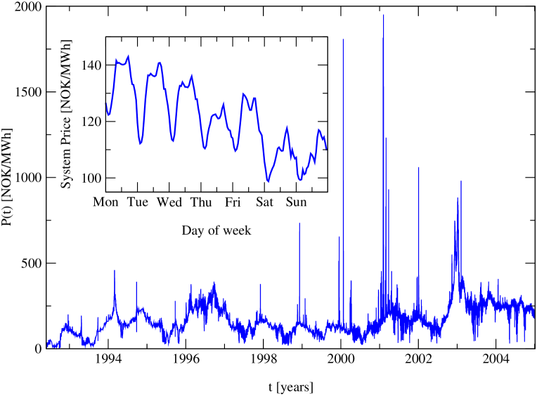
Figure 1: The Nord Pool system spot price from May, 1992 till the end of 2004. Several (seasonal, weekly, and daily) periodicities can be observed in this data set below the spiky randomness. The inset shows the price variations over a (randomly chosen) weekly period.

After having determined the system price, $P(t)$, for a given next-day hour, Nord Pool looks for potential bottlenecks (grid congestions) in the power transmission grid that might result from this system price. If no bottlenecks are found, the system price will represent the spot price for the whole Nord Pool area for that given hour. On the other hand, if potential grid congestions may result from the bidding, so-called area (spot) prices, that are different from the system price, will have to be created. The idea behind the introduction of area prices is to adjust electricity prices within a geographical area in order to favor local trading to such a degree that the limited capacity of the transmission grid is not exceeded. How the area prices are being determined within Nord Pool differs between, say, Sweden and Norway, and we will not discuss it further here (see e.g. Ref. [18] for details).

In this work, we will analyze the hourly Nord Pool system spot prices for the period from (Monday) May 4th, 1992 till the end of Friday December 31st, 2004; in total 110,987 data points (Fig. 1). In Fig. 2 we present the corresponding normalized hourly returns (to be defined in Eq. (6) below). The reader should notice that high levels of return are possible, and typical, for electricity markets. From Fig. 1 one should also observe that the price process shows several periodicities. Those are mainly attributed to consumption patterns and are daily, weekly and seasonal in character. They have been reported and studied previously by several research groups [8, 13, 19, 20, 21] Superimposed onto this deterministic periodic trend, is a random component showing strong variability with pronounced spikes and data clustering. The DEA technique allows us to deal with this randomness by somewhat ignoring the periodic signal.

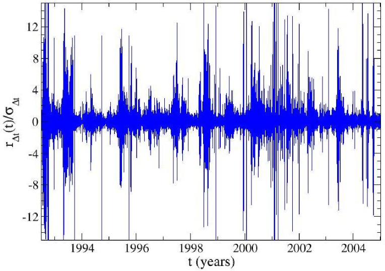
Figure 2: The normalized Nord Pool hourly ($\Delta t=1$ hour) (logarithmic) returns, $r_{\Delta t}(t)/\sigma_{\Delta t}$ (cf. Eq. (6)), of the data depicted in Fig. 1. The normalization is done according to the average hourly volatility $\sigma_{\Delta t}$. Notice that normalized return values higher than $10$ is rather frequent and typical for this (and many other) electricity markets.

3 The Diffusion Entropy Analysis

The DEA technique is a statistical method for measuring scaling exponents of time series by utilizing their thermodynamical properties [11, 12]. This is achieved by (i) converting the time series into some kind of probability density function (pdf), $p(x,t)$, where the variable $x$ is related to the fluctuating time series and $t$ denotes the time (or time interval), and (ii) therefrom calculating the related Shannon (information) entropy $S(t)$ (to be defined below), from which the scaling properties (if any) of the pdf can be deduced (cf. Eqs. (1) and (3) below).

Various pdf’s of the form $p(x,t)$, obtained from the underlying time series, can be used together with the DEA technique. For instance, $p(x,t)$ can be the probability of being at position $x$ at (diffusion) time $t$ given that one was at $x=0$ at time $t=0$, or $x$ may be a “marker” related to the number of events (like values of the time-series being above a given threshold etc.) occurring within a time interval of length $t$. Having said that, it should be mentioned that generally $x$ should be a zero-mean variable in order to avoid artifacts in the application of the DEA [11, 12]. We will in the preceding section describe in more details how one may construct a suitable pdf to be used in the DEA.

Under the assumption that the time series is stationary and scale invariant, one has that the pdf can be written as

$$p(x,t)=\frac{1}{t^{\delta}}\,F\left(\frac{x}{t^{\delta}}\right),$$ (1)

where $\delta$ denotes the so-called scaling exponent (that one wants to determine), and $F$ is some positive and integrable function depending on the specificities of the pdf. Then the Shannon entropy, that in general is defined as

$$S(t)=-\int_{-\infty}^{\infty}\mathrm{d}x\;p(x,t)\,\ln[p(x,t)],$$ (2)

will take on the form

$$S(t)=A+\delta\ln t,$$ (3)

where $A$ is given by an expression similar to Eq. (2), but with $F(y)$ substituted for $p(x,t)$. This last transition is easily demonstrated by substituting Eq. (1) into Eq. (2) and making a change of variable to $y=x/t^{\delta}$.

The important lesson that should be taken from Eq. (3) is that the scaling exponent, $\delta$, can be obtained as the slope of the entropy vs. $\ln t$ curve. This is a reliable method [9, 11, 12] for measuring the scaling exponent of the probability density (1).

4 Spikes and data clustering

One of the most pronounced features of the electricity spot price process of Fig. 1 is its spiky nature. Within one, or only a few hours, the spot price can increased manifold. One of the most extreme example of such a situation occurred on February 5, 2001, when the spot price reached an all-time-high of $1951.76$ NOK/MWh. Three hours earlier, the spot price had been at about $200$ NOK/MWh, a more “normal” level for that time of year.

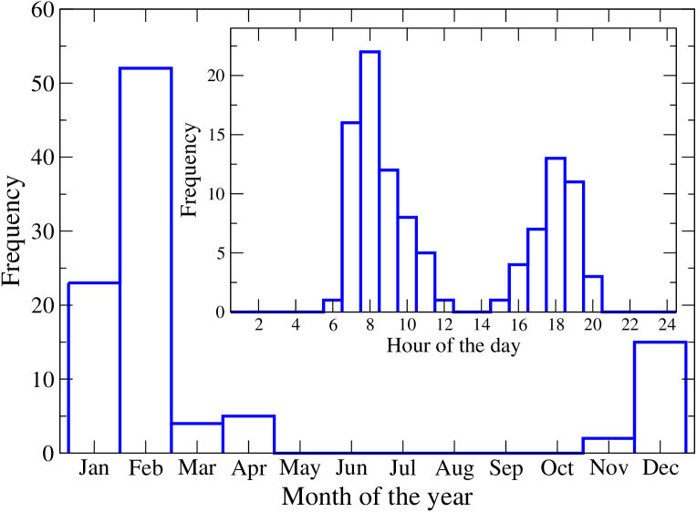
Figure 3: The frequency distributions of the $100$ largest hourly return events vs. month of year and hour of the day (inset) based on the data depicted in Fig. 2. This result clearly indicates that the dramatic price changes are not evenly distributed in time, but instead occur during periods of high consumption.

The dramatic price variations take place during periods of high consumption, which for the Nordic area means during the winter season as illustrated by Fig. 3. One way to explain the appearance of these dramatic price changes is by the so-called stacking or inventory models [22]: Extra demand for electric power is normally filled by the cheapest available energy source. During low consumption periods, the daily consumption profiles, say, will not influence the price level in any dramatic way, since there is plenty of base energy generation capacity available. However, when the consumption already is high, only a minor increase in the demand can have dramatic consequences for the electricity prices. The higher the demand, the more costly will it typically be to produce an extra unit of energy, and the more sensitivity will the price of electric power be to minor changes in the consumption. If one during such high-consumption periods experiences loss of less costly generating capacity, e.g. due to technical problems, extreme situations like the one reported above can be experienced. This sensitivity of the spot price to the level of consumption implies seasonal volatility clustering with typical low and high volatility periods during the summer and winter seasons, respectively [19].

The fact that the extreme price spikes are more likely to occur during the winter season than during the remaining parts the year, has the immediate consequence that time intervals between (consecutive) spikes are not expected to constitute a Poisson process. Hence, the time intervals are expected to scale anomalously according to Feller [23], and hence the scaling exponent will be different from $1/2$. This waiting time statistic (between spikes) has previously been studied in e.g. Ref. [9] for solar flares or earthquakes. It is worth mentioning that although the presence of seasonalities in spike statistics is quite evident looking at Fig. 3, this does not mean that the spike events follow a somewhat deterministic rule. As we will show later, time between spikes $\tau$ appears to be described by a power law probability distribution. The periodicities affect the statistics of very particular values of $\tau$ but not the whole probability density function.

It has in the past been demonstrated [12] that if the “spike” events are independent and the time interval between them distributed (at least asymptotically) according to a power law of the form ($\beta>0$)

$$\phi(\tau)\sim 1/\tau^{\beta},$$ (4)

then an analytic relationship between the $\beta$ and the scaling exponent $\delta$ do exist. For instance, if one constructs an auxiliary process by introducing steps, say, of magnitude $1$, whenever the originally set has absolute returns larger than a given threshold (called a marker below), the relationship reads [12]

$$\delta_{\rm spikes}=\cases{\beta-1,&if \ $1<\beta\leq 2$;\cr 1/(\beta-1),&if \ $2<\beta\leq 3$;\cr 1/2,&if \ $\beta>3$.}$$ (5)

Under this scope, the present section investigates the predictive power of the DEA analysis applied to the spike statistics of the Nordic electricity market. From the hourly system spot prices data, $P(t)$, one defines the logarithmic returns over the time horizon, $\Delta t$, as

$$r_{\Delta t}(t)\equiv\ln\left(\frac{P(t)}{P(t-\Delta t)}\right),$$ (6)

and in the following it will be assumed that $\Delta t=1$ hour. We intend to investigate the properties and time distribution of those returns being larger than a certain lower threshold $r_{0}$. To this end, we define a time-dependent marker position variable by

$$\xi(t)=\cases{1,&if \ $|r_{\Delta t}(t)|>r_{0}$,\cr 0,&otherwise.}$$ (7)

One now wants to estimate (count) the number of markers, $\tilde{y}_{t}(T)$, over a time interval $T$ ending at time $t$. With Eq. (7), this can readily be done by

$$\tilde{y}_{t}(T)=\sum\limits_{i=t-T}^{t}\xi(i),$$ (8)

and by subtracting the arithmetic average of this process one gets

$$y_{t}(T)=\tilde{y}_{t}(T)-\left<\tilde{y}_{t}(T)\right>_{t}.$$ (9)

If we vary the value of $t$ along the interval $[T,N\Delta t]$, where $N$ is the total number of data points of the analyzed sequence. From the knowledge of $y_{t}(T)$, one can now readily calculate the probability density function $p(y,T)$ for the moving counter.

At this point we apply the DEA technique [11, 12]. For each time-window of size $T$, one calculates the probability density function of $y_{t}$, that is: we get $p(y,T)$ for several $T$’s. The related (Shannon) entropy, $S(T)$, is then defined in accordance with Eq. (2). In Fig. 4 we present the behavior of the Nord Pool entropy (using the marker defined in Eq. (7)) for different values of threshold $r_{0}$. It is observed that the entropy, $S(T)$, scales in accordance with Eq. (3), and that the scaling exponent is found to be around $\delta_{\rm spikes}=0.91$ for all thresholds (solid line in Fig. 4). See Table 1 for further details on the fitting procedure.

It is interesting to notice that a similar value (within the error bars) for the scaling exponent has previously been reported for the activity of the US Dollar–Deutsche Mark futures market (using tick-by-tick data) [24] as well as for daily index data from the Dow Jones Industrial Average [25]. Hence, the Nordic power market has similar entropy growth to these two markets. Furthermore, all these data sets have comparable clustering.

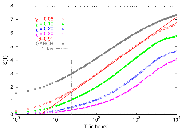
Figure 4: The results of the DEA of the Nord Pool spot price data using as marker $|r_{\Delta t}(t)|>r_{0}$ (with $\Delta t=1$ hour) for different thresholds $r_{0}$. The value of $\delta_{\rm spikes}$ is practically constant and, therefore, periodicities do not affect this kind of data analysis. For the GARCH curve, we take $r_{0}=0.2$ and we shift the results to see clearly. We have also added a vertical line to distinguish the intraday regime. The entropy there is highly affected by the consumption patterns of human activity.

Table 1: Regressions for the diffusion entropy results given in Fig. 4 assuming an entropy of the form $S(t)=A+\delta_{\rm spikes}\ln t$. Last column gives the time domain over which the regression is made.

• $r_{0}$	$\delta_{\rm spikes}$	data points	time range in hours
  0.05	$0.913\pm 0.002$	57	$40-2,000$
  0.10	$0.911\pm 0.008$	47	$100-2,000$
  0.20	$0.918\pm 0.008$	33	$200-2,000$
  0.30	$0.91\pm 0.01$	20	$500-2,000$

As was alluded to in the introduction to this section, the DEA technique aims at measuring the inhomogeneity of the distribution of the number of events (as defined by a marker) over a fixed period of time $T$, and to obtain the related scaling exponent $\delta$. An alternative (indirect) approach to obtaining the scaling exponent is to measure the tail exponent $\beta$ of the waiting time distribution $\phi(\tau)$, and apply relation (5) in order to obtaining the scaling exponent (under the stated assumptions).

Figure 5 depicts the pdf of waiting times between two consecutive spikes, $\phi(\tau)$, for different choices of the threshold $r_{0}$. It is mostly consistent with a decaying power-law of the form (5). There seems to be a slight dependence of the waiting time exponent $\beta$ on the choice of threshold, particularly for the largest waiting times $\tau$. One in Table 2 therefore presents the measured value of $\beta$ for the thresholds used. The corresponding scaling exponent obtained according to Eq. (5), is given in the last column of Table 2. One notices that the two methods — the direct via the diffusion entropy, and the indirect determination from the spike waiting time distribution — are consistent within the error-bars.

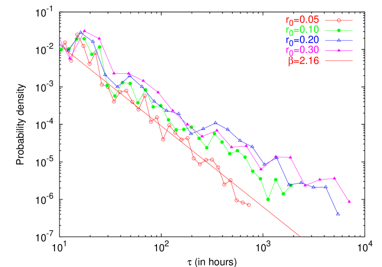
Figure 5: The waiting time pdf, $\phi(\tau)$, vs. the time interval between spikes, $\tau$, defined according to $|r_{\Delta t}(t)|>r_{0}$ (with $\Delta t=1$ hour) for different values of the threshold $r_{0}$ as indictaed in the legend. The data collapse for the different curves towards a decaying power law, $\phi(\tau)\sim 1/\tau^{\beta}$, is reasonably good. The individually measured waiting time exponents $\beta$ are given in Table 2. The solid line corresponds to a power-law fit with $\beta=2.16\pm 0.07$ for the threshold $r_{0}=0.05$.

Table 2: Regressions for the tail of the waiting time pdf $\phi(\tau)\sim 1/\tau^{\beta}$ between spikes larger than a certain threshold $r_{0}$. The fit provides the estimated exponent $\beta$ (see Eq. (4)) over the data plotted in Fig. 5. Last column corresponds to the scaling exponent $\delta$ predicted from the measured values of $\beta$ and assuming Eq. (5) to be right.

• $r_{0}$	$\beta$	data points	Predicted $\delta_{\rm spikes}$
  0.05	$2.16\pm 0.07$	39	$0.86\pm 0.05$
  0.10	$2.10\pm 0.30$	11	$0.85\pm 0.17$
  0.20	$1.84\pm 0.15$	11	$0.84\pm 0.15$
  0.30	$1.79\pm 0.12$	11	$0.79\pm 0.12$

5 Mean reversion and consumption patterns

There is in the literature wide consensus on the fact that electricity prices are stationary in the sense of suffering a reverting force driving price towards a normal level [1, 2, 5, 6, 8, 20, 21, 22, 26]. This level is most often time dependent due to marked consumption pattern in electricity prices caused by human social activity, and climatic factors like temperatures (see e.,g. Fig. 3). We will now for consistency address the mean reverting character of the Nordic spot electricity prices, but now using the DEA technique. Previously, using the AWC techniques, the so called Hurst exponent, $H$, characterizing this property, has been measured to be about $0.4$ [8], a similar value also found for the Californian electricity market [1].

For preparing for the use of the DEA for the measurement of the Hurst exponent, we define simply the “marker” being equal to the hourly returns, that is

$$\xi(t)=\ln(P(t)/P(t-\Delta t))=r_{\Delta t}(t).$$ (10)

The corresponding moving counting then, in analogy with Eqs. (8) and (9), reads

$$y_{t}(T)=\sum\limits_{i=t-T}^{t}r_{\Delta t}(t)=\ln P(t)-\ln P(t-T)=r_{T}(t),$$ (11)

where one in the last transition has used the definition of the return (6).

Figure 6 presents the (Shannon) entropy (2) of the moving counter $\xi(t)=r_{\Delta t}(t)$. It is observed that the stationary state is reached after about $5,000$ hours which corresponds to almost seven months. The signal will diffuse anomalously until it feels that the motion of $r_{\Delta t}(t)$ is constrained by the reverting force. After this threshold, the entropy $S(T)$ remains constant and the asymptotic scaling will be $\delta=0$ (cf. Eq. (3)) and the signal loses its memory.

According to Fig. 6 there also exists a transient state for shorter times than $T=5,000$ hours. In this regime, the DEA detects the presence of daily and weekly periodicities but it seems to be insensitive to seasonalities. The analysis, excluding the periodicities, also allows a fit like the one given by Eq. (3), that is

$$S_{\rm fit}=A+\delta_{\rm return}\ln T,$$ (12)

where in this case $\delta_{\rm return}$ equals the Hurst exponent $H$ use to the hourly returns being used as markers. From Fig. 6 it is observed that the DEA calculated entropy can be well fitted in time by the Hurst exponent

$$H_{\rm DEA}=\delta_{\rm return}=0.411\pm 0.002,$$ (13)

for the range between 100 and 6,000 hours. This result fully coincides with the Hurst exponent measured previously with the AWC method [8]. If the Hurst exponent $H=\delta_{\rm return}$ was equal to $1/2$ we would talk about a (ordinary) diffusion process with a standard deviation growing like $\sqrt{T}$. Therefore, finding a value smaller than $1/2$ for the Hurst exponent $H=\delta_{\rm return}$ means that the process is antipersistent or anticorrelated [23].

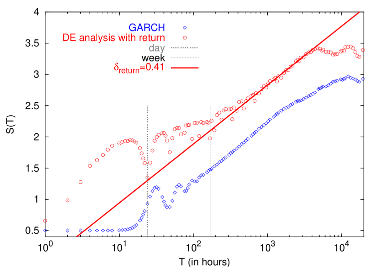
Figure 6: The result of DEA using $\xi(t)=r_{\Delta t}(t)$ as marker. The vertical lines signal the time of the main periodicities. We perform the analysis with the empirical data and a simulation of a GARCH model (14). The two time series have the same growth with time although for short time lags entropy differs due to the presence of periodicities in the original electricity spot prices.

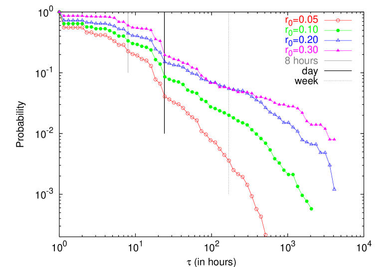
Figure 7: The complementary cumulative distribution of inter-spike waiting times, $\Phi(\tau)=1-\int_{\infty}^{\tau}d\tau^{\prime}\phi(\tau^{\prime})$. One observes that the decay of these distributions are different in several regions. This can be attributed to the presence of periodicities in the system spot prices. The slope changes are important in 8 hours and day (24 hours) time lags but are not unobservable in a week time lag.

Going further into the issue of periodicities, we now again explore the distribution of spikes distance $\tau$ for different thresholds. We display in Fig. 7 the complementary cumulative probability of this random variable. Compared to probability density plotted at Fig. 5 we note that the complementary cumulative distribution function of the spikes distance is greatly distorted by the presence of periodicities in the underlying data which breaks a possible power law collapse for several decades. This is mainly due to the gap in eight hours and daily periodicities while weekly effects does not affect very much the cumulative curve. These distortions are consistent with the periodicities detected by the DEA technique. It is again difficult to see the seasonal effects but clearly detect the rest of periodicities.

6 A GARCH type model

We have seen that the spike statistics for the electricity prices is very similar to that of the Dow Jones index and also to the peak statistics of the US Dollar–Deutsche Mark futures market [24, 25]. They both have the same data clustering. The analogy leads us to search for good candidates for price models for electricity in a similar way to as was done successfully in Refs. [24, 25]. Volatility clustering and mean reversion are among the essential characteristics of the volatility and of the market activity. Henceforth, our survey focuses on existing volatility models.

A possible new attempt is to propose a GARCH model [16] for the spot price. We suggest the following model for the system spot price $P(t)$:

$$P(t)=k+\chi P(t-\Delta t)\eta^{2}+\nu P(t-\Delta t),$$ (14)

where $\eta$ denotes uncorrelated gaussian random noise of zero mean and unit variance. Using this GARCH theoretical model, with parameters $\chi=4\times 10^{-4}$, $\nu=0.9994$ and $k=0.00184$ NOK/MWh, one can simulate long time series that results in an $S(T)$ dependence that resembles that of the real Nord Pool market (Fig. 4). To obtain the results of Fig. 4 the total length of the simulated and real data were the same, and that the markers $|r_{\Delta t}(t)|>r_{0}$ were used. This model can generate $\delta_{\rm spikes}\simeq 0.9$ thus giving similar entropy profile to the electricity spot price data.

In addition, we also performed the DEA for the logarithmic return time series, generated by Eq. (14) using the parameters given above, and markers defined in Eq. (10). Figure. 6 shows that this GARCH model produces results for the diffusion entropy that are consistent with real data. Specifically, the transient period resulting from the model time series has the same exponent and the stationary state is approached simultaneously with the real electricity return time series. Moreover, if Eq. (14) is rewritten in terms of the price difference $\Delta P(t)=P(t)-P(t-\Delta t)$

$$\Delta P(t)=-(1-\nu)\left[P(t-\Delta t)-\frac{k}{1-\nu}\right]+\chi P(t-\Delta t)\eta^{2},$$ (15)

we can observe that the reverting force has a characteristic time scale $\hat{\tau}=1/(1-\nu)$. It is directly related to $\nu$ and brings us the value $\hat{\tau}=1,667$ hours (more than 2 months) which is of the same order of the time required for real data to arrive at the stationary state. The ratio $k/(1-\nu)$ represents the normal level that prices are driven toward. In case, one would like to include the consumption patterns in the model one should replace $k$ by a periodic signal. Finally, the $\chi$ value sets the magnitude of the fluctuations. Having a big $\chi$ means having wild fluctuations of price.

7 Conclusions

By applying the DEA technique we have shown that the entropy of the Nordic electricity spot prices grows with the size of the time window in a similar way to the volatility and the market activity as different as the Dow-Jones and the US Dollar–Deutsche mark futures. The DEA scaling parameter has the similar value $\delta_{\rm spikes}\sim 0.9$ and they have a comparable clustering.

We have also shown that the distribution of waiting times of the electricity price scales as $\phi(\tau)\sim 1/\tau^{\beta}$ given by Eq. (4) and that the corresponding power-law exponent $\beta$ is related to the DEA parameter $\delta_{\rm spikes}=0.91\pm 0.01$ as anticipated by the DEA – see Eq. (5) and Fig. 5. The relationship derived in Ref. [12] is obtained under the hypothesis that spikes are uncorrelated. This hypothesis might hold true or not but in any case we have found that the relationship between $\beta$ and $\delta_{\rm spikes}$ is still applicable in the Nord Pool case.

We have also obtained a Hurst exponent ($\delta_{\rm return}=0.412\pm 0.002$) with the DEA technique which is coincident with the one derived by previous studies and using different techniques. The resulting quantity implies an antipersistent behaviour of electricity prices. Moreover, we have been able to detect, for hourly prices, a characteristic time scale around $5,000$ hours in which the system reaches the stationary state.

Due to the several similarities in statistical properties with financial markets, a GARCH model was proposed and investigated for the spot electricity prices. In particular, it was shown that the diffusion entropy of such a theoretical GARCH model followed surprisingly closely the entropy that was obtained for the Nord Pool system spot prices.

We finally mention that although the DEA seems to detect daily and/or weekly periodicities in the analyzed data, a more thorough investigation is required to settle this issue. Efforts are currently undertaken to address this topic.

References

References

- [1] Weron R and Przybylowicz B, 2000 Physica A 283 462
- [2] Weron R, in Measuring long-range dependence in electricity prices, 2002 Empirical Science of Financial Fluctuations ed H Takayasu (Tokyo: Springer-Verlag) pp 110–19
- [3] Hurst H E, Black R P and Simaika Y M, 1965 Long Term Storage: An Experimental Study (London: Constable)
- [4] Peng C-K, Buldyrev S V, Havlin S, Simons N, Stanley H E and Goldberger A L, 1994 Phys. Rev. E 49 1685
- [5] Schwartz E S, 1997 J. Fin. 52 923
- [6] Clewlow L and Strickland C, 2000 Energy Derivatives — Pricing and Risk Management, (London: Lacima Publications)
- [7] Simonsen I, Hansen A and Nes J M, 1998 Phys. Rev. E 58 2779
- [8] Simonsen I, 2003 Physica A 322 597
- [9] Grigolini P, Leddon D and Scaffeta N, 2002 Phys. Rev. E 65 046203
- [10] Metzler R and Klafter J, 2000 Phys. Rep. 339 1
- [11] Scafetta N, Hamilton P and Grigolini P, 2001 Fractals 9 193
- [12] Grigolini P, Palatella L and Raffaelli G, 2001, Fractals 9 439
- [13] Escribano Á, Peña J I and Villaplana P, Modelling electricity prices: International Evidence, Working paper 02-27, Economics Series 08, June 2002, Departamento de Economía, Universidad Carlos III de Madrid
- [14] Engle R F, 1982 Econometrica 61 987
- [15] Bollerslev T, Chou R Y and Kroner K F, 1992 J. Econometrics 52 5
- [16] Engle R F and Patton A J, 2001 Quant. Fin. 1 237
- [17] Duffie D, Gray S and Hoang P, 1998 Volatility in Energy Prices, Managing Price Risk (RiskPublications, 2nd ed.)
- [18] See NordPools’s web-page: http://www.nordpool.no. This is a good staring point for additional information on the Nordic Power Exchange.
- [19] Simonsen I, 2005 Physica A 355 10
- [20] Pilipovic D and Wengler J, 1998 Energy and Power Risk Management 2 22
- [21] Lucía J and Schwartz E, 2002 Review of Derivatives Research 5 5
- [22] Weron R, Simonsen I and Wilman P, 2004 Modeling highly volatile and seasonal markets: evidence from the Nord Pool electricity market, in The Application of Econophysics ed H Takayasu (Tokyo: Springer-Verlag) pp 182–91
- [23] Feller W, 1949 Trans. Am. Math. Soc. 67 98
- [24] Palatella L, Perelló J, Montero M and Masoliver J, 2004 Eur. Phys. J. B 38 671
- [25] Palatella L, Perelló J, Montero M and Masoliver J, 2005 Physica A 355 131
- [26] Weron R, Kozlowska B and Nowicka-Zagrajek J, 2001 Physica A 299 344