Abstract

This paper introduces a new concept of one-dimensional hologram which represents one line image, and a new kind of display structure using it. This one-dimensional hologram is similar to a superpositioned diffraction lattice. And the interference patterns can be efficiently computed with a simple optical computing structure. This is a Proposal for a new kind of display method.

OCIS codes: 090.2870, 090.1760.

1 Introduction

This paper intends to introduce a new display method using the holography theory by Dennis Gabor in 1948. The holography had been expected to be a popular display method for a 3-dimensional image, but the burden of tremendous amount of data processing prohibited the practical application. Thus, I would like to introduce a one-dimensional holographic display concept which can reduce the burden of data processing, can adopt simple optical computing method, and has some more practical merits in manufacturing. A one-dimensional hologram can display only a two-dimensional image, but it does not require the lenses like HMD(Head Mount Display). Instead, this one-dimensional holographic display device has a possibility of showing a real-time two-dimensional information without a lens, within today’s technology.

This paper contains theoretical considerations about the one-dimensional Holography, and the equations that I derived showing the existence of the one-dimensional hologram as well as discussions about practical structures of the display device, the light modulators, and the optical computing device.

This work had started by considering the information dimension of a hologram. A traditional two-dimensional hologram can display a three dimensional image, So I speculated that this 2 to 3 relationship between data dimension and image dimension could be transformed into 1 to 2 relationship. So, I first tried to find a one-dimensional hologram for a two-dimensional image by geometrical method, but failed. Instead, I found that a diffraction lattice like one-dimensional hologram is formed by some special condition of line image. And, I had conceived a vector and matrix based mathematical technique which can easily express the idea. Unexpectedly, this technique was also useful to handle the problem of diffraction efficiency and noise cancelling problem for computed artificial two-dimensional hologram.

2 The Hologram

A phasor expression for a wave from one point source is Eq. (1).

Let $A(\vec{r})$ represent the relative phase and the amplitude of a wave function, then

$$A(\vec{r})=\alpha(\vec{r})\exp{(i[f(\vec{r})+\delta])}$$ (1)

($\alpha(\vec{r})=\sqrt{\mbox{the detection probability of wave quanta}}$ , $f(\vec{r})=2\pi r/\lambda$ ) The $\alpha$ is indeed a complex function, but when $r\gg\lambda$, it is a simple function proportional to $1/r$, and it is actually a constant when computing a one-dimensional hologram mainly discussed in this paper. The traditional wave function $\Psi$ is obtained by considering the time term. $\Psi(\vec{r},t)=A(\vec{r})\exp(2\pi i\omega t)$ The above phasor expression does not represent a real wave, but the interference pattern of a certain point depends on only relative phase differences between light rays, so the time term disappears when computing the interference pattern. The coherent rays have constant relative phases. The polarization of lights are ignored. A phasor expression for waves from many point sources is Eq. (2) by the principle of superposition.

Let $S(\vec{r})$ be superpositioned $A(\vec{r})$ of Eq.(1), then

$$S(\vec{r})=\sum\alpha(\vec{r})\exp{(i[f(\vec{r})+\delta])}$$ (2)

An actual hologram is a record of the interference pattern on a photographic plate. The interference pattern depends on the illumination.

Let $I(\vec{r})$ be the illumination over the space then,

$$I(\vec{r})=\left|S(\vec{r})\right|^{2}=\left|\sum\alpha(\vec{r})\exp{(i[f(\vec{r})+\delta])}\right|^{2}$$ (3)

This can be rewritten as

$$I(\vec{r})=\sum\alpha(\vec{r})\exp{(i[f(\vec{r})+\delta])}\times\sum\alpha(\vec{r})\exp{(-i[f(\vec{r})+\delta])}$$ (4)

And, when expanded to a matrix, it is

$$I(\vec{r})=\left(\begin{array}[]{ccccc}\alpha_{1}^{2}&\alpha_{1}\alpha_{2}e^{i(f_{1}-f_{2})}&\alpha_{1}\alpha_{3}e^{i(f_{1}-f_{3})}&\alpha_{1}\alpha_{4}e^{i(f_{1}-f_{4})}&\cdots\\ \alpha_{2}\alpha_{1}e^{i(f_{2}-f_{1})}&\alpha_{2}^{2}&\alpha_{2}\alpha_{3}e^{i(f_{2}-f_{3})}&\alpha_{2}\alpha_{4}e^{i(f_{2}-f_{4})}&\cdots\\ \alpha_{3}\alpha_{1}e^{i(f_{3}-f_{1})}&\alpha_{3}\alpha_{2}e^{i(f_{3}-f_{2})}&\alpha_{3}^{2}&\alpha_{3}\alpha_{4}e^{i(f_{3}-f_{4})}&\cdots\\ \alpha_{4}\alpha_{1}e^{i(f_{4}-f_{1})}&\alpha_{4}\alpha_{2}e^{i(f_{4}-f_{2})}&\alpha_{4}\alpha_{3}e^{i(f_{4}-f_{3})}&\alpha_{4}^{2}&\cdots\\ \cdots&\cdots&\cdots&\cdots&\cdots\end{array}\right)$$ (5)

This matrix needs normalization for actual application, but the image reproduction with a hologram may now be certified. If you select $\alpha_{1}\exp(if_{1}(\vec{r}))$ as reference light and illuminate it as reproducing light(select $\alpha_{1}=1$ for intensity) on a hologram which represents the above matrix, then $J(\vec{r})$ represents the modulated lights,

$$J(\vec{r})$$ (11)

$$= I(\vec{r})\exp{(if_{1}(\vec{r}))}$$

$$= \left(\begin{array}[]{ccccc}e^{if_{1}}&\alpha_{2}e^{i(2f_{1}-f_{2})}&\alpha_{3}e^{i(2f_{1}-f_{3})}&\alpha_{4}e^{i(2f_{1}-f_{4})}&\cdots\\ \alpha_{2}e^{if_{2}}&\alpha_{2}^{2}e^{if_{1}}&\alpha_{3}\alpha_{3}e^{i(f_{1}-(f_{3}-f_{2}))}&\alpha_{2}\alpha_{4}e^{i(f_{1}-(f_{4}-f_{2}))}&\cdots\\ \alpha_{3}e^{if_{3}}&\alpha_{3}\alpha_{2}e^{i(f_{1}+(f_{3}-f_{2}))}&\alpha_{3}^{2}e^{if_{1}}&\alpha_{3}\alpha_{4}e^{i(f_{1}-(f_{4}-f_{3}))}&\cdots\\ \alpha_{4}e^{if_{4}}&\alpha_{4}\alpha_{2}e^{i(f_{1}+(f_{4}-f_{2}))}&\alpha_{4}\alpha_{3}e^{i(f_{1}+(f_{4}-f_{3}))}&\alpha_{4}^{2}e^{if_{1}}&\cdots\\ \cdots&\cdots&\cdots&\cdots&\cdots\end{array}\right)$$

Take this matrix’s diagonals to the first term, remaining first column to the second term, remaining first row to the third term, and others are added to their symmetry conjugated and defined by cosine function, then the result is

$$J(\vec{r}) = \exp{(if_{1}(\vec{r}))}(1+\sum\alpha^{2})$$ (13)

$$+\sum\alpha\exp{(if(\vec{r}))}$$

$$+\sum\alpha\exp{(i[2f_{1}(\vec{r})-f(\vec{r})])}$$

$$+2\exp{(if_{1}(\vec{r}))}\sum\alpha_{m}\alpha_{n}\cos(f_{m}(\vec{r})-f_{n}(\vec{r}))$$

The first term is 0th order term, the second term represents image, the third term represents conjugate image, and the fourth term is noise term. The above method does not depend on any particular coordinate system, so it can explain volume hologram, as well.

3 The One-dimensional Hologram

When considering the dimensions of storing and displaying hologram, the volume hologram can display three-dimensional image, and can be multiplexed with wavelengths and spatial coordinates of light sources. The two-dimensional hologram can display three-dimensional image, and can not be multiplexed. When considering one-dimensional hologram, one-dimensional hologram can display one-dimensional image(one-line image), and can not be multiplexed.

In Cartesian coordinate system, when $r\gg\lambda$, Eq. (1) can be rewritten as

$$A(\vec{r}) = A(X,Y,Z)$$ (14)

$$= \frac{\alpha}{r}\exp{(2\pi i[{\frac{\sqrt{(Ox-X)^{2}+(Oy-Y)^{2}+(Oz-Z)^{2}}}{\lambda}}+\delta])}$$

($\sqrt{(Ox-X)^{2}+(Oy-Y)^{2}+(Oz-Z)^{2}}=r$, $(Ox,Oy,Oz)$ is the coordinate of dot light source) This expression represents a volume hologram’s case. The two-dimensional hologram formation on a $XY$ plain can be obtained by substitution $Z=0$. The thickness of zero can not exist in real world, so an actual two-dimensional hologram by photographic method is a thin volume hologram and in fact, it is significantly advantageous to reduce image noise.

If $Y$ is substituted with zero again, it could be called as a one-dimensional hologram. But, it is a hologram on a physical line. It is hard to find physical meaning. Instead, if a hologram on a plain is expressed with single axes information, then it also can be called as the one-dimensional hologram.

The phase of Eq. (8) is relative to the source of light. It is possible to transform the expression to be relative to the origin $(X,Y,Z)=(0,0,0)$ of coordinate system. When the light is parallel, the $r$ of Eq. (1) is infinite, $r_{0}$ is the distance between the origin and source.

$$A(\vec{r}) = A(X,Y,Z)$$

$$= \frac{\alpha}{r}\exp{(2\pi i[\frac{r(x,y,z)-r_{0}}{\lambda}+\delta])}$$

$$= \frac{\alpha}{r}e^{\textstyle 2\pi i[\frac{\sqrt{(Ox-X)^{2}+(Oy-Y)^{2}+(Oz-Z)^{2}}-\sqrt{Ox^{2}+Oy^{2}+Oz^{2}}}{\lambda}+\delta]}$$

$$\approx \frac{\alpha}{r}\exp{(2\pi i[\frac{-\frac{OxX+OyY+OzZ}{\sqrt{Ox^{2}+Oy^{2}+Oz^{2}}}}{\lambda}+\delta])}$$

$$= \frac{\alpha}{r}\exp{(-2\pi i[\frac{\frac{\textstyle\vec{r}\cdot\hat{x}X+\vec{r}\cdot\hat{y}Y+\vec{r}\cdot\hat{z}Z}{\textstyle r}}{\lambda}+\delta])}$$

$$= \frac{\alpha}{r}\exp{(-2\pi i[\frac{\textstyle\hat{r}\cdot\hat{x}X+\hat{r}\cdot\hat{y}Y+\hat{r}\cdot\hat{z}Z}{\lambda}+\delta])}$$

When $r=\infty$, $\alpha/r$ can be changed to constant $\alpha$, therefore

$$A(X,Y,Z)=\alpha\exp{(-2\pi i[\frac{\hat{r}\cdot\hat{x}X+\hat{r}\cdot\hat{y}Y+\hat{r}\cdot\hat{z}Z}{\lambda}+\delta])}$$

Now, one dimension can be reduced by limiting $XY$ plain with $Z=0$. Therefore the result is,

$$A(X,Y)=\alpha\exp{(-2\pi i[\frac{\hat{r}\cdot\hat{x}X+\hat{r}\cdot\hat{y}Y}{\lambda}+\delta])}$$ (15)

($\alpha\exp{(-2\pi i[\frac{\textstyle\hat{r}\cdot\vec{P}}{\lambda}+\delta])}$ is more adept for final result, but Eq. (9) shall be used for convenience) According to the method of Eq. (2), the expression for many points is

$$S(X,Y)=\sum\alpha\exp{(-2\pi i[\frac{\textstyle\hat{r}\cdot\hat{x}X+\hat{r}\cdot\hat{y}Y}{\lambda}+\delta])}$$

At this time, when $\hat{r}\cdot\hat{y}=c$(onstant) (all the points are on same latitude in polar coordinate), the above can be rewritten as

$$S(X,Y)=\exp{(-2\pi i\frac{\hat{r}\cdot\hat{y}}{\lambda}Y)}\sum\alpha\exp{(-2\pi i[\frac{\hat{r}\cdot\hat{x}}{\lambda}X+\delta])}$$ (16)

The real hologram information is obtained by applying the method of Eq. (4) for Eq. (10). Let $\alpha_{1}=1$, then the result is,

$$I(X,Y)$$ (21)

$$= |S(X,Y)|^{2}$$

$$= \exp{(-2\pi i\frac{\hat{r}\cdot\hat{y}}{\lambda}Y)}\sum\alpha\exp{(-2\pi i[\frac{\hat{r}\cdot\hat{x}}{\lambda}X+\delta])}$$

$$\times\exp{(2\pi i\frac{\hat{r}\cdot\hat{y}}{\lambda}Y)}\sum\alpha\exp{(2\pi i[\frac{\textstyle\hat{r}\cdot\hat{x}}{\lambda}X+\delta])}$$

$$= \sum\alpha\exp{(-2\pi i[\frac{\hat{r}\cdot\hat{x}}{\lambda}X+\delta])}\times\sum\alpha\exp{(2\pi i[\frac{\textstyle\hat{r}\cdot\hat{x}}{\lambda}X+\delta])}$$

$$= I(X)$$

$$= \left(\begin{array}[]{cccc}1&\alpha_{2}e^{2\pi i\frac{\textstyle(\hat{r_{1}}-\hat{r_{2}})\cdot\hat{x}}{\textstyle\lambda}X}&\alpha_{3}e^{2\pi i\frac{\textstyle(\hat{r_{1}}-\hat{r_{3}})\cdot\hat{x}}{\textstyle\lambda}X}&\cdot\\ \alpha_{2}e^{2\pi i\frac{\textstyle(\hat{r_{2}}-\hat{r_{1}})\cdot\hat{x}}{\textstyle\lambda}X}&\alpha_{2}^{2}&\alpha_{2}\alpha_{3}e^{2\pi i\frac{\textstyle(\hat{r_{2}}-\hat{r_{3}})\cdot\hat{x}}{\textstyle\lambda}X}&\cdot\\ \alpha_{3}e^{2\pi i\frac{\textstyle(\hat{r_{3}}-\hat{r_{1}})\cdot\hat{x}}{\textstyle\lambda}X}&\alpha_{3}\alpha_{2}e^{2\pi i\frac{\textstyle\!(\hat{r_{3}}\!\!-\hat{r_{2}}\!)\!\cdot\hat{x}}{\textstyle\lambda}X}&\alpha_{3}^{2}&\cdot\\ \cdots&\cdots&\cdots&\cdot\end{array}\right)$$

The term of $Y$ was cancelled. So, this is expressed with one-dimensional data which depend on $x$ axes only. Therefore, Eq. (11) represents a one-dimensional hologram in this paper. According to the method of Eq. (5),(6), the modulation of reproducing light is

$$J(X,Y)$$

$$= \exp{(-2\pi i\frac{\hat{r}_{1}\cdot\hat{x}X+\hat{r}_{1}\cdot\hat{y}Y}{\lambda})}$$

$$\left(\begin{array}[]{cccc}1&\alpha_{2}e^{2\pi i\frac{\textstyle(\hat{r_{1}}-\hat{r_{2}})\cdot\hat{x}}{\textstyle\lambda}X}&\alpha_{3}e^{2\pi i\frac{\textstyle(\hat{r_{1}}-\hat{r_{3}})\cdot\hat{x}}{\textstyle\lambda}X}&\cdot\\ \alpha_{2}e^{2\pi i\frac{\textstyle(\hat{r_{2}}-\hat{r_{1}})\cdot\hat{x}}{\textstyle\lambda}X}&\alpha_{2}^{2}&\alpha_{2}\alpha_{3}e^{2\pi i\frac{\textstyle(\hat{r_{2}}-\hat{r_{3}})\cdot\hat{x}}{\textstyle\lambda}X}&\cdot\\ \alpha_{3}e^{2\pi i\frac{\textstyle(\hat{r_{3}}-\hat{r_{1}})\cdot\hat{x}}{\textstyle\lambda}X}&\alpha_{3}\alpha_{2}e^{2\pi i\frac{\textstyle\!(\hat{r_{3}}\!\!-\hat{r_{2}}\!)\!\cdot\hat{x}}{\textstyle\lambda}X}&\alpha_{3}^{2}&\cdot\\ \cdots&\cdots&\cdots&\cdot\end{array}\right)$$

And, sorting as Eq. (7), results are

$$J(X,Y)$$

$$= \exp{(-2\pi i\frac{\hat{r}_{1}\cdot\hat{x}X+\hat{r}_{1}\cdot\hat{y}Y}{\lambda})}(1+\sum\alpha^{2})\mbox{......................................\{1\}}$$

$$+\sum\alpha\exp{(-2\pi i\frac{\hat{r}\cdot\hat{x}X+\hat{r}_{1}\cdot\hat{y}Y}{\lambda})}\mbox{..............................................\{2\}}$$

$$+\sum\alpha\exp{(-2\pi i\frac{(2\hat{r}_{1}-\hat{r})\cdot\hat{x}X+\hat{r}_{1}\cdot\hat{y}Y}{\lambda})}\mbox{..................................\{3\}}$$

$$+2\exp{(-2\pi i\frac{\hat{r}_{1}\cdot\hat{x}X+\hat{r}_{1}\cdot\hat{y}Y}{\lambda})}\sum\alpha_{mn}\cos{(2\pi\frac{(\hat{r}_{m}-\hat{r}_{n})\cdot\hat{x}X}{\lambda})}\mbox{...\{4\}}$$

($\delta$ is omitted) Also, {1} is term of 0th order, {2} is a term representing the image, {3} is a term representing the conjugated image, which confirms that it works as a hologram. Some of the lights expressed by terms of {3} and {4}, may not be reproduced because the final unit vectors of light ray always have to satisfy the size of 1. This means, for example, among the lights of term {3}, the lights those $((2\hat{r}_{1}-\hat{r})\cdot\hat{x})^{2}+(\hat{r}_{1}\cdot\hat{y})^{2}$ are smaller than 1, can be generated.

It is the same situation of a diffraction grating that is expressed with grating equation¹ $\alpha(\sin{\theta_{m}}-\sin{\theta_{i}})=m\lambda$. In grating equation, the degree of $\pm m$ is limited as the absolute value of a sinusoidal function is limited to 1.

Term {2} can have physical meaning with different wavelengths or latitude angles of incidence, so it is impossible to multiplex the one-dimensional hologram by wavelengths or latitude angles of incidence.

4 The one-dimensional holographic display device

The one-dimensional hologram may be used to make a display device as described in figure 1.

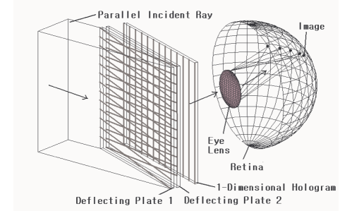
Fig. 1: An example of one-dimensional hologram display device.

To reproduce a image, a one-dimensional hologram should be expressed with a spatial light modulator and a proper reproducing light should be illuminated, then one line of image shall be displayed. And, the whole plain image is displayed by updating the one-dimensional hologram and the angle of incidence( $\hat{r}_{1}\cdot\hat{y}$ of Eq. (12) term {2}) of the parallel reproducing light synchronously and in sequence. The natural color is obtained by repeating display with the three primary colors.

The incident angle of reproducing light should be adjustable, so a deflection device is needed. There may be many kind of deflection device, but the one-dimensional hologram itself also can be used as a deflector. In fact, the one-dimensional hologram deflector is identical to a cosine diffraction lattice.

The deflecting plate 1, 2 and the one-dimensional hologram are cross structured light modulators. One of the deflecting plate 1 or 2 operates at a time and the other maintains the transparent state. The incident angle of parallel ray in figure 1 is fixed as in figure 2, then one of the deflectors 1 and 2 deflects the parallel ray by deflection range 1 or 2 in figure 2.

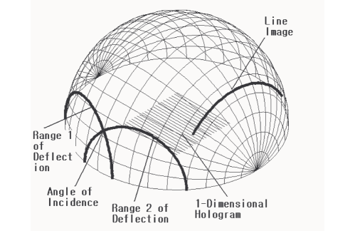
Fig. 2: Deflection ranges of deflecting plates, and displaying image.

This structure makes it possible to eliminate the 0th order light by total internal reflection. It is considerable to replace one of the one-dimensional hologram deflectors with a multiplexed volume hologram.

Theoretically, it is possible to display a two-dimensional image with above scheme, but there are some more considerable problems to actually develop and operate this display device. They are developing optical modulation device, noise cancelling of image, and the fast computation of the interference pattern. And, the comparison with conventional two-dimensional hologram method or with controllable diffraction lattice method is needed to verify the usefulness of the one-dimensional hologram display method.

4.A The light modulating device

A hologram display device requires very high resolution spatial light modulator than conventional display device. Recently, it had been announced that liquid crystal display device has reached the resolution of $10\mu m$. However, this resolution is still not enough to display a hologram.

The hologram method display device has no relation between the image resolution and the resolution of optical modulation device. The resolution of modulator is related to the field of view, precisely, it is related to the angle between a light from a picture element of an image and the reference light of hologram. When $\alpha_{1}=1$, Eq. (11) can be rewritten as,

$$I(X)$$ (29)

$$= \left(\begin{array}[]{cccc}1&\alpha_{2}e^{2\pi i\frac{\textstyle(\hat{r_{1}}-\hat{r_{2}})\cdot\hat{x}}{\textstyle\lambda}X}&\alpha_{3}e^{2\pi i\frac{\textstyle(\hat{r_{1}}-\hat{r_{3}})\cdot\hat{x}}{\textstyle\lambda}X}&\cdot\\ \alpha_{2}e^{2\pi i\frac{\textstyle(\hat{r_{2}}-\hat{r_{1}})\cdot\hat{x}}{\textstyle\lambda}X}&\alpha_{2}^{2}&\alpha_{2}\alpha_{3}e^{2\pi i\frac{\textstyle(\hat{r_{2}}-\hat{r_{3}})\cdot\hat{x}}{\textstyle\lambda}X}&\cdot\\ \alpha_{3}e^{2\pi i\frac{\textstyle(\hat{r_{3}}-\hat{r_{1}})\cdot\hat{x}}{\textstyle\lambda}X}&\alpha_{3}\alpha_{2}e^{2\pi i\frac{\textstyle\!(\hat{r_{3}}\!\!-\hat{r_{2}}\!)\!\cdot\hat{x}}{\textstyle\lambda}X}&\alpha_{3}^{2}&\cdot\\ \cdots&\cdots&\cdots&\cdot\end{array}\right)$$

$$= 2\sum\sum\alpha_{m}\alpha_{n}\cos{(2\pi\frac{\textstyle(\hat{r}_{m}-\hat{r}_{n})\cdot\hat{x}X}{\lambda})}$$ (30)

This shows that a hologram is the sum of spatial periodic structures which is expressed with $\lambda/(\hat{r}_{m}-\hat{r}_{n})\cdot\hat{x}$. The possible maximum value of $(\hat{r}_{m}-\hat{r}_{n})\cdot\hat{x}$ is 2 and at least two pixel is needed to express one spatial period, so, the resolution of light modulator should be $\lambda/4$ to display a image without the limitation of visual field. To express natural color, if about $400nm$ of blue ray wavelength is substituted for $\lambda$, then a modulator of approximately $100nm$ resolution is required. When using previously mentioned liquid crystal display device of $10\mu m$ resolution as spatial light modulator, from $\frac{\textstyle 400nm}{\textstyle 2(\hat{r}_{m}-\hat{r}_{n})\cdot\hat{x}}=10\mu m$, the maximum field of view is $(\hat{r}_{m}-\hat{r}_{n})\cdot\hat{x}=\frac{\textstyle 400nm}{\textstyle 2\times 10\mu m}=0.02$, this is capable of displaying about $2cm$ wide virtual screen at $1m$ distance, which has no practical use. Fortunately, there have been continuous researches for other types of optical modulation devices. As one of them, according to recently opened Japan NTT Docomo’s patent document², they have mentioned that higher than $1\mu m$ resolution may be obtained by using a photo-refractive crystal. This is capable of displaying about $20cm$ wide screen at $1m$ distance, but still it is not fully enough.

The $1\mu m$ resolution mentioned above is the possible resolution for the two-dimensional hologram. The resolution of modulator can be improved by using one-dimensional hologram. To display a two-dimensional hologram, one pixel electrodes should be placed for each pixel, each electrode should have a controlling circuit, each circuit should have at least two interface wires, all these elements should be placed on a transparent plate with a matrix form. Figure 3 is a light modulation device structure for hologram display suggested by NTT Docomo.

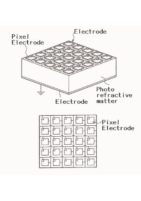
Fig. 3: NTT Docomo’s light modulator.

To display a one-dimensional hologram, all the structures mentioned above may not be placed on the displaying transparent plate, except the pixel electrodes. Displaying the figure 4 clearly doesn’t need the matrix of figure 3.

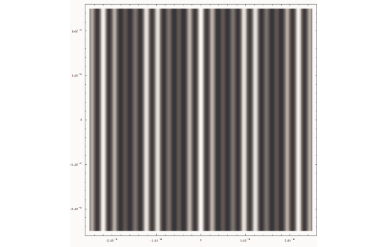
Fig. 4: An example of one-dimensional Hologram.

Only the pixel electrodes are needed to be placed for display and all other elements may be placed at the edge of each electrode. This will improve the display resolution almost to the limit of wiring technology. It seems that the recent $60nm$ wiring technique is enough for the goal of $100nm$ resolution.

4.B The noise eliminating in hologram calculation

A practical display device needs to consider about the problem of image quality. The image quality is determined by resolution of image, luminosity and noise. The resolution problem shall not be discussed, because the holography is intrinsically high resolution display, regardless of the modulator’s resolution. And, the luminosity problems may be solved by multiple modulating of phase modulation method. Then the noise remains.

The 4th term of Eq. (7) and term {4} of Eq. (12) are the noise terms. These noises are caused from the assumption that light modulation happens instantly at a surface. When reproducing light is illuminated to hologram of Eq. (11), the energy distribution $E$ of all modulated lights by hologram without normalization is

$$E=\left(\begin{array}[]{ccccc}1&\alpha_{2}^{2}&\alpha_{3}^{2}&\alpha_{4}^{2}&\cdots\\ \alpha_{2}^{2}&(\alpha_{2}\alpha_{2})^{2}&(\alpha_{2}\alpha_{3})^{2}&(\alpha_{2}\alpha_{4})^{2}&\cdots\\ \alpha_{3}^{2}&(\alpha_{3}\alpha_{2})^{2}&(\alpha_{3}\alpha_{3})^{2}&(\alpha_{3}\alpha_{4})^{2}&\cdots\\ \alpha_{4}^{2}&(\alpha_{4}\alpha_{2})^{2}&(\alpha_{4}\alpha_{3})^{2}&(\alpha_{4}\alpha_{4})^{2}&\cdots\\ \cdots&\cdots&\cdots&\cdots&\cdots\end{array}\right)$$ (31)

When the number of image elements is $n$ and assuming that all image elements have identical luminosity for convenience, the Eq. (14) can be rewritten as $E=1+n\alpha^{2}+n\alpha^{2}+n^{2}\alpha^{4}$. The first term is the 0th order term except diagonals, the second term is the total luminosity of image, third term is the total luminosity of conjugate image and fourth term is sum of 0th order diagonals and noise term. when $\alpha\rightarrow 0$ with same $n$ the total luminosity of image is sufficiently less than reference light, the energy of noise term becomes negligible than the energy of image. This shows that the noise term is especially important for the computer generated hologram on a plain, and negligible when a volume hologram is used. But, noise can be eliminated by simply throwing the noise term and using row 1 and column 1 of Eq. (5), except diagonals. That is, instead of the expression of Eq. (3)

$$I(\vec{r})=\left|\sum\alpha(\vec{r})\exp{(i[f(\vec{r})+\delta])}\right|^{2}$$

, by adding row 1 and column 1 those elements are complex conjugates with one another. So, it is expressed with cosine function.

$$I(\vec{r})=2\alpha_{1}(\vec{r})\sum\alpha(\vec{r})\cos(f_{1}(\vec{r})-f(\vec{r})+\delta_{1}-\delta)$$ (32)

Applying Eq. (15) to (11) to get expression of one-dimensional hologram,

$$I(X)=2\sum\alpha\cos(2\pi\frac{\textstyle(\hat{r}_{1}-\hat{r})\cdot\hat{x}X}{\lambda}+\delta_{1}-\delta)$$ (33)

The negative value becomes possible, so, it needs different way for normalization. This one-dimensional hologram can be called as multiplexed cosine diffracting lattice.

4.C Fast hologram computing

One of the most big problem in hologram display device is its tremendous data processing burden. When displaying 3-D image with a hologram, there is no other way except improving the algorithm, but when displaying 2-D image, it is possible to compute only partial area of modulator, and can reuse its data on whole area to improve the speed of computing. When using one-dimensional holography, this situation becomes better. For two-dimensional hologram, all the hologram pixels ($\mbox{column H(ologram) pixels}\times\mbox{row H pixels}$) must be computed by all the image pixels($\mbox{column I(mage) pixels}\times\mbox{row I pixels}$). But, For one-dimensional, just one column of the hologram pixels(column H pixels) are computed by one column of the image pixels(column I pixels), and repeats this for number of the row line of image(row I pixels). This increases computing speed by

$$\frac{\mbox{column H pixels}\times\mbox{row H pixels}\times\mbox{column I pixels}\times\mbox{row I pixels}}{\mbox{column H pixels}\times\mbox{column I pixels}\times\mbox{row I pixels}}$$

equals

row H pixels

The aperture size of human eyes¹ are between $2mm$ to $8mm$. So, for clean visuality, let the size of partial hologram to be $2mm$, and let the hologram resolution to be $100nm$, then the one-dimensional hologram may be computed 20,000 times faster than the 2-D displaying two-dimensional hologram. But, current digital calculator may not be able to handle the required computing burden for real time color motion picture display.

Fortunately, there is other solution for one-dimensional hologram calculation. It is possible to make adjustable one-dimensional interference pattern then read it with photo-sensor array.

A coherent light started from a source is modulated and diffused by light modulation device with input signal, this light is modulated into multiple parallel rays by lens, and gain hologram output data by reading interference patterns from those parallel rays with photo-sensor array. This is shown on figure 5.

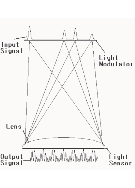
Fig. 5: The optical computing structure.

In this case, the calculation speed depends on the speed of sufficient light gathering at the photo-sensor, a laser has sufficient power with care of only generated heat. The reference light was not indicated on figure 5. It is out of range from radical axis, so, it can not be illuminated through the lens, it should be illuminated diagonally from $z$ axis direction. In this case, the noise removing method of Eq. (16) can’t be used, so, small values of $\alpha$ should be used. In order to do so, A multi-layered one-dimensional hologram may be used. The light modulation efficiency should be lowered at each hologram, and the modulation is repeated with multiple layer.

When looking at expression from Eq. (11),

$$I(X)=\sum\alpha\exp{(-2\pi i[\frac{\hat{r}\cdot\hat{x}}{\lambda}X+\delta])}\times\sum\alpha\exp{(2\pi i[\frac{\hat{r}\cdot\hat{x}}{\lambda}X+\delta])}$$

it shows that only $\hat{r}\cdot\hat{x}$ values are used for one-dimensional hologram calculation. Therefore, the structure of figure 5 can be applied to all latitude lines regardless of $\hat{r}\cdot\hat{y}$. Also because, reducing $\hat{r}\cdot\hat{x}$ value and properly increasing $X$ value results in same, so, input pixels can be changed to more paraxial, and at the same time, it makes the size of the photosensor array larger. The method in figure 5 can be formed in a thin shape with tens thousand pixel lineal CCD in one-dimensional holography, but when applied to two-dimensional hologram, it would encounter the problems of embodying in a thick shape, illuminating the reference light very out of ranged from radical axis, and making hundreds million pixel CCD.

4.D The comparison with diffraction lattice

As mentioned above, a one-dimensional hologram can be regarded as a multiplexed diffraction lattice, too. So, the comparison of one-dimensional and diffraction lattice is considerable.

When examining the calculation speed of diffraction lattice to display an image, for a diffraction lattice, each column of the lattice line pixel ( column L pixels) should be computed by each pixels of the image, and this should be repeated for the number of the row lines of image ( row I pixels), then repeated again for the number of the column lines of image ( column I pixels). This amount of calculation equals to that of the one-dimensional hologram.

Considering the computing speed, diffraction lattice is not bad, but there are other problems in diffraction lattice method. The light modulator for displaying the diffraction lattice should be changed for each image pixels. When one line image of one-dimensional hologram consists of 2000 pixels, the modulator for diffraction lattice should be reconfigured 2000 times more than one-dimensional hologram. This means that the light modulator and all the elements of figure 5 should have 2000 times faster speed than those of one-dimensional hologram.

To compare the data transfer rate, let us assume that light modulator consists of $1mm\times 1mm$ parts by $100nm$ resolution, the displaying image consists of $2000\times 2000$ pixels, and let us choose the frame rate of 48 frames per a second(24 is traditional frame rate, but a hologram or a lattice can express only one color at a time, thus some extra frames are needed. It seems that 72 monochrome frames are not required for 24 color frames, when 6 frames are used for three times of shape refreshing, and two times of color refreshing, 48 frames are enough. 48 is chosen because it is about 50 that is easy to handle.), then the time limit for a frame of two-dimensional hologram is about $1s/50=20ms$, for a line frame of one-dimensional hologram is about $1s/50/2000=10\mu s$, and for a dot frame of the diffraction lattice is $1s/50/2000/2000=5ns$.(A $2000\times 2000$ pixel image is quite high resolution for plain pictures, but it is only not so bad resolution for eyeglasses type display devices of wide visual angle.) And, with $1mm/100nm=10000$, the transfer rates are calculated as $10000\times 10000/20ms=5$ giga times per a second for two-dimensional hologram, $10000/10\mu s=1$ giga times for one-dimensional hologram, and $10000/5ns=2$ tera times for diffraction lattice. These results show that the one-dimensional holography is most efficient.

Some other ways of using diffraction lattice exist they avoid calculation and transmission of data. A material which self arranges its fringe by voltage has been known, and the method of using acoustic wave as the diffraction lattice also has been known. But, the arrangement speeds of these methods seem difficult to meet $5ns$ of time limit, because the state of molecules in that kind of material should be determined by their neighbour molecules, and the informations are exchanged with the speed of acoustic wave. The acoustic wave method may be considerable for one-dimensional holography, if it is capable of expressing $100nm$ resolution.

5 Conclusion

The one-dimensional holography is a new display method which has balanced characteristics between conventional two-dimensional holography and diffraction lattice method. This is a theoretical method yet, and thus it seems that there are no precedent and few references. But, this is not a unique theory, this is an application of common theory for a special problem, thus, this could be theoretically verified easily.

Many researcher’s dedications are required for practical use of one-dimensional holography. Especially, the research for a fast responsive light modulating material seems essential. As modulating method, phase modulating or polarization modulating material may be adequate. Also, more precise design of optical calculator is required. Other computing methods like analog computing device or faster DSP could be researched. And, many others may also be needed.

References

• [1] Eugene.Hecht ,Optics 4/ed(Doo-Yang Sa(Kor.) / (Addison Wesley Longman, San Francisco, Calif., 2002)
• [2] Horikoshi Tsutomu, Fukumoto Masaaki, Sugimura Toshiaki and Tsuboi Masafumi ” SOLID IMAGE DISPLAY APPARATUS AND SYSTEM(JP,2005-099738,A)” (Japan Patent Office, Tokyo, Japan, 2005)
• [3] Young-Cheol Kim, β€œAppling 1 Dimensional Hologram to Display Device” in Journal of The Institute of Electronics Engineers of Korea Proceedings on Semiconductors and Devices (The Institute of Electronics Engineers of Korea, Seoul, Korea 2005), pp. 561–570.