String Theory and Einstein’s Dream

Ashoke Sen

Harish-Chandra Research Institute

Chhatnag Road, Jhusi, Allahabad 211019, INDIA

E-mail: ashoke.sen@cern.ch, sen@mri.ernet.in

1 Introduction

Unification of the theory of gravitation, as given by Einstein’s general theory of relativity, and the theory of electromagnetism, as formulated by Maxwell, had been Einstein’s dream during the later part of his life. String theory, which is the subject of this article, is an attempt to realize this dream. However in many ways string theory attempts to go beyond Einstein’s dream. String theory attempts to bring all known forces of nature, – not just gravity and electromagnetism, – under one umbrella. It also tries to do so in a manner that is consistent with the principles of quantum mechanics, – the theory that is necessary for describing the laws of nature at very small distance. Thus string theory is an attempt to provide an all encompassing description of nature that works at large distances where gravity becomes important as well as small distances where quantum mechanics is important.

In this article I shall try to give a very general introduction to string theory. However in order to do so, I must begin by reviewing our current understanding of the basic constituents of matter. This is the subject to which we shall now turn.

2 The World of Elementary Particles

According to our current understanding, everything that we see around us is made of a few elementary building blocks. Figure 1 gives us a bird’s eye view of our current knowledge of the structure of matter. At the crudest level the building blocks of matter are the individual molecules of various compounds. However there are a very large number of compounds, each with its own characteristic molecule. A simpler picture emerged when it was realized that each molecule is made of some smaller building blocks known as atoms. There are about 100 different types of atoms and different molecules differ in their properties because they contain different number of atoms of different types in different arrangements. During the early years of the twentieth century it was realized that atoms are also not the smallest constituents of matter, – each atom is made of a central nucleus and a set of electrons revolving around it. Different atoms have different number of electrons, but all the electrons found in all atoms have identical properties. In contrast the nuclei of different types of atoms have very different properties. This picture simplified once it was realized that each nucleus can be regarded as being made of even smaller constituents, – the proton and the neutron. Different nuclei have different properties because they contain different numbers of protons and neutrons. Finally, even the protons and neutrons are now known to be made of even smaller constituents called quarks – the proton being made of two up ($u$) quarks and one down ($d$) quarks, and the neutron of one $u$ and two $d$ quarks. According to our current knowledge, the electrons and the quarks cannot be divided any further. We call them elementary particles.

Figure 1: Our current understanding of the building blocks of matter.

This gives us a very simple picture of the structure of matter, namely everything is made of three different types of ‘elementary particles’ – the electron, the $u$ quark and the $d$ quark. However as we shall see, this is far from a complete picture. As is already evident from Fig. 1, the up and down quarks each come in three varieties. Here we have denoted them by $u_{1}$, $u_{2}$, $u_{3}$ and $d_{1}$, $d_{2}$, $d_{3}$, but often they are refered to as red, blue and green type of quarks. We shall refer to this as the colour quantum number although this has nothing to do with the colour that we see in everyday life. The quarks inside the proton and neutron continuously change their colour due to a process known as strong interaction that will be discussed soon. There are various other reasons why this picture is not complete. I shall review some of them here.

In order to understand the structure of matter, we need to understand not only the basic constituents of matter, but also the nature of the forces that operate between them. Without this knowledge we shall not have any understanding of what keeps the quarks bound inside a proton and neutron, or at a larger scale, of what keeps the atoms bound inside a molecule. According to our current knowledge there are four basic types of forces operating between elementary particles, – 1) gravitational, 2) electromagnetic, 3) strong and 4) weak. Of these the gravitational and the electromagnetic forces are familiar to us from everyday experience. For example the gravitational force is responsible for earth’s gravity and the motion of the planets around the sun. The electromagnetic force is the cause of lightening in the sky, the force of a magnet, working of various electrical appliances etc. It is also responsible for binding the electrons and the nuclei inside the atom and the atoms inside a molecule. The strong force operates between quarks and is responsible for binding them inside a proton and a neutron and also for binding the proton and the neutron inside a nucleus. The weak force, being weak, is not responsible for binding any particles; however it is responsible for certain radioactive decays known as $\beta$-decay.

It turns out that in studying the physics of elementary particles, we can ignore the effect of gravitational force. To see this one can compare the electrostatic force between two protons with the gravitational force between two protons at rest. The result is

$${\hbox{Grav. Force}\over\hbox{Elec. Force}}={G_{N}m_{p}^{2}/r^{2}\over e_{p}^{2}/r^{2}}\sim 10^{-36}$$

where $G_{N}$ is the Newton’s constant ($6.67\times 10^{-8}$ cm³/gm sec²) that controls the strength of the gravitational force between two bodies, $m_{p}$ is the proton mass ($1.67\times 10^{-24}$ gm) and $e_{p}$ is the proton charge ($4.8\times 10^{-10}$ e.s.u.). Clearly this ratio is extremely small. Similarly all other forces can also be shown to be much larger than the gravitational force.

Figure 2: Classical picture of the deflection of a pair of electrons via electromagnetic force.

So far we have discussed the elementary particles and the forces operating between them as separate entities, but with the help of quantum theory one can give a unified description of elementary particles, and the forces among the elementary particles. Consider for example the electromagnetic force between two electrons when they pass each other. Due to this force, each particle gets deflected from its original trajectory. This has been depicted in Fig. 2. In quantum theory, one provides a different explanation of the same phenomenon. Here the deflection takes place because the two electrons exchange a new particle, called photon, while passing near each other (see Fig. 3). The photon is capable of carrying some amount of energy and momentum from the first electron to the second electron, thereby causing this deflection. We call the photon the mediator of electromagnetic force. Even though it mediates electromagnetic force, the photon itself is electrically neutral.

Figure 3: Quantum picture of the deflection of a pair of electrons via electromagnetic force.

Thus in the language of quantum theory we can describe a force by specifying the particle(s) which mediate the force. It turns out that the strong force is mediated by eight different particles known as gluons. These particles are all electrically neutral. The quarks inside a proton (and neutron) continuously exchange gluons, and in this process keep changing their colour quantum number. On the other hand the weak force is mediated by three particles, denoted by $W^{+}$, $W^{-}$ and $Z$. $W^{+}$ and $W^{-}$ carry +1 and -1 unit of electric charge respectively while $Z$ is neutral. (The unit of electric charge is taken to be the charge carried by a single proton. Thus $W^{+}$ has charge equal to that of a proton, while $W^{-}$ has charge that is equal in magnitude but opposite in sign to that of a proton.)

Clearly, we must add the gluons, $W^{+}$, $W^{-}$ and $Z$, as well as the photon, to our list of elementary particles. We shall refer to these as the mediator particles. Theoretical analysis shows that for every elementary particle there must also be another elementary particle, known as the antiparticle, that carries exactly the same amount of charge but with opposite sign. Thus for every quark and the electron we have the corresponding anti-quark and the anti-electron (known as the positron). Fortunately the gluons, the photon and the $Z$ particles are their own anti-particles, whereas $W^{-}$ is the anti-particle of $W^{+}$ and vice-versa. Thus we do not need to expand our list by including anti-particles of the mediator particles. However this still does not exhaust the list of all elementary particles. Besides the $u$ and $d$ quarks, electrons and mediators and their anti-particles, there are also other elementary particles which are produced by cosmic rays, radioactive decays, collision of high energy particles, etc. They must also be added to the list.

Our current list contains about 100 types of elementary particles. Thus the situation would not seem any better than the days when atoms were thought to be the basic constituents of matter. The properties of matter known at that time could be explained in terms of the properties of about 100 types of atoms. There is however a difference, – unlike the case of atoms, there is a simple mathematical theory that explains the properties of all the elementary particles. In fact this theory has been so successful that it has come to be known as the ‘standard model’ of elementary particles. This model, in principle, can be used to calculate the result of any experiment that we wish to perform involving the elementary particles. So far the standard model has been extremely successful in explaining almost all experimental results.

3 The Standard Model: Its Successes and Limitations

In this section I shall explain some of the basic properties of the standard model. The basic inputs in this theory are

• quantum mechanics,

• special theory of relativity, and

• laws of electromagnetism and their generalization to strong and weak forces.

There is a mathematical framework, known as gauge theory, that includes all these three features. I shall not describe the details of this framework here. It turns out that there are many different consistent gauge theories, one of which describes the theory of elementary particles. This particular theory is known as the standard model.

Once the theory is written down, it predicts the outcome of every possible experiment involving elementary particles. (Of course some experimental inputs go in to decide on what is the right theory.) For example the standard model tells us precisely what kind of elementary particles we have in our world. According to this model, the elementary particles in our world fall into four categories:

• Quarks   $u_{1},u_{2},u_{3}$,  $d_{1},d_{2},d_{3}$,  $c_{1},c_{2},c_{3}$,  $s_{1},s_{2},s_{3}$,  $t_{1},t_{2},t_{3}$,  $b_{1},b_{2},b_{3}$

  In this list we recognize the familiar up and down quarks, each coming in three colours. It turns out that nature contains four more types of quarks, – charm ($c$), strange ($s$), top ($t$) and bottom ($b$), each coming in three colours. These four types of quarks are not usually found inside matter but can be produced in highly energetic collision among normal matter. Of the six quarks, the up, charm and top quarks carry 2/3 unit of electric charge, whereas the down, strange and bottom quarks carry $-1/3$ unit of electric charge. For each quark we also have its anti-quark; we have not listed them separately here.

• Leptons   $e^{-},\nu_{e}$,  $\mu^{-},\nu_{\mu}$,  $\tau^{-},\nu_{\tau}$

  In this list we recognize the electron ($e^{-}$); the $-$ sign on top is to remind ourselves that the electron carries $-1$ unit of charge, ı.e. charge equal in magnitude but opposite in sign to that carried by the proton. $\nu_{e}$, – known as the electron neutrino, – is a weakly interacting chargeless particle. These are so weakly interacting that a neutrino passing through the earth does so experiencing almost no force. The pair of particles$(\mu^{-},\nu_{\mu})$ have properties similar to that of the pair $(e^{-},\nu_{e})$ although the muon ($\mu^{-}$) is a lot heavier that the electron. Similarly the pair $(\tau^{-},\nu_{\tau})$ have properties similar to that of $(e^{-},\nu_{e})$, with the tau particle $(\tau^{-}$) being even heavier than a muon. For each lepton we also have an anti-lepton which we have not listed here. For example, the anti-particle of the electron is called the positron and denoted by the symbol $e^{+}$.

• Gauge Bosons  gluons: $g_{1},\ldots g_{8}$,  Photon: $\gamma$,  $W^{+}$, $W^{-}$, $Z$

  These are the by now familiar mediator particles which have been discussed before. As already mentioned the list is complete without having to add the anti-particles separately.

• Higgs Particle  $\phi$

  This is the most mysterious particle in the standard model. Unlike every other particle in the list which has been experimentally observed, the Higgs particle has never been seen in any experiment despite several attempts. Nevertheless its existence is predicted by the standard model, and new experiments are being designed to look for this particle.

Figure 4: An allowed process in the standard model.

The standard model not only gives us a list of elementary particles but also the list of processes that can occur involving these particles. For example in order to explain the electromagnetic force between electrons using the process described in Fig. 3, it is necessary to know that an electron can emit a photon. This follows from the mathematical framework that lies behind the standard model. The same mathematical framework also tells us that if in this diagram we replace the electron by an electron neutrino then this is not an allowed process in the standard model; hence a neutrino cannot exchange a photon with another particle. Fig. 4 shows another example of a process that can occur in the standard model. This describes the decay of a top quark ($t_{1}$) into an electron neutrino ($\nu_{e}$), a positron ($e^{+}$) and a bottom quark ($b_{1}$). In fact the standard model not only tells us which processes can occur, but it also gives us precise mathematical formula for calculating the probablility of occurance of any such process. These predictions are then compared with experimental data to test the model.

Given the success of the standard model, one might like to conclude that we now have a complete understanding of the elementary constituents of matter. This however is not true. There are several reasons why standard model cannot be the complete theory of elementary particles. I shall review a few of these here.

First and foremost, the standard model does not explain the origin of one of the important forces that we observe in nature, namely the gravitational force. In particular the list of particles predicted by the standard model does not contain any particle that mediates gravitational force. The effect of this omission of course is not seen in any of the experiments involving elementary particles since, as observed earlier in this article, the gravitational force between two elementary particles is extremely small compared to the other forces. Nevertheless a complete theory must account for every possible tiny effect that exists in nature. Thus a theory that does not provide an explanation of the gravitational force cannot be a complete theory of nature.

In order to appreciate the gravity of this problem, let us first take stock of what is known about gravity. Our current theoretical understanding of the gravitational force is based on the ‘general theory of relativity’, – a theory written down by Einstein almost a hundred years ago. This theory has been enormously successful in explaining all effects related to gravity. Unfortunately this theory is based on the principles of classical mechanics and not of quantum mechanics. Since other forces in nature follow the rules of quantum mechanics, any theory that attempts to explain gravity as well as the other forces of nature must treat gravity according to the rules of quantum mechanics. Hence the general theory of relativity, despite being so successful, cannot be the final story about gravity. In fact the reason that this theory has been so successful so far is that for gravity the difference between the predictions of a classical and the quantum theory is extremely tiny and cannot be observed in any of the current experiments. (We say that quantum effects involving gravity are extremely small.)

Thus the problem at this stage seems to be to first find a quantum theory of gravity and then combine this with the standard model to arrive at a complete theory of all elementary particles and forces operating between them. At the first sight the problem does not seem unsurmountable. After all, we normally obtain a quantum theory by first writing down a classical theory and then applying a definite set of rules to turn it into a quantum theory. Why can’t the same thing be done with the general theory of relativity? If one proceeds to do this one does get some encouraging results at first. In particular one finds that like other forces, gravity is also mediated by a new kind of elementary particle. This particle has been given the name graviton. Like the diagram in Fig. 3 one will have a diagram where two electrons exchange a graviton, representing the (tiny amount of) deflection of one of the electrons due to gravitational force of the other electron.

Figure 5: An infinite contribution to the gravitational scattering of two electrons.

So far everthing seems to be proceeding as desired. However one soon runs into a problem with this approach. To understand the origin of this difficulty consider the process shown in Fig. 5 involving multiple graviton exchanges. As in the case of the standard model, there are precise mathematical rules for computing the probability amplitude of this process in the quantum general theory of relativity. When one applies those rules to calculate this probability amplitude, one finds that the result is infinity!

This is clearly a nonsensical answer! In actual practice we know that this probability must be extremely tiny since no experiment has yet seen the effect of gravitational force between elementary particles. Thus there must be something wrong with this theory.

In order to appreciate how string theory eventually resolves this problem, it will be useful to investigate in a little more detail the origin of this problem. You would notice that in a diagram like the one shown in Fig. 5 there are ‘interaction vertices’ where three (or more) lines meet. For example in Fig. 5 there are four such interaction vertices. These are the points where something happens. We can regard these points as the basic events which make up the complete process. Each such event takes place at a given point in space at a given time, and in order to calculate the total probability amplitude of the process we must integrate over the location of each event in space as well as in time. It turns out that the integrand, calculated using the rules of quantum theory, diverges (becomes infinite) when more than two or more such elementary events take place at the same point in space at the same time. This in turn causes the integral to diverge occasionally.

In any case the final outcome of this complicated analysis is that the standard procedure that has been successful in formulating a quantum theory of strong, weak and electromagnetic forces do not work for gravity, and for this reason it is not easy to incorporate gravity into the standard model.

Besides the problem of incorporating gravity, the standard model suffers from other conceptual and technical problems. While it is true that the standard model, once formulated, can predict the results of most experiments involving elementary particles, the formulation of the theory itself requires a lot of input from experiments. For example there are many consistent gauge theories, often labelled by several continuous parameters, and standard model corresponds to one of these theories with a specific choice of the values of these parameters. There is no explanation within the theory as to why this particular gauge theory with this particular choice of parameters should describe our universe. Furthermore the choice of parameters which describes the standard model are not generic, but requires very fine tuning. This is evident from the fact that the theory has some extremely small dimensionless numbers like the ratio of gravitational and electromagnetic force between two elementary particles. For a generic choice of parameters this ratio would be of order one. Finally recent experiments show that not all predictions of the standard model are completely correct. In particular, according to the standard model the neutrinos are zero mass particles, but recent experiments show that neutrinos actually have a tiny but finite mass. This requires a small modification of the gauge theory that describes the standard model.

These are some of the reasons why we believe that the standard model is not the final story. In the rest of this article we shall try to see how string theory attempts to address some of these issues.

4 String Theory

The basic idea in string theory is quite simple. It says that the elementary constituents of matter are not point like objects (particles) but one dimensional objects. These one dimensional objects, also known as the fundamental (or elementary) strings, have very specific properties which determine the various modes in which the string can vibrate. However to the present day experimentalists these strings appear as particles since their size is small compared to the distance scale that can be probed by the most powerful microscopes available today. In particular, different vibrational states of a fundamental string appear to us as different elementary ‘particles’ just as the different modes of vibration of a single musical string can produce different harmonics of a note. Thus in string theory instead of having different types of elementary particles we have one single type of elementary string as the basic constituent of matter. Fig. 6 shows some of the vibrational states of strings. As is evident from this figure, strings can come in two varieties, – closed strings which have no boundary and open strings which have two end points forming its two boundaries.

Figure 6: Vibrating closed and open strings.

Since quantum mechanics and special theory of relativity are two of the basic inputs in the standard model, and since string theory must include the standard model if it is to describe our universe, it is natural to require that string theory also respects the principles of quantum mechanics and special theory of relativity. However one finds that for various technical reasons it is not easy to respect these principles. In fact the only way we can respect these principles is by formulating string theory not in the usual three dimensional space but in a hypothetical nine dimensional space. Furthermore in this nine dimensional space one can formulate altogether five different types of string theory, – known as the Type I, Type IIA, Type IIB, E${}_{8}\times$E₈ heterotic and SO(32) heterotic string theories. These five string theories differ from each other in the type of vibrations which the string performs. As a result they have different vibrational states, which is reflected in the spectrum of elementary ‘particles’ that each of these theories produce.

Having nine space dimensions instead of three seems to be a serious problem. We shall return to this issue shortly and show that this in fact is not a very serious problem. However, let us leave aside this problem for a moment and discuss some of the good things which string theory provides. First of all one finds that one of the vibrational states of string theory have properties identical to that of a graviton, – the mediator of gravitational force. Furthermore one finds that string theory calculations do not suffer from any infinities of the type we encounter while trying to directly quantize general theory of relativity. Thus string theory provides us with a finite quantum theory of gravity!

Figure 7: A process describing a pair of strings scattering from each other.

It is instructive to try to understand why the probability amplitudes calculated in string theory are finite. For this we need to look at the figure 7 describing the process of scattering of two strings. Like in the case of point particle theories, there are definite mathematical rules for calculating the probability amplitude of this process. The point to note is that in this diagram there are no points where specific events (like splitiing of a single string into a pair of strings) take place; the diagram is completely smooth everywhere. As a result the divergences in the point particle theories, – which arise when two or more such events take place at the same point at the same time, – are absent in string theory. This is the intuitive reason why string amplitudes are finite.

At this point we must mention that the graviton is only one of the many vibrational states of an elementary string. In fact the laws of quantum mechanics tells us that a single elementary string has infinite number of vibrational states. Since each such vibrational state behaves as a particular type of elementary particle, string theory seems to contain infinite types of elementary particles. This would be in contradiction with what we observe in nature were it not for the fact that most of these elementary particles in string theory turn out to be very heavy, and not observable in present experiments. Thus there is no immediate conflict between what string theory predicts and what we observe in actual experiments. On the other hand these additional heavy elementary particles are absolutely essential for getting finite answers in string theory.

Figure 8: A two dimensional space with a compact coordinate.

Let us now return to the issue about the dimension of space-time. Consistency of string theory demands that we can formulate the theory only in 9 space dimensions. How can string theory be relevant for describing nature, which seems to have only 3 space dimension? The answer to this question is provided by an old idea known as compactification. This idea was pioneered by Kaluza and Klein during the first half of the twentieth century and Einstein himself had been attracted by this idea. We shall illustrate the basic idea by a simple example in which we begin with a world with two space dimensions instead of nine space dimensions. We take the two space coordinates to describe the surface of a cylinder of radius R instead of an infinite plane as shown in Fig. 8. All objects (including light) in this world can move only along the surface of the cylinder. Thus if we move along the vertical direction in the figure, then after travelling a certain distance ($2\pi R$ where $R$ is the radius of the cylinder) we shall traverse the whole circumference of the circle and come back to the original point where we started. We call this a compact drection. In contrast an object can travel along the horizontal direction without ever returning to its original position and we call this the non-compact direction.

Figure 9: A two dimensional space with a small compact coordinate.

Clearly if $R$ is very large (larger than the range of the most powerful telescope) then the two dimensional space will appear to be infinite in both directions and we would not know that one of the directions is compact. If $R$ is within the visible range, then the two dimensional creatures will start seeing infinite number of images of each object separated by an interval of $2\pi R$ since light from any object can reach an observer in many (infinite number of) ways, – directly, travelling once around the circumference, travelling twice around the circumference etc. This may seem strange from our point of view but will not at all seem strange from the point of view of the two dimensional people living in this world since they would always see their world this way. But now consider the case when $R$ is very small, as shown in Fig. 9. Clearly this world looks one dimensional as $R\to$0. In fact as long as $R$ is smaller than the resolution of the most powerful microscope, the two dimensional people will never know that they have a hidden dimension in their world. To them the world will appear to be one dimensional.

This illustrates the way a universe with a certain number of space dimensions can ‘appear to be’ a universe with less number of dimensions. This idea can be generalized to make the nine dimensional world of string theory look like three dimensional world in which we live. All we need to do is to take six of the nine space directions to be small, describing a compact space $K$. When the size of K is sufficiently small, the space will appear to be 3 dimensional. The main difference with the two dimensional example that we discussed is that while there is only one one dimensional space (namely the circle) that can be used for making one direction compact, there are more possibilities in higher dimensions. An important class of six dimensional spaces which are useful for compactification of string theory are the so called Calabi-Yau spaces. There are many different six dimensional Calabi-Yau spaces, and the theory that describes the three dimensional world after compactification depends on the choice of the compact space $K$, as well as which of the five string theories we start from in nine dimensions.

Often the three dimensional theory found this way comes very close to describing the world we see around us. In particular when we examine the vibrational states of the string in such a space, not only do we find the graviton, but we often find ‘gauge bosons’, – the kind of particles which mediate strong, weak and electromagnetic forces. Some other vibrational states have properties similar to those of various quarks, leptons, Higgs particle etc. Thus string theory has the potential of describing a unified theory of elementary particles and all the forces operating between them.

We would like to emphasize here that in string theory we use quantum mechanics and special theory of relativity as basic inputs; but the general theory of relativity and gauge theories come out of string theory. Thus string theory in a sense provides an explanation of why the forces operating in our universe are described by general theory of relativity and gauge theories.

Of course all is not well at this stage. First of all, we have the problem that even though we know of many string compactifications which come very close to describing the world that we see, there is no known compactification that describes exactly the world that we see around us. Trying to look for a string compactification that describes exactly the theory that governs our universe is an active area of research in which many theorists are participating. Second, one might wonder what is the basic principle that one uses to decide which of the five string theories is the right theory for describing our universe. If we are looking for a theory that describes everything in our universe, wouldn’t it be nicer to have a single mathematically consistent theory rather than five consistent theories? Finally, even if there is some principle that tells us which of the five string theories we should use, there are still many different choices of the compact space that brings us down to three dimension; and one might wonder what principle decides on the choice of the compact space. In fact it is possible to have string compactification where the number of non-compact direction is different from three; all it requires to have $d$ non-compact directions is to choose an appropriate compact space of dimension $(9-d)$. Thus the question arises as to why our world is three dimensional? We shall try to address some of these issues in the next section.

5 Duality, M-theory and the Early Universe

So far we have discussed the role played by the vibrational states of a single fundamental string. However these are not the only possible objects in string theory. String theory contains many other types of objects which can be made of more than one (some time infinite number of) fundamental strings. We shall call these objects composite objects.

In conventional approach to the study of elementary constituents of matter, we make a clear distinction between elementary and composite objects. For example in the standard model the quarks are elementary particles while the proton and the neutron are composite particles made of quarks. The standard model tells us various properties of quarks and other elementary particles in the theory; the properties of protons, neutrons and other composite objects can be derived from the properties of these constituent particles. Thus elementary particles enjoy a previlaged position in the description of the theory.

The initial formulation of string theory was based on the same principle, with the role of elementary particles being taken over by the elementary strings. The vibrational states of the elementary string were the analogs of the elementary particles; all other objects made of more than one elementary strings were composite objects whose properties could in principle be derived from the properties of the elementary string. However this picture, that gives a special role to the elementary particles, got modified dramatically after the discovery of duality symmetries in string theory. This is the story to which we now turn.

During the mid 90’s it was realised that some time a pair of theories which ‘look’ different may actually describe the same physical theory. In other words, the same physical theory may have different descriptions as different compactifications of different string theories. This symmetry, relating the two apparently different theories, is known as the duality symmetry. This name is actually a misnomer, since often one finds more than two descriptions of the same physical theory. One of the surprising features of duality symmetries is that a particle which looks elementary in one description may appear as composite in a dual description. Thus whether a given particle is elementary or composite is not an intrinsic property of the particle, but depends on which particular description we use for the string theory under study.

Another aspect of duality is that typically the coupling constant of the theory, – the parameter that determines the strength of various forces operating between the elementary particles – is related to the coupling constant of the dual theory in a complicated way. Due to this one finds that often a weakly coupled theory, ı.e. a theory with small value of the coupling constant is related by duality to a theory with large value of the coupling constant. Since it is easier to do calculations in a theory for small value of the coupling constant, often duality relates the results of a complicated calculation in one theory to the results of a simple calculation in the dual theory.

It is best to illustrate this with some examples. We begin with an example of duality involving theories with all nine dimensions non-compact. We had earlier introduced five different consistent string theories in nine dimensions. It turns out that the type I string theory and the $SO(32)$ heterotic string theory are dual to each other in the sense described above. They ‘look’ different because the set of elementary particles, obtained from the states of the elementary string, are quite different in the two theories. However when one considers the full set of particles – elementary and composite – in the two theories, one finds that the two sets are identical. The coupling constant of the heterotic string theory turns out to be equal to the inverse of the coupling constant of the type I theory. Thus when the heterotic string is weakly coupled the type I string is strongly coupled and vice versa.

Another example of duality involves string theories with five non-compact space directions. We take any one of the two heterotic string theories and take four of the space directions to be compact, each describing a circle of certain radius. Such a four dimensional space is known as a four torus, denoted be the symbol $T^{4}$. On the other side we take type IIA string theory and make four of the space directions compact, this time describing a more complicated four dimensional space known as K3. It turns out that these two five dimensional string theories are dual to each other.

In special cases a particular compactification of string theory may be related to itself by a duality symmetry. In this case the duality symmetry will relate the elementary and composite particles in the same theory. Such theories are known called self-dual. For example type IIB string theory with all directions non-compact is a self-dual theory. Another example is any of the two heterotic string theories with six compact directions, each described by a circle. In both these theories duality typically relates an elementary particle to a composite particle.

Figure 10: Phases of M-theory.

Using various known dualities between different compactification of different string theories one can now argue that all five string theories are different ways of describing a single theory. This theory has been given the name M-theory. Different compactifications of different string theories which are not related by duality are to be regarded as different phases of M-theory, much in the same way that water, ice and steam are to be regarded as different phases of a single theory, – the theory of water molecules. A schematic (and much simplified) picture of the phases of M-theory has been shown in Fig 10. A point in this diagram represents a phase of M-theory, and the five holes represent the five weakly coupled string theories through which we may try to get a view of the different phases of the theory. In principle any point can be viewed as an appropriate ‘compactification’ of any of the five string theories, but clearly if we consider a point near one of the windows, – representing the corresponding string theory with small value of the coupling constant, – we have a better view of the point from that window. Understanding what lies in the interior of the phase diagram, representing phases of M-theory which cannot be viewed as weakly coupled theories from the viewpoint of any of the five string theories, is one of the most challenging problem for the present day string theorists.

Thus the problem of connecting M- theory to nature reduces to:

1. Demonstrating that there is a phase of M-theory that describes exactly the nature that we observe.

2. Explaining why nature exists in this particular phase and not in any other phase.

Both issues are currently under active investigation by many researchers. I shall end this talk by describing some speculative ideas on the second issue.

It has recently been found that M-theory has certain metastable phases. These metastable phases are analogous to the supercooled or superheated phases of matter. Consider for example the case of a supercooled water, – water below the normal freezing point. As long as there is no disturbance the water remains as water, but a small disturbance in any part of the system will make a small region around that part condense into the more stable ice phase. This small region of ice will then expand inside the water and eventually convert the whole water into ice. Similarly the metastable phases of M-theory have the property that occasionally some regions of the universe in this phase may make transition into a more stable phase, and this region then grows with time, converting the surrounding region into the more stable phase.

There is however a crucial difference between the way a metastable phase of M-theory behaves and a metastable phase of a normal fluid behaves. The metastable phases of M-theory which are relevant for our discussion have an additional property that if any region of the universe is in that phase, it expands rapidly as a consequence of the laws of general theory of relativity. In technical terms we say that these phases have positive values of the cosmological constant, – a constant that Einstein had introduced into the equations for general relativity and later abandoned due to lack of experimental evidence. Often the rate of expansion of the universe due to this cosmological constant term turns out to be much faster than the rate of expansion of the bubbles of more stable phases which might form inside these metastable phases.

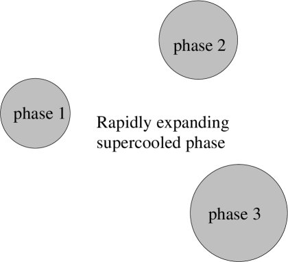
Figure 11: State of the universe

Let us now combine these two facts about the metastable phases of M-theory, and study how the universe will evolve if any region of the universe happens to be in such a metastable phase of M-theory. First of all, due to the cosmological constant term such a region of the universe will expand very rapidly. At the same time in different parts of the universe small regions of more stable phases will form which will then grow, converting the surrounding region of the universe into the more stable phase. In fact inside different bubbles we may have different stable phases of M-theory. In a normal fluid this process will stop when the walls of the expanding bubble eventually collide; and eventually the entire fluid will be converted to the most stable of all the phases. However in the current situation this never happens since the universe as a whole is expanding rapidly due to the cosmological constant. Thus the process continues ad infinitum; the original universe keeps on expanding, and more and more bubbles of stable phases form in different regions of the universe. Eventually every possible phase of M-theory is realized inside one or more bubbles. This situation has been depicted in Fig. 11.

In this picture, no single phase of M-theory is prefered by nature. The world that we see around us exists in a particular phase simply because we happen to live in this part of the world. If we had lived in another part of the world we would see a different phase. Of course, in most of the phases of M-theory life as we know would be impossible, and so nobody would be there to observe these phases. But that is another matter!

6 Summary

There are various aspects of string theory which I have left out of our discussion. These include string theory analysis of black hole entropy, duality between string theory and gauge theory etc. My main focus in this article has been to explain how string theory brings us closer to Einstein’s dream. However we are still quite far from realizing our final goal of finding a complete theory of elementary constituents of matter. It is up to the present and the future generation of string theorists to carry the theory forward towards this goal. It will be an uphill task but worth the effort.

References

- [1] B. Zwiebach, A first course in string theory, Cambridge Univ. Pr. (2004).
- [2] C. V. Johnson, D-branes, Cambridge Univ. Pr. (2003).
- [3] J. Polchinski, String theory. Vol. 1 and 2, Cambridge Univ. Pr. (1998).
- [4] M. B. Green, J. H. Schwarz and E. Witten, Superstring Theory. Vol. 1 and 2, Cambridge Univ. Pr. ( 1987).