Coherence properties of the radiation from X-ray free electron laser

Abstract

We present a comprehensive analysis of coherence properties of the radiation from X-ray free electron laser (XFEL). We consider practically important case when XFEL is optimized for maximum gain. Such an optimization allows to reduce significantly parameter space. Application of similarity techniques to the results of numerical simulations allows to present all output characteristics of the optimized XFEL as functions of the only parameter, ratio of the emittance to the radiation wavelength, $\hat{\epsilon}=2\pi\epsilon/\lambda$. Our studies show that optimum performance of the XFEL in terms of transverse coherence is achieved at the value of the parameter $\hat{\epsilon}$ of about unity. At smaller values of $\hat{\epsilon}$ the degree of transverse coherence is reduced due to strong influence of poor longitudinal coherence on a transverse one. At large values of the emittance the degree of transverse coherence degrades due to poor mode selection. Comparative analysis of existing XFEL projects, European XFEL, LCLS, and SCSS is presented as well.

DEUTSCHES ELEKTRONEN-SYNCHROTRON

in der HELMHOLTZ-GEMEINSCHAFT

DESY 06-137

August 2006

, ,

1 Introduction

Free electron lasing at wavelengths shorter than ultraviolet can be achieved with a single-pass, high-gain FEL amplifier. Because a lack of powerful, coherent seeding sources short-wavelength FEL amplifiers work in so called Self-Amplified Spontaneous Emission (SASE) mode when amplification process starts from shot noise in the electron beam [1, 2, 3]. Present level of accelerator and FEL techniques holds potential for SASE FELs to generate wavelengths as short as 0.1 nm [4, 5, 6].

Experimental realization of X-ray FELs (XFELs) developed very rapidly during last decade. The first demonstration of the SASE FEL mechanism took place in 1997 in the infrared wavelength range [7]. In September of 2000, a group at Argonne National Laboratory (ANL) became the first to demonstrate saturation in a visible (390 nm) SASE FEL [8]. In September 2001, a group at DESY (Hamburg, Germany) has demonstrated lasing to saturation at 98 nm [9, 10]. In June 2006 saturation has been achieved at 13 nm, the shortest wavelength ever generated by FELs. The experimental results have been achieved at FLASH (”F”ree-Electron-”LAS”er in ”H”amburg). Regular user operation of FLASH started in 2005 [11]. Currently FLASH produces GW-level, laser-like VUV radiation pulses with 10 to 50 fs duration in the wavelength range 13-45 nm. After the energy upgrade of the FLASH linac to 1 GeV planned in 2007, it will be possible to generate wavelengths down to 6 nm.

Recently the German government, encouraged by these results, approved funding a hard X-ray SASE FEL user facility – the European X-Ray Free Electron Laser [4]. The US Department of Energy (DOE) has given SLAC the goahead for the engineering design of the Linac Coherent Light Source (LCLS) to be constructed at SLAC [5]. These devices should produce 100 fs X-ray pulses with over 10 to 100 GW of peak power. The main difference between projects is the linear accelerator, an existing room temperature linac for LCLS at SLAC, and future superconducting linac for the European XFEL. The XFEL based on superconducting accelerator technology will make possible not only a jump in a peak brilliance by ten orders of magnitude, but also increase by five orders of magnitude in average brilliance. The LCLS and European XFEL projects are scheduled to start operation in 2009 and 2013, respectively.

In the X-ray FEL the radiation is produced by the electron beam during single-pass of the undulator [1, 2, 3]. The amplification process starts from the shot noise in the electron beam. Any random fluctuations in the beam current correspond to a modulation of the beam current at all frequencies simultaneously. When the electron beam enters the undulator, the presence of the beam modulation at frequencies close to the resonance frequency initiates the process of radiation. The FEL collective instability in the electron beam produces an exponential growth (along the undulator) of the modulation of the electron density on the scale of undulator radiation wavelength. The fluctuations of current density in the electron beam are uncorrelated not only in time but in space, too. Thus, a large number of transverse radiation modes are excited when the electron beam enters the undulator. These radiation modes have different gain. As undulator length progresses, the high gain modes start to predominate more and more. For enough long undulator, the emission will emerge in a high degree of transverse coherence. An intensity gain in excess of $10^{6}-10^{7}$ is obtained in the saturation regime. At this level, the shot noise of the electron beam is amplified up to complete micro-bunching, and all electrons radiate almost in phase producing powerful, coherent radiation.

Understanding of coherence properties of the radiation from SASE FEL is of great practical importance. Properties of the longitudinal coherence have been studied in [12, 13, 14, 15, 16, 17, 18]. It has been found that the coherence time increases first, reaches maximum value in the end of the linear high gain regime and then drops when amplification process enters nonlinear stage [18]. The first analysis of the problem of transverse coherence has been performed in [19]. The problem of start-up from the shot noise has been studied analytically and numerically for the linear stage of amplification. It has been found that the process of formation of transverse coherence is more complicated than that given by naive physical picture of transverse mode selection. Namely, even after finishing the transverse mode selection process the degree of transverse coherence of the radiation from SASE FEL visibly differs from the unity. This is consequence of the interdependence of the longitudinal and transverse coherence. The SASE FEL has poor longitudinal coherence which develops slowly with the undulator length thus preventing a full transverse coherence. First studies of the evolution of transverse coherence in the nonlinear regime of SASE FEL operation have been performed in [20]. It has been found that similarly to the coherence time, the degree of transverse coherence reaches maximum value in the end of the linear regime. Further increase of the undulator length leads to its decrease. Despite output power of the SASE FEL grows continuously in the nonlinear regime, maximum brilliance of the radiation is achieved in the very beginning of the nonlinear regime. Due to a lack of computing power available at that time we limited our study with a specific numerical example just illustrating the general features of coherence properties of the radiation produced by the SASE FEL operating in the nonlinear regime.

In this paper we present general analysis of the coherence properties (longitudinal and transverse) of the radiation from SASE FEL. The results have been obtained with time-dependent, three-dimensional FEL simulation code FAST [21] performing simulation of the FEL process with actual number of electrons in the beam. Using similarity techniques we present universal dependencies for the main characteristics of the SASE FEL covering all practical range of X-ray FELs.

2 Basic relations

Design of the focusing system of XFEL assumes nearly uniform focusing of the electron beam in the undulator, so we consider axisymmetric model of the electron beam. It is assumed that transverse distribution function of the electron beam is Gaussian, so rms transverse size of matched beam is $\sigma=\sqrt{\epsilon\beta}$ ,where $\epsilon=\epsilon_{\mathrm{n}}/\gamma$ is rms beam emittance and $\beta$ is focusing beta-function. An important feature of the parameter space of XFEL is that the space charge field does not influence significantly on the FEL process and calculation of the FEL process can be performed by taking into account diffraction effects, the energy spread in the electron beam, and effects of betatron motion only. In the framework of the three-dimensional theory operation of the FEL amplifier is described by the following parameters: the diffraction parameter $B$, the energy spread parameter $\hat{\Lambda}^{2}_{\mathrm{T}}$, and the betatron motion parameter $\hat{k}_{\beta}$ [22, 23]:

$$B = 2\Gamma\sigma^{2}\omega/c\ ,$$

$$\hat{k}_{\beta} = 1/(\beta\Gamma)\ ,$$

$$\hat{\Lambda}^{2}_{\mathrm{T}} = (\sigma_{\mathrm{E}}/{\mathcal{E}})^{2}/\rho^{2}\ ,$$ (1)

where $\Gamma=\left[I\omega^{2}\theta_{\mathrm{s}}^{2}A_{\mathrm{JJ}}^{2}/(I_{\mathrm{A}}c^{2}\gamma_{\mathrm{z}}^{2}\gamma)\right]^{1/2}$ is the gain parameter and $\rho=c\gamma^{2}_{\mathrm{z}}\Gamma/\omega$ is the efficiency parameter. When describing shot noise in the electron beam, one more parameter appears, the number of electrons on the coherence length, $N_{\mathrm{c}}=I/(e\omega\rho)$. The following notations are used here: $I$ is the beam current, $\omega=2\pi c/\lambda$ is the frequency of the electromagnetic wave, $\theta_{\mathrm{s}}=K_{\mathrm{rms}}/\gamma$, $K_{\mathrm{rms}}$ is the rms undulator parameter, $\gamma$ is relativistic factor, $\gamma^{-2}_{z}=\gamma^{-2}+\theta^{2}_{\mathrm{s}}$, $k_{\mathrm{w}}=2\pi/\lambda_{\mathrm{w}}$ is the undulator wavenumber, $I_{\mathrm{A}}=$ 17 kA is the Alfven current, $A_{\mathrm{JJ}}=1$ for helical undulator and $A_{\mathrm{JJ}}=J_{0}(K_{\mathrm{rms}}^{2}/2(1+K_{\mathrm{rms}}^{2}))-J_{1}(K_{\mathrm{rms}}^{2}/2(1+K_{\mathrm{rms}}^{2}))$ for planar undulator. Here $J_{0}$ and $J_{1}$ are the Bessel functions of the first kind. The energy spread is assumed to be Gaussian with rms deviation $\sigma_{\mathrm{E}}$.

The amplification process in the FEL amplifier passes two stages, linear and nonlinear. The linear stage lasts over significant fraction of the undulator length (about 80%), and the main target for XFEL optimization is the field gain length. In the linear high-gain limit the radiation emitted by the electron beam in the undulator can be represented as a set of modes:

$$E_{\mathrm{x}}+iE_{\mathrm{y}} = \int\mathrm{d}\omega\exp[i\omega(z/c-t)]\times\sum\limits_{n,m}A_{nm}(\omega,z)\Phi_{nm}(r,\omega)\exp[\Lambda_{nm}(\omega)z+in\phi]\ .$$ (2)

When amplification takes place, the mode configuration in the transverse plane remains unchanged while the amplitude grows exponentially with the undulator length. Each mode is characterized by the eigenvalue $\Lambda_{nm}(\omega)$ and the field distribution eigenfunction $\Phi_{nm}(r,\omega)$ in terms of transverse coordinates. At sufficient undulator length fundamental TEM₀₀ mode begins to give main contribution to the total radiation power. Thus, relevant value of interest for XFEL optimization is the field gain length of the fundamental mode, $L_{\mathrm{g}}=1/\mathop{\mathrm{Re}}(\Lambda_{00})$, which gives good estimate for expected length of the undulator needed to reach saturation, $L_{\mathrm{sat}}\simeq 10\times L_{\mathrm{g}}$. Optimization of the field gain length is performed by means of numerical solution of the corresponding eigenvalue equations taking into account all the effects (diffraction, energy spread and emittance) [23, 24]. Computational possibilities of modern computers allows to trace complete parameter space of XFEL (which in fact is 11-dimensional). From practical point of view it is important to find an absolute minimum of the gain length corresponding to optimum focusing beta function. For this practically important case the solution of the eigenvalue equation for the field gain length of the fundamental mode and optimum beta function are rather accurately approximated by [25]:

$$L_{\mathrm{g}} = 1.67\left(\frac{I_{A}}{I}\right)^{1/2}\frac{(\epsilon_{n}\lambda_{\mathrm{w}})^{5/6}}{\lambda^{2/3}}\ \frac{(1+K^{2})^{1/3}}{KA_{JJ}}(1+\delta)\ ,$$

$$\beta_{\mathrm{opt}} \simeq 11.2\left(\frac{I_{A}}{I}\right)^{1/2}\frac{\epsilon_{n}^{3/2}\lambda_{\mathrm{w}}^{1/2}}{\lambda KA_{JJ}}\ (1+8\delta)^{-1/3}\ ,$$

$$\delta = 131\ \frac{I_{A}}{I}\ \frac{\epsilon_{n}^{5/4}}{\lambda^{1/8}\lambda_{\mathrm{w}}^{9/8}}\ \frac{\sigma_{\gamma}^{2}}{(KA_{JJ})^{2}(1+K^{2})^{1/8}}\ ,$$ (3)

where $\sigma_{\gamma}=\sigma_{\mathrm{E}}/m_{\mathrm{e}}c^{2}$. Accuracy of this fit is better than 5% in the range of parameter $\hat{\epsilon}=2\pi\epsilon/\lambda$ from 1 to 5.

Equation (3) demonstrates clear interdependence of physical parameters defining operation of the XFEL. Let us consider the case of negligibly small energy spread. Under this condition diffraction parameter $B$ and parameter of betatron oscillations, $\hat{k}_{\beta}$ are functions of the only parameter $\hat{\epsilon}$:

$$B\simeq 12.5\times\hat{\epsilon}^{5/2}\ ,\qquad\hat{k}_{\beta}=1/(\beta\Gamma)\simeq 0.158\times\hat{\epsilon}^{3/2}\ .$$ (4)

FEL equations written down in the dimensionless form involve an additional parameter $N_{\mathrm{c}}$ defining the initial conditions for the start-up from the shot noise. Note that the dependence of output characteristics of the SASE FEL operating in saturation is slow, in fact logarithmic in terms of $N_{\mathrm{c}}$. Thus, we can conclude that with logarithmic accuracy in terms of $N_{\mathrm{c}}$, characteristics of the SASE FEL written down in a normalized form are functions of the only parameter $\hat{\epsilon}$.

3 An approach for numerical simulations

Rigorous studies of the nonlinear stage of amplification is possible only with numerical simulation code. Typically FEL codes use an artificial ensemble of macroparticles for simulating the FEL process when one macroparticle represents large number of real electrons. Thus, a natural question arises if macroparticle phase space distributions are identical to those of actual electron beam at all stages of amplification. Let us trace typical procedure for preparation of an artificial ensemble [26, 27]. The first step of particle loading consists in a quasi-uniform distribution of the macroparticles in the phase space. At this stage an ensemble of particles with random distribution is generated which occupies a fraction of the phase space. Then this ensemble is copied on the other parts of the phase space to provide pseudo-uniform loading of the phase space. Pseudo-uniformity means that initial microbunching at the fundamental harmonic (or for several harmonics) is equal to zero. Also, phase positions of the mirrored particles are correlated such that microbunching does not appear due to betatron oscillations, or due to the energy spread. Finally, artificial displacements of the macroparticles are applied to provide desired (in our case gaussian) statistics of microbunching at the undulator entrance. We note that it is not evident that such an artificial ensemble reflects actual physical situation for a short wavelength SASE FEL. Let us consider an example of the SASE FEL operating at the radiation wavelength of 0.1 nm. With the peak current of 5 kA we find that the number of electrons per wavelength is about $10^{4}$. On the other hand, it is well known that properties of an artificial ensemble (even at the first step of pseudo-uniform loading) converge very slowly to the model of continuous media. In fact, even with the number of macroparticles per radiation wavelength $6.4\times 10^{4}$ the FEL gain still visibly deviates from the target value. Introducing of an artificial noise makes situation with the quality of an ensemble preparation even more problematic. The only way to test the quality of an artificial ensemble is to perform numerical simulations with actual number of electrons in the beam. We constructed such a version of three-dimensional, time-dependent FEL simulation code FAST [21]. Comparison of the results with direct simulations of the electron beam and with an artificial distributions has shown that artificial ensembles are not adequate to the problem. Artificial effects are pronouncing especially when calculating such fine features as transverse correlation functions. Thus, all the simulations presented in this paper have been performed with code FAST using actual number of electrons in the beam.

4 General overview of the properties of the radiation form SASE FEL

The result of each simulation run contains an array of complex amplitudes $\tilde{E}$ for electromagnetic fields on a three-dimensional mesh. At the next stage of the numerical experiment the data arrays are handled with postprocessor codes to calculate different characteristics of the radiation. However, as the first step it is worthwhile to obtain qualitative analysis of the object under study. The plots in an upper row of Fig. 1 show evolution of the power density distribution, $I=|\tilde{E}|^{2}$, in a slice of the radiation pulse along the undulator. We see that due to the start-up of amplification process from the shot noise many transverse radiation modes are excited when electron beam enters the undulator. Mode selection process (2) serves as a filter for selection of the fundamental radiation mode having maximum gain.

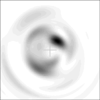
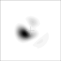
Figure 1: Evolution of the power density distribution in a slice (top) and normalized power in a radiation pulse (bottom) versus $\hat{s}=\rho\omega_{0}(z/\bar{v}_{z}-t)$ for the reduced lengths $\hat{z}=18.4$, 31.6, and 44.8 (left, middle, and right plots, respectively). Here $\hat{\epsilon}=2$. Crosses show geometrical center of the radiation beam.

Figure 2: Averaged normalized efficiency, $\hat{\eta}$, and normalized rms deviation of instantaneous radiation power, $\sigma_{\mathrm{P}}$ along the normalized undulator length, $\hat{z}=\Gamma z$. Here $\hat{\epsilon}=2$.

Figure 3: Right plot: normalized coherence time $\hat{\tau}_{\mathrm{c}}$, along the normalized undulator length, $\hat{z}=\Gamma z$. Left plot: degree of transverse coherence, $\zeta$ (solid line), and normalized degeneracy parameter of the radiation, $\hat{\delta}$ (dashed line), along the normalized undulator length, $\Gamma z$. Dotted line shows $\sigma_{\mathrm{P}}^{2}$ (see Fig. 3). Here $\hat{\epsilon}=2$.

Integration of the power density over transverse cross section of the photon beam gives us instantaneous radiation power, $P\propto\int I\mathop{\mathrm{d}}\vec{r}_{\perp}$. Evolution of temporal structure of the radiation power along the undulator is traced in Fig. 1 in terms of normalized radiation power $\hat{\eta}=P/(\rho P_{\mathrm{b}})$ where $P_{\mathrm{b}}=\gamma mc^{2}I/e$ is the electron beam power. Averaging of the radiation power along the pulse gives us averaged radiation power. Evolution of normalized averaged power $\langle\hat{\eta}\rangle$ along normalized undulator length $\hat{z}=\Gamma z$ is shown in Fig. 3. Note that the radiation produced by SASE FEL operating in the linear regime holds properties of completely chaotic polarized light [18] – a statistical object well described in the framework of statistical optics [28]. This is simple consequence of the fact that the shot noise in the electron beam is a Gaussian random process. The FEL amplifier, operating in the linear regime, can be considered as a linear filter which does not change the statistics of the signal. As a result, we can define general statistical properties of the output radiation without any calculations. For instance, in the case of the SASE FEL the real and imaginary parts of the slowly varying complex amplitudes of the electric field of the electromagnetic wave, $\tilde{E}$ , have a Gaussian distribution, the instantaneous power density, $I=|\tilde{E}|^{2}$, fluctuates in accordance with the negative exponential distribution (see Fig. 4):

$$p(I)=\frac{1}{\langle I\rangle}\exp\left(-\frac{I}{\langle I\rangle}\right)\ .$$ (5)

Due to the start-up of amplification process from the shot noise many transverse radiation modes are excited when electron beam enters the undulator. For gaussian random process any integral of the power density, for example, radiation power $P$, fluctuates in accordance with the gamma distribution:

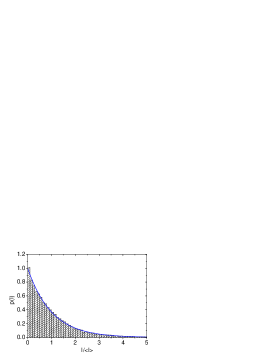
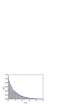
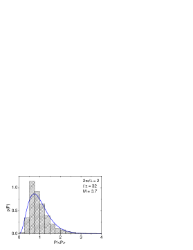
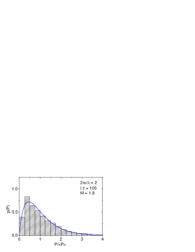
Figure 4: Probability density distributions of the instantaneous power density $I=|\tilde{E}|^{2}$ (top), and of the instantaneous radiation power $P$ (bottom) from SASE FEL for different stages of amplification: linear regime ($\hat{z}=32)$, saturation regime ($\hat{z}=63)$, and deep nonlinear regime ($\hat{z}=105$). Solid lines on the power density histograms (top) represent negative exponential distribution (5). Solid lines on power histograms (bottom) represent gamma distribution (6) with $M=1/\sigma_{\mathrm{P}}^{2}$ (see Fig. 3). Here $\hat{\epsilon}=2$.

$$p({P})=\frac{M^{M}}{\Gamma(M)}\left(\frac{P}{\langle P\rangle}\right)^{M-1}\frac{1}{\langle P\rangle}\exp\left(-M\frac{P}{\langle P\rangle}\right)\ ,$$ (6)

where $\Gamma(M)$ is the gamma function with argument $M$, and

$$M=\frac{1}{\sigma_{\mathrm{P}}^{2}}\ ,$$ (7)

and $\sigma_{\mathrm{P}}^{2}=\langle(P-\langle P\rangle)^{2}\rangle/\langle P\rangle^{2}$ is the relative dispersion of the radiation power. Note that for completely chaotic polarized light parameter $M$ has clear physical interpretation, it is the number of modes [22]. Thus, it becomes clear that the relative dispersion of the radiation power directly relates to the coherence properties of the SASE FEL operating in the linear regime. The degree of transverse coherence in this case can be naturally defined as:

$$\zeta=\frac{1}{M}=\sigma^{2}_{\mathrm{P}}\ .$$ (8)

Indeed, in the linear regime we deal with a Gaussian random process, and the power density fluctuates in accordance with the negative exponential distribution and its relative width is equal to 1. If there is full transverse coherence then the same refers to the power. If the radiation is partially coherent, then we have a more general law for power fluctuations, namely the gamma distribution (6). In the linear regime fluctuations of the radiation power, $\sigma_{\mathrm{P}}$, grow steadily with the undulator length (see Fig. 3) because of mode selection process (2).

Figure 5: Diffraction parameter $B$ versus parameter $\hat{\epsilon}$ for optimized XFEL.

Another physical parameter of the problem relating to the transverse coherence is diffraction parameter $B$. Mechanism of formation of transverse coherence is rather transparent. If diffraction expansion of the radiation on a scale of the field gain length is comparable with the transverse size of the electron beam, we can expect a high degree of transverse coherence. For this range of parameters the value of the diffraction parameter is small. If diffraction expansion of the radiation is small (which happens at large values of the diffraction parameter) then we can expect significant degradation of the degree of transverse coherence. This happens simply because different parts of the beam produce radiation nearly independently. In terms of the radiation expansion in the eigenmodes (2) this range of parameters corresponds to degeneration of modes (see Appendix A). Diffraction parameter for optimized XFEL exhibits strong dependence on the parameter $\hat{\epsilon}$ (see eq. (4) and Fig. 5), and we can expect that the degree of transverse coherence should drop rapidly with the increase of the parameter $\hat{\epsilon}$.

An important physical quantity describing random fields is the coherence time. Figure 1 gives qualitative picture of formation of longitudinal coherence in SASE FEL. At the beginning of the undulator the radiation is simply incoherent undulator radiation. When amplification process starts to dominate over spontaneous emission, we obtain formation of spikes (wavepackets). The width of the spikes defines the coherence time. In the high gain linear regime the width of spikes grows with the undulator length, and the coherence time also grows proportionally to the square root of the undulator length. It achieves maximum value in the end of linear regime and then decreases rapidly in the nonlinear regime (see Fig. 3). The maximum value of the coherence time depends on the saturation length and, therefore, on the value of the parameter $N_{\mathrm{c}}$ [18].

We see that physical background defining general features of the radiation from SASE FEL operating in the linear regime is rather transparent. Despite the behavior of the SASE FEL in the nonlinear regime is rather complicated (see Figs. 3 and 3), we will show below that the main characteristics of the SASE FEL operating at the saturation point have rather simple physical scaling.

5 General definitions

5.1 Degree of transverse coherence

The transverse coherence properties of the radiation are described in terms of the transverse correlation functions. The first-order transverse correlation function is defined as

$$\gamma_{1}(\vec{r}_{\perp},\vec{r}\prime_{\perp},z,t)=\frac{\langle\tilde{E}(\vec{r}_{\perp},z,t)\tilde{E}^{*}(\vec{r}\prime_{\perp},z,t)\rangle}{\left[\langle|\tilde{E}(\vec{r}_{\perp},z,t)|^{2}\rangle\langle|\tilde{E}(\vec{r}\prime_{\perp},z,t)|^{2}\rangle\right]^{1/2}}\ ,$$

where $\tilde{E}$ is the slowly varying amplitude of the amplified wave:

$$E=\tilde{E}(\vec{r}_{\perp},z,t)\mathrm{e}^{\mathop{\mathrm{i}}\omega_{0}(z/c-t)}+{\mathrm{C.C.}}\ .$$ (9)

In the following we consider the model of a stationary random process, thus assuming that $\gamma_{1}$ does not depend on time. We define the degree of transverse coherence as:

$$\zeta=\frac{\int|\gamma_{1}(\vec{r}_{\perp},\vec{r}\prime_{\perp})|^{2}I(\vec{r}_{\perp})I(\vec{r}\prime_{\perp})\mathop{\mathrm{d}}\vec{r}_{\perp}\mathop{\mathrm{d}}\vec{r}\prime_{\perp}}{[\int I(\vec{r}_{\perp})\mathop{\mathrm{d}}\vec{r}_{\perp}]^{2}}\ .$$ (10)

When SASE FEL operates in the linear regime such a definition for the degree of transverse coherence is mathematically equivalent to (8) expressed in terms of the relative dispersion of the instantaneous radiation power, $\sigma_{\mathrm{P}}^{2}$. Analysis of the asymptotic of the deep nonlinear regime (see Fig. 3) shows that surprisingly the degree of transverse coherence defined by (10) again tends to be an agreement with (8). This feature has deep physical background. When amplification process just enters nonlinear stage, the statistics of the radiation is not Gaussian anymore. In particular, the probability distribution function of the radiation power density, is not negative exponential distribution (see Fig. 4). Thus, definition of the degree of transverse coherence (8) has no physical sense near the saturation point. However, simulations show that in the deep nonlinear regime the probability distribution of the radiation power density again tends to the negative exponential distribution. This gives us a hint that the properties of the radiation from SASE FEL operating in the deep nonlinear regime tend again to be the properties of completely chaotic polarized light. Similar asymptotical behavior has been observed in the framework of the one-dimensional model as well [18].

5.2 Coherence time

Longitudinal coherence is described in terms of time correlation functions. The first order time correlation function, $g_{1}(t,t^{\prime})$, is calculated in accordance with the definition:

$$g_{1}(\vec{r},t-t^{\prime})=\frac{\langle\tilde{E}(\vec{r},t)\tilde{E}^{*}(\vec{r},t^{\prime})\rangle}{\left[\langle\mid\tilde{E}(\vec{r},t)\mid^{2}\rangle\langle\mid\tilde{E}(\vec{r},t^{\prime})\mid^{2}\rangle\right]^{1/2}}\ ,$$ (11)

For a stationary random process time correlation functions are functions of the only argument, $\tau=t-t^{\prime}$. The coherence time is defined as [22]:

$$\tau_{\mathrm{c}}=\int\limits^{\infty}_{-\infty}|g_{1}(\tau)|^{2}\mathop{\mathrm{d}}\tau\ .$$ (12)

5.3 Brilliance and degeneracy parameter

Main figure of merit of the SASE FEL performance is brilliance, i.e. density of photons in the phase space. In fact, the brilliance is proportional to the degeneracy parameter $\delta$, i.e. the number of photons per mode (coherent state). Note that when $\delta\gg 1$, the classical statistics is applicable, while quantum description of the field is necessary as soon as $\delta$ is comparable to (or less than) one. Using the definitions of the degree of transverse coherence (10) and coherence time (12), one can define degeneracy parameter:

$$\delta=\dot{N}_{ph}\tau_{\mathrm{c}}\zeta\ ,$$ (13)

where $\dot{N}_{ph}=N_{ph}^{tot}/T$ is the photon flux, $N_{ph}^{tot}$ is the total number of photons in a long flat-top pulse of duration $T$ (as everywhere in this paper we consider ensemble average values). The definition (13) is perfect for a Gaussian random process (that we have in linear regime). Indeed, degree of transverse coherence is an inverse number of transverse modes (8), while $\tau_{\mathrm{c}}/T$ is an inverse number of longitudinal modes within the pulse [22, 28]. Thus, degeneracy parameter is equal to the number of photons per pulse divided by total number of modes per pulse (that is equal to the squared inverse rms fluctuations of pulse energy [22]). It can be directly measured in an experiment for SASE FEL operating in the linear regime. We use (13) as a natural generalization to characterize SASE FEL properties at saturation.

Let us introduce a notion of normalized degeneracy parameter

$$\hat{\delta}=\hat{\eta}\hat{\tau}_{\mathrm{c}}\zeta\ .$$ (14)

Here normalized FEL efficiency is defined as $\hat{\eta}=P/(\rho P_{\mathrm{b}})$ where $P$ is radiation power, and $P_{\mathrm{b}}=\gamma mc^{2}I/e$ is electron beam power. Normalized coherence time is defined as $\hat{\tau}_{\mathrm{c}}=\rho\omega\tau_{\mathrm{c}}$. Parameter $\hat{\delta}$ and the degeneracy parameter $\delta$ are simply related as:

$$\delta=\frac{P_{\mathrm{b}}}{\hbar\omega^{2}}\hat{\delta}\ ,$$ (15)

or, in practical units

$$\delta\simeq 2.7\times 10^{7}\times\lambda^{2}[\mathrm{\AA}\ ]\times I[\mathrm{kA}]\times E[\mathrm{GeV}]\times\hat{\delta}\ ,$$ (16)

where $E=\gamma mc^{2}$ is the electron energy. Note that the degeneracy parameter is very large even for a SASE FEL operating at the wavelength of 0.1 nm. With multi-kA electron beams and other relevant parameters, mentioned in Table 1, degeneracy parameter would be of the order of $10^{8}$ - $10^{9}$. Thus, a classical treatment of SASE FEL is justified.

Let us now turn to the calculation of peak brilliance. It is defined as a transversely coherent spectral flux:

$$B_{r}=\frac{\omega\mathop{\mathrm{d}}\dot{N}_{ph}}{\mathop{\mathrm{d}}\omega}\ \frac{\zeta}{\left(\frac{\lambda}{2}\right)^{2}}\ .$$ (17)

The spectrum of SASE FEL radiation in a high-gain linear regime has a Gaussian shape, it is also close to the Gaussian at saturation point [22]. In this case

$$\frac{\omega\mathop{\mathrm{d}}\dot{N}_{ph}}{\mathop{\mathrm{d}}\omega}=\frac{\omega\dot{N}_{ph}}{\sqrt{2\pi}\sigma_{\omega}}\ ,$$

where $\sigma_{\omega}$ is the rms bandwidth. For a Gaussian line, with the definition of coherence time (12), one gets [22]:

$$\tau_{\mathrm{c}}=\frac{\sqrt{\pi}}{\sigma_{\omega}}\ .$$

Thus, it follows from (14) and (17) that

$$B_{r}=\frac{4\sqrt{2}c}{\lambda^{3}}\ \delta\ .$$ (18)

The peak brilliance can then be calculated as follows

$$B_{r}[\mathrm{phot./(sec.\ mrad^{2}\ mm^{2}\ 0.1\%\ bandw.)}]\simeq 4.5\times 10^{31}\times\frac{I[\mathrm{kA}]\times E[\mathrm{GeV}]}{\lambda[\mathrm{\AA}\ ]}\times\hat{\delta}\ .$$ (19)

For future SASE FELs, operating at 1 Å , an expected value of the peak brilliance is $10^{32}$-$10^{33}$.

An important feature of our analysis is application of similarity techniques to the analysis of simulation results which allows to derive universal parametric dependencies of the output characteristics of the radiation. As we mentioned above, within accepted approximations (optimized SASE FEL and negligibly small energy spread in the electron beam), output characteristics of SASE FEL are universal functions of two parameters, normalized undulator length $\hat{z}=\Gamma z$ and parameter $\hat{\epsilon}$. If one traces evolution of the brilliance (or, degeneracy parameter) of the radiation along the undulator length there is always the point, which we define as the saturation point, where the brilliance reaches maximum value (see Fig. 3). In the following we present characteristics of the radiation at the saturation point which are universal functions of the only parameter $\hat{\epsilon}$.

6 Properties of the radiation from optimized XFEL operating in the saturation regime

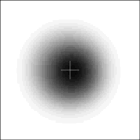
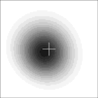
Figure 6: Top: normalized power in a radiation pulse, $\hat{\eta}$ versus $\hat{s}=\rho\omega(z/\bar{v}_{z}-t)$. Bottom: typical power density distribution in a slice of the radiation. SASE FEL operates in the saturation. Values of $\hat{\epsilon}=1$, 2 and 4.5 correspond to the left, middle, and right plot, respectively. Crosses show geometrical center of the beam.

Figure 7: Saturation length $\hat{z}_{\mathrm{sat}}=\Gamma z_{\mathrm{sat}}$ versus parameter $\hat{\epsilon}$.

Figure 8: Degree of transverse coherence, $\zeta_{\mathrm{sat}}$, and normalized coherence time, $\hat{\tau}_{\mathrm{c}}^{\mathrm{sat}}$ in the saturation versus parameter $\hat{\epsilon}$.

Figure 9: Averaged efficiency, $\langle\hat{\eta}_{\mathrm{sat}}\rangle$, and normalized degeneracy parameter, $\hat{\delta}_{\mathrm{sat}}$, in the saturation versus parameter $\hat{\epsilon}$.

Simulations of the FEL process have been performed for the case of a long bunch with uniform axial profile of the beam current. Such a model provides rather accurate predictions for the coherence properties of the XFEL, since typical radiation pulse from the XFEL is much longer than the coherence time. Calculations has been performed with FEL simulation code FAST using actual number of electrons in the beam. The value of parameter $N_{\mathrm{c}}=8\times 10^{5}$ corresponds to the parameter range of XFEL operating at the radiation wavelength about 0.1 nm.

Figure 6 gives visual picture of the slice properties of the radiation at the saturation for different values of the parameter $\hat{\epsilon}$. Saturation point is defined as the point where the radiation achieves maximum brilliance (or, maximum degeneracy parameter (14)). A series of simulation runs has been performed in the range of the parameter $\hat{\epsilon}=0.25\ldots 4.5$. Application of similarity techniques described above allowed us to extract universal parametric dependencies of the main characteristics of the optimized XFEL operating in the saturation regime (see Figs. 9-9).

Figure 9 shows the dependence of the saturation length $\hat{z}_{\mathrm{sat}}=\Gamma z_{\mathrm{sat}}$ on parameter $\hat{\epsilon}$. Analysis of the curve shows that the saturation length scales as $\hat{z}_{\mathrm{sat}}\propto\hat{\epsilon}^{5/6}$. Such dependence directly follows from the optimization procedure of the gain length given by (3). The normalized coherence time in the saturation regime, $\hat{\tau}_{\mathrm{c}}^{\mathrm{sat}}$ is also proportional to $\hat{\epsilon}^{5/6}$ (see Fig. 9).

Figure 10: Partial contributions of the modes with azimuthal index $m=0\ldots 4$ into the total power versus parameter $\hat{\epsilon}$. SASE FEL operates in the saturation.

The dependence of the degree of transverse coherence in the saturation regime on the parameter $\hat{\epsilon}$ exhibits rather complicated behavior (see Fig. 9). It reaches maximum value in the range of $\hat{\epsilon}$ values about of unity, and drops at small and large values of $\hat{\epsilon}$. Actually, the degree of transverse coherence is formed due to two effects. The first effect takes place due to interdependence of the poor longitudinal coherence and transverse coherence [19]. Due to the start-up from shot noise every radiation mode entering (2) is excited within finite spectral bandwidth. This means that in the high gain linear regime the radiation of the SASE FEL is formed by many fundamental TEM₀₀ modes with different frequencies. The transverse distribution of the radiation field of the mode is also different for different frequencies. Smaller value of the diffraction parameter (i.e. smaller value of $\hat{\epsilon}$) corresponds to larger deviation of the radiation mode from the plane wave. This explains a decrease of the transverse coherence at small values of $\hat{\epsilon}$. When the parameter $\hat{\epsilon}$ increases, the diffraction parameter increases as well thus leading to the degeneration of the radiation modes. Amplification process in the SASE FEL passes limited number of the field gain lengths, and starting from some value of $\hat{\epsilon}$ the linear stage of amplification becomes too short to provide mode selection process (2). When amplification process enters nonlinear stage, the mode content of the radiation becomes even more rich due to independent growth of the radiation modes in the nonlinear medium (see Fig. 10). Thus, at large values of $\hat{\epsilon}$ the degree of transverse coherence is limited by poor mode selection. Analytical estimations, presented in Appendix A, show that in the limit of large emittance, $\hat{\epsilon}\gg 1$, the degree of transverse coherence scales as $1/\hat{\epsilon}^{2}$.

We present in Fig. 9 the plots for normalized efficiency and degeneracy parameter for optimized XFEL. Normalized efficiency in saturation has simple scaling, it falls inversely proportional to the parameter $\hat{\epsilon}$. Taking into account that the value of the coherence time $\hat{\tau}_{\mathrm{c}}^{\mathrm{sat}}$ scales proportional to $\hat{\epsilon}^{5/6}$, we find that the normalized degeneracy parameter of the radiation is nearly proportional to the degree of transverse coherence, $\hat{\delta}_{\mathrm{sat}}\propto\zeta/\hat{\epsilon}^{1/6}$.

Table 1: Parameter space of XFEL projects

	European XFEL		LCLS	SCSS
	SASE1	SASE2
Radiation wavelength, nm	0.1	0.15	0.15	0.1
Beam energy, GeV	17.5	17.5	14.35	6.135
rms normalized emittance $\epsilon_{n}$, mm-mrad	1.4	1.4	1.2	0.85
Parameter $\hat{\epsilon}$	2.6	1.7	1.8	4.5
Degree of transverse coherence $\zeta$	0.65	0.85	0.83	0.24

Finally, in Table 1 we present comparison of existing XFEL projects, the European XFEL, LCLS and SCSS in terms of degree of transverse coherence [4, 5, 6]. We see that the European XFEL and LCLS are in the same range of parameter space. These projects assume conservative value of the emittance, and relatively high degree of transverse coherence is achieved by increasing the energy of the driving accelerator. Project SCSS assumes much smaller energy of the driving accelerator. Thus, despite much smaller value of the normalized emittance it falls in the range of parameters for the output radiation with poor transverse coherence.

Appendix A Solution of the eigenvalue equation and estimates of transverse coherence in the limit of wide electron beam

A.1 Basic equation

Let us have at the undulator entrance a continuous electron beam with the current $I_{0}$, with the Gaussian distribution in energy

$$F({\mathcal{E}}-{\mathcal{E}}_{0})=\left(2\pi\langle(\Delta{\mathcal{E}})^{2}\rangle\right)^{-1/2}\exp\left(-\frac{({\mathcal{E}}-{\mathcal{E}}_{0})^{2}}{2\langle(\Delta{\mathcal{E}})^{2}\rangle}\right)\ ,$$ (A.1)

and in a transverse phase plane

$$f(x,x^{\prime})=(2\pi\sigma^{2}k_{\beta})^{-1}\exp\left[-\frac{x^{2}+(x^{\prime})^{2}/k_{\beta}^{2}}{2\sigma^{2}}\right]\ ,$$ (A.2)

the same in $y$ phase plane. Here $k_{\beta}=1/\beta$ is the wavenumber of betatron oscillations and $\sigma=\sqrt{\epsilon\beta}$.

The results of this paper can be used in the case of superposition of the natural undulator focusing and an alternating-gradient external focusing if the following condition is satisfied [23]:

$$\frac{L_{f}}{2\pi\beta}\ll\min\left(1,\frac{\lambda}{2\pi\epsilon}\right)\ ,$$

where $L_{f}$ is a period of the external focusing structure, $\beta$ is an average beta-function, $\epsilon$ is rms emittance of an electron beam, and $\lambda$ is a radiation wavelength. This condition is met in many practical situations.

Using cylindrical coordinates, in the high-gain limit we seek the solution for a slowly varying complex amplitude of the electric field of the electromagnetic wave in the form [22]:

$$\tilde{E}(z,r,\varphi)=\Phi_{nm}(r)\exp(\Lambda z)\left(\begin{array}[]{c}\sin(n\varphi)\\ \cos(n\varphi)\end{array}\right)\ ,$$ (A.3)

where $n$ is an integer, $n\geq 0$. For each $n$ there are many radial eigenmodes that differ by eigenvalue $\Lambda$ and eigenfunction $\Phi_{nm}(r)$. The integro-differential equation for radiation field eigenmodes [24, 31, 32] taking into account the space charge effect [23] can be written in the following normalized form:

$$\left[\frac{\mathop{\mathrm{d}}^{2}}{\mathop{\mathrm{d}}\hat{r}^{2}}+\frac{1}{\hat{r}}\frac{\mathop{\mathrm{d}}}{\mathop{\mathrm{d}}\hat{r}}-\frac{n^{2}}{\hat{r}^{2}}+2\mathop{\mathrm{i}}B\hat{\Lambda}\right]\Phi_{nm}(\hat{r})=-4\int\limits^{\infty}_{0}\mathop{\mathrm{d}}\hat{r}^{\prime}\hat{r}^{\prime}\left\{\Phi_{nm}(\hat{r}^{\prime})\right.$$

$$\left.+\frac{\hat{\Lambda}^{2}_{\mathrm{p}}}{2}\left[\frac{\mathop{\mathrm{d}}^{2}}{\mathop{\mathrm{d}}\hat{r}^{\prime 2}}+\frac{1}{\hat{r}^{\prime}}\frac{\mathop{\mathrm{d}}}{\mathop{\mathrm{d}}\hat{r}^{\prime}}-\frac{n^{2}}{\hat{r}^{\prime 2}}+2\mathop{\mathrm{i}}B\hat{\Lambda}\right]\Phi_{n}(\hat{r}^{\prime})\right\}$$

$$\times\int\limits^{\infty}_{0}\mathop{\mathrm{d}}\zeta\frac{\zeta}{\sin^{2}(\hat{k}_{\beta}\zeta)}\exp\left[-\frac{\hat{\Lambda}^{2}_{\mathrm{T}}\zeta^{2}}{2}-(\hat{\Lambda}+\mathop{\mathrm{i}}\hat{C})\zeta\right]$$

$$\times\exp\left[-\frac{(1-\mathop{\mathrm{i}}B\hat{k}_{\beta}^{2}\zeta/2)(\hat{r}^{2}+\hat{r}^{\prime 2})}{\sin^{2}(\hat{k}_{\beta}\zeta)}\right]$$

$$\times I_{n}\left[\frac{2(1-\mathop{\mathrm{i}}B\hat{k}_{\beta}^{2}\zeta/2)\hat{r}\hat{r}^{\prime}\cos(\hat{k}_{\beta}\zeta)}{\sin^{2}(\hat{k}_{\beta}\zeta)}\right]\ ,$$ (A.4)

where $I_{n}$ is the modified Bessel function of the first kind. The following notations are used here: $\hat{r}=r/(\sigma\sqrt{2})$, $B=2\sigma^{2}\Gamma\omega/c$ is the diffraction parameter, $\hat{k}_{\beta}=k_{\beta}/\Gamma$ is the betatron motion parameter, $\hat{\Lambda}^{2}_{\mathrm{p}}=2c^{2}(A_{\mathrm{JJ}}\theta_{\mathrm{s}}\sigma\omega)^{-2}$ is the space charge parameter, $\hat{\Lambda}^{2}_{\mathrm{T}}=\langle(\Delta{\mathcal{E}})^{2}\rangle/(\rho^{2}{\mathcal{E}}^{2})$ is the energy spread parameter, $\hat{C}=\left[k_{\mathrm{w}}-\omega/(2c\gamma_{z}^{2})\right]/\Gamma$ is the detuning parameter, $\Gamma=\left[A_{\mathrm{JJ}}^{2}I_{0}\omega^{2}\theta^{2}_{\mathrm{s}}\left(I_{\mathrm{A}}c^{2}\gamma^{2}_{z}\gamma\right)^{-1}\right]^{1/2}$ is the gain parameter, $\rho=c\gamma_{z}^{2}\Gamma/\omega$ is the efficiency parameter, $\omega$ is the frequency of the electromagnetic wave, $\theta_{\mathrm{s}}=K_{\mathrm{rms}}/\gamma$, $K_{\mathrm{rms}}$ is the rms undulator parameter, $\gamma$ is relativistic factor, $\gamma^{-2}_{z}=\gamma^{-2}+\theta^{2}_{\mathrm{s}}$, $k_{\mathrm{w}}$ is the undulator wavenumber, $I_{\mathrm{A}}=$ 17 kA is the Alfven current, $A_{\mathrm{JJ}}=1$ for helical undulator and $A_{\mathrm{JJ}}=J_{0}(K_{\mathrm{rms}}^{2}/2(1+K_{\mathrm{rms}}^{2}))-J_{1}(K_{\mathrm{rms}}^{2}/2(1+K_{\mathrm{rms}}^{2}))$ for planar undulator. Here $J_{0}$ and $J_{1}$ are the Bessel functions of the first kind. The space charge effect is included into (A.4) under the condition $\sigma^{2}\gg c^{2}\gamma^{2}_{z}/\omega^{2}$.

A.2 Exact solution

As suggested in [24] we apply to (A.4) the Hankel transformation defined by the following transform pair:

$$\bar{\Phi}_{nm}(p)=\int\limits^{\infty}_{0}\mathop{\mathrm{d}}\hat{r}\hat{r}J_{n}(p\hat{r})\Phi_{nm}(\hat{r})\ ,\qquad\Phi_{nm}(\hat{r})=\int\limits^{\infty}_{0}\mathop{\mathrm{d}}ppJ_{n}(p\hat{r})\bar{\Phi}_{nm}(p)\ .$$

Then we obtain the integral equation for the Hankel transform $\bar{\Phi}_{nm}(p)$ [23]:

$$\bar{\Phi}_{nm}(p) = -\frac{1}{2\mathop{\mathrm{i}}B\hat{\Lambda}-p^{2}}\int\limits^{\infty}_{0}\mathop{\mathrm{d}}p^{\prime}p^{\prime}\bar{\Phi}_{nm}(p^{\prime})\left[1+\frac{\hat{\Lambda}^{2}_{\mathrm{p}}(2\mathop{\mathrm{i}}B\hat{\Lambda}-p^{\prime 2})}{2}\right]$$ (A.5)

$$\times \int\limits^{\infty}_{0}\mathop{\mathrm{d}}\zeta\frac{\zeta}{(1-\mathop{\mathrm{i}}B\hat{k}_{\beta}^{2}\zeta/2)^{2}}\exp\left[-\frac{\hat{\Lambda}^{2}_{\mathrm{T}}\zeta^{2}}{2}-(\hat{\Lambda}+\mathop{\mathrm{i}}\hat{C})\zeta\right]$$

$$\times \exp\left[-\frac{p^{2}+p^{\prime 2}}{4(1-\mathop{\mathrm{i}}B\hat{k}_{\beta}^{2}\zeta/2)}\right]I_{n}\left[\frac{pp^{\prime}\cos(\hat{k}_{\beta}\zeta)}{2(1-\mathop{\mathrm{i}}B\hat{k}_{\beta}^{2}\zeta/2)}\right]\ .$$

When the space charge field is negligible, $\hat{\Lambda}^{2}_{\mathrm{p}}\to 0$, this equation is reduced to that derived in [24].

To solve (A.5) we discretize it:

$$p_{i}=\Delta(i-\frac{1}{2})\ ,\qquad i=1,2,...,K\ ,$$

$$p^{\prime}_{j}=\Delta(j-\frac{1}{2})\ ,\qquad j=1,2,...,K\ ,$$

where $\Delta$ and $K$ should be chosen such that the required accuracy is provided. Then we obtain a matrix equation

$$\bar{\Phi}_{nm}(i)=M_{n}(i,j)\bar{\Phi}_{nm}(j)\ ,$$

or, $[M_{n}-I]\bar{\Phi}_{nm}=0$, where $I$ is a unit matrix. Matrix $M_{n}$ depends on an eigenvalue $\hat{\Lambda}$ as well as on the problem parameters: $B$, $\hat{k}_{\beta}$, $\hat{\Lambda}^{2}_{\mathrm{T}}$, $\hat{\Lambda}^{2}_{\mathrm{p}}$, and $\hat{C}$. The eigenvalues of all radial modes for a given azimuthal index $n$ can be found by solving the equation $|M_{n}-I|=0$. Then the calculation of the eigenmodes is straightforward.

This algorithm allows one to find with any desirable accuracy the eigenvalues and eigenfunctions of a high-gain FEL including all the important effects: diffraction, betatron motion, energy spread, space charge, and frequency detuning. Therefore, it can be considered as a universal tool for calculation and optimization of high-gain FELs of wavelength range from infrared to X-ray.

A.3 Parallel cold beam, large diffraction parameter

A parallel beam limit is the case when there is no betatron motion, i.e. $\hat{k}_{\beta}\to 0$. Let us also assume here for the sake of compactness that the effects of energy spread and space charge can be neglected ($\hat{\Lambda}^{2}_{\mathrm{T}}\to 0$, $\hat{\Lambda}^{2}_{\mathrm{p}}\to 0$). Equation (A.4) can then be reduced to

$$\left[\frac{\mathop{\mathrm{d}}^{2}}{\mathop{\mathrm{d}}\hat{r}^{2}}+\frac{1}{\hat{r}}\frac{\mathop{\mathrm{d}}}{\mathop{\mathrm{d}}\hat{r}}-\frac{n^{2}}{\hat{r}^{2}}+2\mathop{\mathrm{i}}B\hat{\Lambda}\right]\Phi_{nm}(\hat{r})=-\frac{2\exp(-\hat{r}^{2})}{(\hat{\Lambda}+\mathop{\mathrm{i}}\hat{C})^{2}}\Phi_{nm}(\hat{r})\ .$$ (A.6)

To find explicit solutions of the eigenvalue equation in the limit of large diffraction parameter (more specifically, we require $B^{1/3}\gg 1$), we use the variational method [24, 29]. We construct a variational functional from (A.6):

$$\int\limits_{0}^{\infty}\mathop{\mathrm{d}}\hat{r}\hat{r}\Phi_{nm}(\hat{r})\left[\frac{\mathop{\mathrm{d}}^{2}}{\mathop{\mathrm{d}}\hat{r}^{2}}+\frac{1}{\hat{r}}\frac{\mathop{\mathrm{d}}}{\mathop{\mathrm{d}}\hat{r}}-\frac{n^{2}}{\hat{r}^{2}}+2\mathop{\mathrm{i}}B\hat{\Lambda}\right]\Phi_{nm}(\hat{r})$$

$$=-\int\limits_{0}^{\infty}\mathop{\mathrm{d}}\hat{r}\hat{r}\frac{2\exp(-\hat{r}^{2})}{(\hat{\Lambda}+\mathop{\mathrm{i}}\hat{C})^{2}}\Phi_{nm}^{2}(\hat{r})\ ,$$ (A.7)

and seek for a solution in the form

$$\Phi_{nm}(\hat{r})=\hat{r}^{n}\exp(-a\hat{r}^{2})L_{m}^{n}(2a\hat{r}^{2})\ ,$$ (A.8)

where $L_{m}^{n}$ are associated Laguerre polynomials

$$L_{m}^{n}(x)=\frac{1}{m!}\sum_{k=0}^{m}\frac{m!}{k!}\left(\frac{n+m}{m-k}\right)(-x)^{k}\ ,$$ (A.9)

and

$$\left(\frac{n}{k}\right)=\frac{n!}{k!(n-k)!}$$

is a binomial coefficient.

Equation (A.7) and the variational condition, $\delta\hat{\Lambda}/\delta a=0$, lead to the following two equations for two unknown quantities, $\hat{\Lambda}$ and $a$:

$$1+n+2m-\frac{\mathop{\mathrm{i}}B\hat{\Lambda}}{a}-\frac{1}{a(\hat{\Lambda}+\mathop{\mathrm{i}}\hat{C})^{2}}\left(1-\frac{1+n+2m}{2a}\right)=0\ ,$$ (A.10)

$$\mathop{\mathrm{i}}B\hat{\Lambda}+\frac{1}{(\hat{\Lambda}+\mathop{\mathrm{i}}\hat{C})^{2}}\left(1-\frac{1+n+2m}{a}\right)=0\ .$$ (A.11)

Solving Eqs. (A.10), (A.11) in zero order, we get 1-D asymptote for the eigenvalue equation [22]. The eigenvalue for a growing solution reaches maximum at $\hat{C}=0$:

$$\hat{\Lambda}_{0}\simeq\frac{\sqrt{3}+\mathop{\mathrm{i}}}{2B^{1/3}}$$

Then we can find first order correction (in $B^{-1/3}$) to the growth rate $\mathop{\mathrm{Re}}\hat{\Lambda}$, and a mode parameter $a$:

$$\mathop{\mathrm{Re}}\hat{\Lambda}_{nm}\simeq\frac{\sqrt{3}}{2B^{1/3}}\left(1-\frac{\sqrt{2}(1+n+2m)}{3\sqrt{3}B^{1/3}}\right)\ ,$$ (A.12)

$$a\simeq\frac{(\sqrt{3}-\mathop{\mathrm{i}})B^{1/3}}{2\sqrt{2}}\ .$$ (A.13)

Equations (A.8), (A.12), and (A.13) are the solutions for field distributions and growth rates of eigenmodes of a high-gain FEL with a cold parallel beam in the limit $B^{1/3}\gg 1$. Note that in [22, 30] the exact solution of the eigenvalue problem for a parabolic beam density distribution was obtained. The eigenfunctions were expressed in terms of the confluent hypergeometric function. In this case, in the limit of a large diffraction parameter the growth rates of eigenmodes are reduced to (A.12). The confluent hypergeometric function takes the form of the associated Laguerre polynomials, so that field distribution is reduced to (A.8) with the parameter $a$ given in (A.13). This is not a surprise because in this limit the width of the field distribution is much smaller than the width of the electron beam ($\mathop{\mathrm{Re}}a\simeq B^{1/3}\gg 1$), and the electron density function behavior is important only near the axis. This behavior is the same (quadratic) for parabolic and Gaussian distributions. We can also conclude that this asymptotical solution is valid for any axisymmetric density distribution with the maximum density on axis. We also see that the variational solution is a good asymptotical method. The attempts to generalize it to the entire (or, at least wider) parameter range [24, 29, 33] lead to the loss of accuracy control, although can give a practically useful fit of the exact solution within some range.

A.4 Large emittance

Let us still assume that the space charge effect can be neglected ($\hat{\Lambda}^{2}_{\mathrm{p}}\to 0$). Applying now the variational method to the Eq. (A.4) with the trial functions (A.8), we obtain for large diffraction parameter:

$$\mbox{}1+n+2m-\frac{\mathop{\mathrm{i}}B\hat{\Lambda}}{a}-\frac{1}{a}\int\limits^{\infty}_{0}\mathop{\mathrm{d}}\zeta\frac{\zeta}{1-\mathop{\mathrm{i}}B\hat{k}_{\beta}^{2}\zeta/2}\exp\left[-\frac{\hat{\Lambda}^{2}_{\mathrm{T}}\zeta^{2}}{2}-(\hat{\Lambda}+\mathop{\mathrm{i}}\hat{C})\zeta\right]$$

$$\mbox{}\times\left[1-\frac{(1+n+2m)}{2}\left(\frac{a\hat{k}_{\beta}^{2}\zeta^{2}}{1-\mathop{\mathrm{i}}B\hat{k}_{\beta}^{2}\zeta/2}+\frac{1-\mathop{\mathrm{i}}B\hat{k}_{\beta}^{2}\zeta/2}{a}\right)\right]=0\ ,$$ (A.14)

$$\mbox{}\mathop{\mathrm{i}}B\hat{\Lambda}+\int\limits^{\infty}_{0}\mathop{\mathrm{d}}\zeta\frac{\zeta}{1-\mathop{\mathrm{i}}B\hat{k}_{\beta}^{2}\zeta/2}\exp\left[-\frac{\hat{\Lambda}^{2}_{\mathrm{T}}\zeta^{2}}{2}-(\hat{\Lambda}+\mathop{\mathrm{i}}\hat{C})\zeta\right]$$

$$\mbox{}\times\left[1-\frac{(1+n+2m)(1-\mathop{\mathrm{i}}B\hat{k}_{\beta}^{2}\zeta/2)}{a}\right]=0\ .$$ (A.15)

The system of equations (A.14) and (A.15) can be solved numerically. In the following we neglect the effect of the energy spread, $\hat{\Lambda}^{2}_{\mathrm{T}}\to 0$. We also assume that beta-function is optimized for the highest FEL gain as it happens in practice. Since diffraction parameter depends on beta-function, it is more convenient go over to other normalized parameters. Indeed, diffraction parameter can be rewritten as $B=2\hat{\epsilon}/\hat{k}_{\beta}$, where $\hat{\epsilon}=2\pi\epsilon/\lambda$. Then we can go from parameters $(B,\hat{k}_{\beta})$ to $(\hat{\epsilon},\hat{k}_{\beta})$. After optimizing parameters $\hat{k}_{\beta}$ and $\hat{C}$, we will find growth rates and eigenfunctions of all eigenmodes depending on the only parameter, $\hat{\epsilon}$. Equations (A.14) and (A.15) can now be written as ($\hat{\epsilon}\gg 1$):

$$\mbox{}1+n+2m-\frac{2\mathop{\mathrm{i}}\hat{\epsilon}\hat{\Lambda}}{a\hat{k}_{\beta}}-\frac{1}{a}\int\limits^{\infty}_{0}\mathop{\mathrm{d}}\zeta\frac{\zeta}{1-\mathop{\mathrm{i}}\hat{\epsilon}\hat{k}_{\beta}\zeta}\exp\left[-(\hat{\Lambda}+\mathop{\mathrm{i}}\hat{C})\zeta)\right]$$

$$\mbox{}\times\left[1-\frac{(1+n+2m)}{2}\left(\frac{a\hat{k}_{\beta}^{2}\zeta^{2}}{1-\mathop{\mathrm{i}}\hat{\epsilon}\hat{k}_{\beta}\zeta}+\frac{1-\mathop{\mathrm{i}}\hat{\epsilon}\hat{k}_{\beta}\zeta}{a}\right)\right]=0\ ,$$ (A.16)

$$\frac{2\mathop{\mathrm{i}}\hat{\epsilon}\hat{\Lambda}}{\hat{k}_{\beta}}+\int\limits^{\infty}_{0}\mathop{\mathrm{d}}\zeta\frac{\zeta}{1-\mathop{\mathrm{i}}\hat{\epsilon}\hat{k}_{\beta}\zeta}\exp\left[-(\hat{\Lambda}+\mathop{\mathrm{i}}\hat{C})\zeta\right]\left(1-\frac{(1+n+2m)(1-\mathop{\mathrm{i}}\hat{\epsilon}\hat{k}_{\beta}\zeta)}{a}\right)$$

$$=0\ .$$ (A.17)

In zero order we find [24]:

$$\hat{\Lambda}_{0}=\frac{\mathop{\mathrm{i}}\hat{k}_{\beta}}{2\hat{\epsilon}}\int\limits^{\infty}_{0}\mathop{\mathrm{d}}\zeta\frac{\zeta}{1-\mathop{\mathrm{i}}\hat{\epsilon}\hat{k}_{\beta}\zeta}\exp\left[-(\hat{\Lambda}_{0}+\mathop{\mathrm{i}}\hat{C})\zeta\right]\ .$$ (A.18)

Solving this equation numerically, we find that maximal growth rate

$$\mathop{\mathrm{Re}}\hat{\Lambda}_{0}\simeq\frac{0.37}{\hat{\epsilon}}$$

is achieved at the optimal values of $\hat{k}_{\beta}\simeq 0.5/\hat{\epsilon}^{2}$ and $\hat{C}\simeq 0.4/\hat{\epsilon}$. Note that for optimal beta-function the diffraction parameter can be expressed as $B\simeq 4\hat{\epsilon}^{3}$.

Solving Eqs. (A.16) and (A.17) in the first order in $\hat{\epsilon}^{-1}$, we obtain:

$$\mathop{\mathrm{Re}}\hat{\Lambda}_{nm}\simeq\frac{0.37}{\hat{\epsilon}}\left(1-\frac{0.83(1+n+2m)}{\hat{\epsilon}}\right)\ ,$$ (A.19)

$$a\simeq(0.44-0.51\mathop{\mathrm{i}})\hat{\epsilon}\ .$$ (A.20)

Equations (A.8), (A.19), and (A.20) are the solutions for the field distributions and growth rates of eigenmodes of a high-gain FEL with optimized beta-function in the limit of $\hat{\epsilon}\gg 1$.

A.5 Estimates of transverse coherence

We can now make a simple estimate of the number of transverse modes, $M$, in the high-gain linear regime of a SASE FEL operation. The degree of transverse coherence would then be the inverse number of modes (see (8)):

$$\zeta=\frac{1}{M}=\sigma_{\mathrm{P}}^{2}\ ,$$ (A.21)

where $\sigma_{\mathrm{P}}^{2}=\langle(P-\langle P\rangle)^{2}\rangle/\langle P\rangle^{2}$ is the relative dispersion of the radiation power. The field of the electromagnetic wave can be represented as a set of modes, see (2). In the limit, considered here ($B^{1/3}\gg 1$ or $\hat{\epsilon}\gg 1$), the modes are orthogonal, and the total power can be written as

$$P_{tot}(\hat{z})\simeq\sum_{n,m}P_{nm}(\hat{z})=2\sum_{n=0}^{\infty}\sum_{m=0}^{\infty}A_{nm}\exp(2\mathop{\mathrm{Re}}\hat{\Lambda}_{nm}\hat{z})-A_{00}\exp(2\mathop{\mathrm{Re}}\hat{\Lambda}_{00}\hat{z})\ .$$ (A.22)

Summation over azimuthal index $n$ is done twice here since for $n\neq 0$ there are two orthogonal modes that degenerate [22]. One can also show that (here we assume it without a proof) the factors $A_{nm}$ are the same for all modes in the considered asymptote. Since the power of each mode fluctuates in accordance with the negative exponential distribution (5), the dispersion is equal to the squared average power for each mode. The total dispersion is simply the sum of dispersions because the modes are independently excited. Thus, the inverse relative dispersion (or, number of modes) can be calculated as $(\sum P_{nm})^{2}/\sum P_{nm}^{2}$, or explicitly:

$$M\simeq\frac{\left(2\sum\limits_{n=0}^{\infty}\sum\limits_{m=0}^{\infty}\exp[-2N_{g}b(n+2m)]-1\right)^{2}}{2\sum\limits_{n=0}^{\infty}\sum\limits_{m=0}^{\infty}\exp[-4N_{g}b(n+2m)]-1}\ ,$$ (A.23)

where $N_{g}=\mathop{\mathrm{Re}}\hat{\Lambda}_{0}\hat{z}$ is a number of field gain lengths along the undulator, $b=\sqrt{2}/(3\sqrt{3}B^{1/3})$ for a cold parallel beam, and $b=0.83/\hat{\epsilon}$ for a beam with large emittance and optimized beta-function. Equation (A.23) is valid when $b\ll 1$ and $N_{g}\gg 1$.

In a particular case when $1\ll N_{g}\ll b^{-1}$ the summation in (A.23) can be substituted by the integration. Then for a cold parallel beam we get:

$$M\simeq\frac{27}{2}\left(\frac{B^{1/3}}{N_{g}}\right)^{2}\ \ \ \ \mathrm{for}\ \ \ 1\ll N_{g}\ll B^{1/3}\ .$$ (A.24)

For a beam with a large emittance and optimized beta-function the number of modes is

$$M\simeq 1.45\left(\frac{\hat{\epsilon}}{N_{g}}\right)^{2}\ \ \ \ \mathrm{for}\ \ \ 1\ll N_{g}\ll\hat{\epsilon}\ .$$ (A.25)

We note that applicability region of these estimations is the high-gain linear regime. Numerical simulations presented in this paper show that the maximum degree of transverse coherence is achieved already in the nonlinear mode of operation. Linear analysis, presented here, does not allow to describe this maximum degree of transverse coherence. However, it can be roughly estimated if one substitutes $N_{g}$ by the number of field gain lengths at the end of the linear regime. As an estimate, one can take about 70% of the number of field gain lengths required to reach saturation . In any case the asymptotical behavior of the degree of transverse coherence is

$$\zeta\propto\frac{1}{\hat{\epsilon}^{2}}$$

in the case of a beam with large emittance and optimized beta-function.

References

- [1] A.M. Kondratenko and E.L. Saldin, Part. Accelerators 10(1980)207.
- [2] Ya.S. Derbenev, A.M. Kondratenko and E.L. Saldin, Nucl. Instrum. and Methods 193(1982)415.
- [3] J.B. Murphy and C. Pellegrini, Nucl. Instrum. and Methods A 237(1985)159.
- [4] M. Altarelli et al. (Eds.), XFEL: The European X-Ray Free-Electron Laser. Technical Design Report, Preprint DESY 2006-097, DESY, Hamburg, 2006 (see also http://xfel.desy.de).
- [5] J. Arthur et al., Linac Coherent Light Source (LCLS). Conceptual Design Report, SLAC- R593, Stanford, 2002 (see also http://www-ssrl.slac.stanford.edu/lcls/cdr.
- [6] SCSS X-FEL: Conceptual design report, RIKEN, Japan, May 2005. (see also http://www-xfel.spring8.or.jp).
- [7] M. Hogan et al., Phys. Rev. Lett. 81(1998)4867.
- [8] S.V. Milton et al., Science 292(2000)2037.
- [9] V. Ayvazyan et al., Phys. Rev. Lett. 88(2002)104802.
- [10] V. Ayvazyan et al., Eur. Phys. J. D 20(2002)149.
- [11] V. Ayvazyan et al., Eur. Phys. J. D 37(2006)297.
- [12] K.J. Kim, Nucl. Instrum. and Methods A 250(1986)396.
- [13] J.M. Wang and L.H. Yu, Nucl. Instrum. and Methods A 250(1986)484.
- [14] W.B. Colson, Review in: W.B. Colson et al. (Eds), ”Laser Handbook, Vol.6: Free Electron Laser” (North-Holland, Amsterdam, 1990), p. 115.
- [15] R. Bonifacio et al., Phys. Rev. Lett. 73(1994)70.
- [16] P. Pierini and W. Fawley, Nucl. Instrum. and Methods A 375(1996)332.
- [17] E.L. Saldin, E.A. Schneidmiller, and M.V. Yurkov, Nucl. Instrum. and Methods A 393(1997)157.
- [18] E.L. Saldin, E.A. Schneidmiller, and M.V. Yurkov, Opt. Commun. 148(1998)383.
- [19] E.L. Saldin, E.A. Schneidmiller, and M.V. Yurkov, Opt. Commun. 186(2000)185.
- [20] E.L. Saldin, E.A. Schneidmiller, and M.V. Yurkov, Nucl. Instrum. and Methods A 507(2003)106.
- [21] E.L. Saldin, E.A. Schneidmiller, and M.V. Yurkov, Nucl. Instrum. and Methods A 429(1999)233.
- [22] E.L. Saldin, E.A. Schneidmiller, M.V. Yurkov, “The Physics of Free Electron Lasers” (Springer-Verlag, Berlin, 1999).
- [23] E.L. Saldin, E.A. Schneidmiller and M.V. Yurkov, Nucl. Instrum. and Methods A475(2001)86.
- [24] M. Xie, Nucl. Instrum. and Methods A445(2000)59.
- [25] E.L. Saldin, E. A. Schneidmiller, and M.V. Yurkov, Opt. Commun. 235(2004)415.
- [26] W.M. Fawley, Phys. Rev. STAB 5(2002)070701.
- [27] S. Reiche, Nucl. Instrum. and Methods A429(1999)243.
- [28] J. Goodman, Statistical Optics, (John Wiley and Sons, New York, 1985).
- [29] M. Xie and D. Deacon, Nucl. Instrum. and Methods A250(1986)426.
- [30] E.L. Saldin, E.A. Schneidmiller and M.V. Yurkov, Opt. Commun. 97(1993)272.
- [31] K.J. Kim, Phys. Rev. Lett. 57(1986)1871.
- [32] L.H. Yu and S. Krinsky, Physics Lett. A129(1988)463.
- [33] M. Xie, Nucl. Instrum. and Methods A445(2000)67.