Imaging of single infrared, optical, and ultraviolet photons using distributed tunnel junction readout on superconducting absorbers

Abstract

Single-photon imaging spectrometers of high quantum efficiency in the infrared to ultraviolet wavelength range, with good timing resolution and with a vanishing dark count rate are on top of the wish list in earth-bound astronomy, material and medical sciences, or quantum information technologies. We review and present improved operation of a cryogenic detector system potentially offering all these qualities. It is based on a superconducting absorber strip read out with superconducting tunnel junctions. The detector performance is discussed in terms of responsivity, noise properties, energy and position resolution. Dynamic processes involved in the signal creation and detection are investigated for a basic understanding of the physics, and for possible application-specific modifications of device characteristics.

I Introduction

Superconducting tunnel junction (STJ) detectors are among the most advanced cryogenic sensorsBooth1996 with intrinsic spectroscopic resolution and high detection efficiency over a broad energy range. Essential advantages of low-temperature detectors in general are the small energy gap in superconductors compared to standard semiconductors (typically three orders of magnitude lower), decoupling of the electron and phonon systems in normal metals below about $50\,\mathrm{mK}$, and a vanishing lattice heat capacity.

The lifetime of nonequilibrium quasiparticles generated in superconductors due to local energy deposition in excess of a purely thermal distribution becomes very large at operating temperatures well below the transition temperature. Those quasiparticles can be efficiently detected as a tunnel current in an STJ if tunneling rates are high compared to recombination and loss processes. In the tunneling process, a quasiparticle can tunnel back and contribute many times to the total charge transfer.Gray1978 This internal amplification process is a unique feature of STJs which significantly improves the sensitivity of the detectors, allowing us to observe single sub-eV energy quanta.

As a next generation detector, STJs are very promising candidates e.g. for astronomical observations.Perryman2001 ; Martin2004 In addition to their direct spectroscopic response and high speed ($\lesssim 10^{5}\,\mathrm{counts/s}$), they can be operated with essentially no dark count rate, which is another enormous advantage compared to CCD imaging systems, making them the favored choice for detection of faint objects. However, to satisfy the desire for detectors with imaging capabilities as offered by CCD cameras, a competitive STJ based multipixel camera inevitably faces the complexity of large channel-number readout, i.e. the problem of transferring the small charge-signals from the cryogenic environment to external room-temperature electronics. One possible solution to reduce the number of readout lines is by using distributed readout imaging devices (DROIDs), where the quasiparticle distribution in a large superconducting absorber is detected with several STJs at different positions. This type of detector was investigated with x-raysKraus1989 ; Jochum1993 ; Friedrich1997 ; Kirk2000 ; Li2000 ; Hartog2000 ; Li2003 as well as with optical photons.Wilson2000 ; Verhoeve2000 ; Jerjen2006 ; Hijmering2006a ; Hijmering2006b

In this paper we present measurements with quasi-onedimensional DROIDs irradiated with energy quanta covering the ultraviolet (UV) and the entire optical range, and including an extension to near infrared (IR) energies below $1\,\mathrm{eV}$. After a description of device properties, experimental conditions and measurement procedure in Sec. II, the linearity of detector response, the noise performance and the resolution in energy and position are discussed in Sec. III.1. Time-dependent processes in the detector involving quasiparticle diffusion, loss and trapping rates, are considered in more detail in Sec. III.2. The paper concludes in Sec. IV.

II Experiment

The devices were fabricated by sputter deposition on a sapphire substrate. The Ta absorber was deposited first, with an area of $L_{\mathrm{Ta}}\times W_{\mathrm{Ta}}=135\times 31.5\,\mu\mathrm{m}^{2}$ and a thickness of $100\,\mathrm{nm}$. The square shaped Ta-Al junctions with a side length $L_{j}=25\,\mu\mathrm{m}$ and an Al layer thickness of $38\,\mathrm{nm}$ were fabricated at each end on top of the absorber. Hence, the length of the bare absorber was $L_{\mathrm{b,Ta}}=80\,\mu\mathrm{m}$. The residual resistivity ratio of the absorber was $RRR=\rho_{{}_{\mathrm{RT}}}/\rho_{{}_{\mathrm{LT}}}\approx 25$, where $\rho_{{}_{\mathrm{RT}}}$ and $\rho_{{}_{\mathrm{LT}}}$ are the (normal) resistivities at room temperature and low temperature, respectively.

The cryogenic detectors were operated at $310\,\mathrm{mK}$ and the supercurrent was suppressed by application of a magnetic field parallel to the tunnel barrier. With two independent charge-sensitive preamplifiers operated at room temperature the devices were voltage biased at $V_{b}=80\,\mu\mathrm{V}$ where a thermal current below $50\,\mathrm{pA}$ was measured. At this bias voltage the current $I$ was found to depend on temperature $T$ according to the empirical expression $I=0.345\exp(T/26.4\,\mathrm{mK})\,\mathrm{fA}$. Although the minimum thermal current was observed at $V_{b}\approx 200\,\mu\mathrm{V}$, the responsivity of the devices showed a maximum at lower $V_{b}$, in the range of negative differential resistance of the current-voltage characteristics. We introduced ohmic resistors of $5\,\mathrm{k}\Omega$ in the signal lines (in series) close to the devices, which acted together with the junction capacitances as efficient $RC$ filters against high-frequency noise on the $1.2\,\mathrm{m}$ cables, as well as damping resistors against resonances of the junction-cable system corresponding to an $LRC$ circuit with intrinsically low damping constant. Compared to the superconducting device resistance on the order of $1\,\mathrm{M}\Omega$ the influence of the filters on the detector response was negligible.

A variety of pulsed light-emitting diodes (LEDs) was used as light sources, with wavelengths ranging from IR at $1550\,\mathrm{nm}$ ($0.801\,\mathrm{eV}$) to UV at $370\,\mathrm{nm}$ ($3.355\,\mathrm{eV}$). The specified spectral widths of the LEDs were typically a few percent. The photons were coupled to the detectors via optical fibres and through the sapphire substrate. Back-illumination through the substrate was found to be essential for optimum detector performance, probably thanks to a clean, oxide-free interface, whereas the native TaO_x on top of the absorber appears to be less transparent. The light intensity (pulse duration) was adjusted to observe on the order of one photon per pulse. Packets of (incoherent) multiple photons were synchronized to a maximum time spread of less than $200\,\mathrm{ns}$.

Detection efficiency of Ta absorbers is about $60\%$ for optical and UV photons, but it drops drastically below red photon energies $\lesssim 2\,\mathrm{eV}$.Weaver1974 Radiation shorter than about $200\,\mathrm{nm}$ is expected to be cut off by the sapphire substrate.Gervais1991 Unfortunately, we had no reference system for calibrating the absolute photon absorption probability.

The electronic signals from the preamplifiers had a risetime of about $1\,\mu\mathrm{s}$ (comparable to the tunneling time and to the $\sim 1\,\mathrm{MHz}$ bandwidth of the readout electronics) and a decay on the order of $30\,\mu\mathrm{s}$. The preamplifier outputs were band-pass filtered with a $10\,\mu\mathrm{s}$ time constant and digitized for offline analysis.

Due to noticeable dependence of the device responsivity on $V_{b}$ and on electronics settings the system was calibrated against an electronic pulser injecting a defined number of charges. The charge noise of the readout electronics with the junctions connected (but not irradiated) was determined from pulser distribution spread or from rms noise measurements to be $q_{e}\approx 2760\,\mathrm{e}$ for both channels combined, i.e. about $1950\,\mathrm{e}$ for each individual channel (at $V_{b}=80\,\mu\mathrm{V}$).

Figure 1 shows results from measurements with UV as well as with IR photons. The charges $Q_{1}$ and $Q_{2}$ refer to the separate outputs from the two channels. The left-hand plots display the total charge $Q_{\Sigma}=Q_{1}+Q_{2}$ versus the normalized (onedimensional) position of the photon interaction $x_{0}=(Q_{1}-Q_{2})/Q_{\Sigma}$. Slight asymmetries of the data with respect to $x_{0}$ are due to the difficulty of perfect adjustment of operating point for the two channels. The shape of the event distribution is determined (in first order) by quasiparticle diffusion, loss processes, local energy gap, and the efficiencies of trapping and tunneling (see Sec. III.2).

Figure 1: (a) Total charge output $Q_{\Sigma}$ versus normalized position for the DROID irradiated with $3.355\,\mathrm{eV}$ (370 nm) UV photons. (b) Projection of the charge spectrum (histogram) of the data in (a) for $|x_{0}|<0.05$. The labels to the right of the peaks refer to the number of simultaneous photons, noise-triggered events are labelled with ‘noise’. (c),(d) Data as presented in (a),(b), but with the detector irradiated with $0.801\,\mathrm{eV}$ (1550 nm) IR photons.

Spectral response and resolution of the experimental data are determined for events with $|x_{0}|<0.05$, a projection of which is shown in the right-hand plots of Fig. 1. The number of simultaneously absorbed energy quanta is given to the right of the corresponding peaks, whereas ‘noise’ denotes events triggered on photonless fluctuations. A clear spectral separation of single-photon events from multiple photons and from noise triggers is observed, down to the lowest measured IR energy quanta of $0.801\,\mathrm{eV}$

III Discussion

As a first remark, we wish to comment on the events observed in Fig. 1(a) in the range $(0.3\lesssim x_{0}\lesssim 0.6)$ and $(55\,\mathrm{ke}\lesssim Q_{\Sigma}\lesssim 75\,\mathrm{ke})$. They originate from single-photon energy depositions in the ground lead connecting to the absorber. This lead is attached asymmetrically to the detector, very close to junction 1. Therefore, a fraction of the quasiparticles generated in the ground electrode leak into that STJ and contribute a measurable signal. This effect exemplifies that one can in principle design any absorber shape appropriate for a specific imaging purpose.

The expected number $N_{0}$ of excited quasiparticles generated upon deposition of energy $E$ is $N_{0}=E/1.7\Delta$ where $\Delta$ is the energy gap of the superconducting absorber and $1.7\Delta$ is the effective energy to create one quasiparticle.Kurakado1982 ; Rando1992 ; Zehnder1995 Note that the energy conversion factor $1.7$ is appropriate for Ta, but in general it is material dependent.Zehnder1995 The intrinsic energy fluctuations $\varepsilon_{i}$ of STJs can be described in first order byGoldie1994

$$\varepsilon_{i}=\sqrt{1.7\Delta(F+1+\langle n\rangle^{-1})}\,,$$ (1)

where $F\approx 0.2$ is the Fano factorKurakado1982 ; Rando1992 , and $\langle n\rangle$ is the average number each quasiparticle contributes to the charge signal due to backtunneling.Gray1978 The energy-resolving power $R$ is conventionally described by $R=E/2.355\varepsilon_{i}$ where the factor $2.355$ scales between standard deviation and full width at half maximum of a normal distribution.

III.1 Linear response and spectral resolution

At temperatures well below the superconducting transition temperature, where quasiparticle recombination processes are very slow, and for sufficiently low energy densities of the nonequilibrium quasiparticle distribution (i.e. for optical photons, where self-recombination is negligible), a linear response of the detector is predicted for single STJ detectorsIvlev1991 as well as for DROIDs.Esposito1994 In order to test the linearity of our detectors we performed measurements with photon energies ranging from IR to UV. Similar to Figs. 1(b) and (d) we consider only photon events with interactions in a narrow window of the absorber’s central region, i.e. satisfying $|x_{0}|<0.05$. In addition to single-photon events we also extract the signals due to simultaneous two-photon events where data of minimum interaction distance is selected. This condition corresponds to the low edge of the two-photon events contour in Fig. 1(a) and to the prominent peak at $\sim 160\,\mathrm{ke}$ in Fig. 1(b), whereas events of two photons interacting at largest distance (i.e. close to the junctions) are expected to appear at the upper contour edge.

The results of detected total charge $Q_{\Sigma}$ as a function of photon energy are shown in Fig. 2(a). Solid dots and open circles correspond to single and two photons, respectively. The horizontal error bars refer to the spectral widths $\varepsilon_{\lambda}$ of the LEDs, the vertical errors reflect the measured distribution spreads $q_{m}$ of signal amplitudes. A linear least-square fit to the data points yields

$$\eta\doteq Q_{\Sigma}/E=23843\,\mathrm{e}/\mathrm{eV}.$$

This is by a factor $28.4$ times more charge output than the theoretically generated $N_{0}=840$ quasiparticles per eV in a Ta absorber, where $\Delta_{\mathrm{Ta}}=0.7\,\mathrm{meV}$. This amplification is attributed to the device-internal gain due to backtunneling. In the case of lossless diffusion the responsivity would even amount to $27.9\,\mathrm{ke}/\mathrm{eV}$ (see Sec. III.2), corresponding to an average backtunneling factor $\langle n\rangle=33.2$.

Figure 2: (a) Detected total charge as a function of photon energy. Full dots and open circles correspond to single and two-photon events, respectively. The horizontal error bars are the specified spectral widths of the LEDs, the vertical errors are taken from the experimental detector signal distributions. The straight line is a least-square fit to the data points with a slope as indicated. (b) Intrinsic experimental detector noise (electronic noise and photon energy spread subtracted) versus energy. The drawn line is a theoretically predicted thermodynamic limit. The right ordinate relates the data to units of eV. (c) Ratio of measured to theoretical intrinsic detector noise. (d) Estimated onedimensional position resolution. (e) Energy-resolving power $R=Q_{\Sigma}/2.355q_{i}$.

We found no significant deviations from linearity within experimental errors over the entire measured energy range including the data from two-photon events. This is most remarkable because it proves not only the proportional regime considered in Refs. Ivlev1991, ; Esposito1994, but also an energy-independent backtunneling process at these quasiparticle densities.

By subtracting the readout electronics noise $q_{e}$ and the spectral widths $\varepsilon_{\lambda}$ of the LEDs from the measured pulse-height distribution spreads $q_{m}$ we deduce the device-intrinsic charge fluctuations $q_{i}$ as $q_{i}^{2}=q_{m}^{2}-q_{e}^{2}-(\varepsilon_{\lambda}\eta)^{2}$. Figure 2(b) shows $q_{i}$ as a function of energy together with the theoretical fluctuations $q_{\mathrm{th}}=\varepsilon_{i}\eta$ as given by Eq. (1). The ratio $q_{i}/q_{\mathrm{th}}\approx 1.4$ plotted in Fig. 2(c) suggests that the performance of our detectors is close to the thermodynamic limit imposed by the simple model (1). The constant ratio implies that further additive, energy-independent terms in Eq. (1) may better account for the device-intrinsic fluctuations.Segall2000 ; Martin2006

If we neglect quasiparticle losses during diffusion, the charge noise can be translated into an imaging position resolution $\delta x\approx(L_{\mathrm{Ta}}/x_{\mathrm{max}})(q_{i}/Q_{\Sigma})$ as displayed in Fig. 2(d), where $x_{\mathrm{max}}=0.41$ in our devices accounts for the reduced trapping efficiency (see Sec. III.2). The energy-dependent number of effective pixels $\sim L_{\mathrm{Ta}}/2.355\delta x$ is in our case in the range of $3\ldots 6$ (neglecting the real geometry where about one third of the absorber is modified by trapping regions). A possible improvement in position resolution, however, can be obtained for longer absorbers (for the price of reduced energy resolution due to diffusion losses) by measuring the time delay of the charge signals in the two channels. Assuming a moderate timing accuracy of $1\,\mu\mathrm{s}$ we estimate from our timing measurements (roughly $6\,\mu\mathrm{s}$ differential delay over $L_{\mathrm{b,Ta}}$, see Sec. III.2) a spatial resolution of $\sim 6$ pixels, which is already comparable to the charge-noise limited values.

Finally, the energy-resolving power $R$ of our DROIDs is plotted in Fig. 2(e), showing a comfortable signal-to-noise ratio for single-photon imaging down to near IR wavelengths.

III.2 Quasiparticle diffusion

After localized energy deposition in a superconductor, cascades of several fast processes eventually end with a population of excess quasiparticles. Those initial conversion processes are negligibly fast compared to quasiparticle recombination and loss times.Rando1992 ; Kozorezov2000 Therefore, we expect our measurable device dynamics to be dominated by diffusion and subsequent trapping and tunneling processes. Quasiparticle diffusion in the absorber can be described by the onedimensional equation

$$\frac{\partial}{\partial t}n(x,t)-D\frac{\partial^{2}}{\partial x^{2}}n(x,t)+\frac{1}{\tau_{\mathrm{loss}}}n(x,t)=0\,,$$ (2)

where $n(x,t)$ is the quasiparticle density, $D$ is the diffusion constant, and $\tau_{\mathrm{loss}}^{-1}$ is the loss rate in the Ta absorber. We adopt the phenomenological model in Ref. Jochum1993, which derives the final integral of collected charges $Q_{k=1,2}$ at the two STJs

$$Q_{k}(x_{0})=Q_{0}\frac{\sinh\xi_{k}\alpha+\beta\cosh\xi_{k}\alpha}{(1+\beta^{2})\sinh\alpha+2\beta\cosh\alpha}\,,$$ (3)

where $\xi_{k}=|x_{0}-(-1)^{k}|/2$ is a normalized photon position relative to junction $k$, the dimensionless parameter $\alpha=L/\sqrt{D\tau_{\mathrm{loss}}}$ measures the quasiparticle diffusion length $\Lambda=L/\alpha$ relative to the absorber length, and $\beta=(\tau_{\mathrm{trap}}/\tau_{\mathrm{loss}})^{1/2}$ compares the trapping rate $\tau_{\mathrm{trap}}^{-1}$ to the loss rate.

Figure 3: Contour plots of a measurement with $\lambda=592\,\mathrm{nm}$ photons (only single-photon events are shown). The thick line represents the result of a model fitted to the data points, where we assume onedimensional quasiparticle diffusion with losses and a reduced gap in the trap region of the Ta absorber due to proximity of Al. Photon absorption in the trap region is identified with events at $x_{0}=\pm x_{\mathrm{max}}$.

This model allows us to fit the experimental data as shown in Fig. 3. In our specific devices, we have to distinguish between the bare Ta absorber and the proximized region due to trapping layers, where the effective gap energy relevant for quasiparticle generation is reduced. Those regions are separated at $|x_{0}|\approx 0.3$. The position identified with energy depositions directly in the trap region is $x_{\mathrm{max}}=0.41$ in our DROIDs. Because $\alpha$ accounts for the curvature (losses) and $\beta$ for the given $x_{\mathrm{max}}$ (trapping), we can fit Eq. (3) to the data in the limited range $|x_{0}|<0.3$, yielding the fit parameters $\alpha=0.63$, $\beta=0.57$ and $Q_{0,b}=58.6\,\mathrm{ke}$ for the bare absorber. Applying the same function to the data for $|x_{0}|>0.3$ while keeping the formerly found $\alpha$ and $\beta$ fixed yields $Q_{0,t}=69.1\,\mathrm{ke}$ in the trap regions. This implies that the mean gap energy in the trap region where quasiparticle generation takes place is reduced by $(1-Q_{0,b}/Q_{0,t})=15.2\%$. The empirical fit to a Monte Carlo simulationJerjen2006 has found a reduction of about $12.5\%$ for the same devices. The discrepancy between the results from the two approaches is acceptable considering the uncertainties in empirical parameter adjustment in the latter method. One should note that the energy gap of $0.848\Delta_{\mathrm{Ta}}=594\,\mu\mathrm{eV}$ in the trap region is not equivalent to the one at the tunnel barrier where about $450\,\mu\mathrm{eV}$ was found from current-voltage characteristics measurements. This is well understood in terms of the superconducting proximity effect.Zehnder1999

For the parameter $\beta$ the simulationsJerjen2006 found $\beta\approx(P_{\mathrm{loss,Abs}}/P_{\mathrm{trap}})^{1/2}=0.483$. This value is slightly lower than our model fit parameter because the simulationsJerjen2006 consider a trapping and a tunneling probability separately (i.e. a nonvanishing detrapping probability), whereas our model averages over trapping and detrapping processes and therefore results in a lower effective trapping rate.

The quasiparticle diffusion length in our absorber, i.e. the average length a quasiparticle travels before being lost by recombination or other loss channels, is

$$\Lambda=\frac{L_{\mathrm{Ta}}}{\alpha}=214\,\mu\mathrm{m},$$

which suggests that there is still room for a longitudinal extension of the absorber. In the expression above we use $L_{\mathrm{Ta}}$ (and not $L_{\mathrm{b,Ta}}$) as the effective absorber length based on the following argument: A quasiparticle entering the trap region travels, if not tunneling before, a distance $2L_{j}$ until it has the first chance to detrap. The average trapping length $\Lambda\beta^{2}$ is on the order of $2L_{j}$ (calculated with either $L_{\mathrm{Ta}}$ or $L_{\mathrm{b,Ta}}$). The mean distance in the trap region travelled by quasiparticles which are being trapped is therefore roughly $L_{j}$. Consequently, the absorber length relevant for our analysis is $L_{\mathrm{b,Ta}}+2L_{j}=L_{\mathrm{Ta}}$. Alternatively, we can consider quasiparticles starting in the trap region with arbitrary direction and position. Those which are detected in the opposite STJ travel in average a distance $L_{j}$ before leaving the trap. Therefore, the events at $|x_{\mathrm{max}}|$ in Fig. 3 are identified with the physical positions at $\pm L_{\mathrm{Ta}}/2$, and not with the edge of the transition from bare absorber to trap region at $\pm L_{\mathrm{b,Ta}}/2$.

Measurements of the trigger time differences $\delta t_{m}$ between the two pulse-shaped detector signals for thresholds set arbitrarily at $33\%$ and $67\%$ of the peak amplitudes are shown in Fig. 4. An S-shaped timing versus position curve, which we observed for fast signals, was stretched to a straight line after pulse-shaping with a time constant one order of magnitude larger than the original signal rise-time. The results of a linear fit to the data points in the range $|x_{0}|<0.3$ are included in the figure. The events corresponding to photon hits in the trap regions are excluded from the fit because they show a slight extra time delay.

This observation is interpreted as a consequence of delayed detrapping, namely the quasiparticles detected in the opposite STJ have a non-zero probability to propagate within the trap for some time before leaving for the other side. In addition, they may initially go through a few backtunneling cycles, which further delays the opposite charge signal by the extra tunneling times.

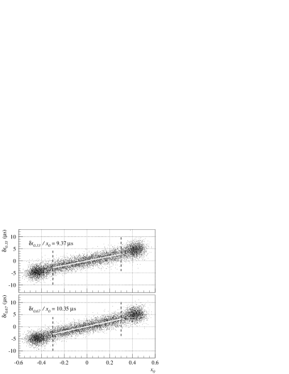
Figure 4: Measured time differences between the two detector channels versus position, for trigger thresholds at 33% (top) and at 67% (bottom) of the signal peak amplitudes. The white lines are linear fits to the data in the range $|x_{0}|<0.3$. The resulting fit parameter is included in the plots.

We have numerically simulated the quasiparticle propagation according to Eq. (2) to determine the detector-signal dynamics including the response of readout electronics and pulse shaping. The normalized timing differences $\delta t_{n}$ between the two channels calculated for trigger thresholds at $33\%$ and $67\%$ were $0.336$ and $0.351$, respectively, assuming $D=L=1$. Scaling the measured data with these results allows us to estimate the diffusion constant

$$D\approx\frac{\delta t_{n}}{2\delta t_{m}\,x_{\mathrm{max}}}L_{\mathrm{Ta}}^{2}\approx 7.8\,\frac{\mathrm{cm}^{2}}{\mathrm{s}}\,.$$

For comparison, a theoretically evaluated diffusion constant is given byNarayanamurti1978

$$D_{\mathrm{th}}=\sqrt{\frac{k_{B}T}{2\pi\Delta}}v_{F}^{2}\tau_{\mathrm{imp}}\,,$$

where $v_{F}=1.6\times 10^{8}\,\mathrm{cm}^{2}\mathrm{s}^{-1}$ is the Fermi velocity of electrons in the superconductor, $\tau_{\mathrm{imp}}=m_{e}/\rho_{{}_{\mathrm{LT}}}ne^{2}$ is the impurity-scattering time, $m_{e}$ is the electron rest mass and $n=5.52\times 10^{22}\,\mathrm{cm}^{-3}$ the density of conduction electrons in Ta.Nussbaumer2000 With $\rho_{{}_{\mathrm{LT}}}=0.5\times 10^{-8}\,\Omega\mathrm{m}$ (or $\rho_{{}_{\mathrm{RT}}}=13\times 10^{-8}\,\Omega\mathrm{m}$ and $RRR=25$, respectively) and at $T=310\,\mathrm{mK}$ we obtain $D_{\mathrm{th}}=25.2\,\mathrm{cm}^{2}\mathrm{s}^{-1}$, which is more than three times the experimentally determined value. Similar discrepancies between experiment and theoretical predictions were systematically observed in other experimentsFriedrich1997 ; Kirk2000 ; Hartog2000 ; Nussbaumer2000 ; Li2003 ; Segall2004 and remain unresolved.

The quasiparticle loss time deduced from the measurements is found to be $\tau_{\mathrm{loss}}=\Lambda^{2}D^{-1}\approx 58.9\,\mu\mathrm{s}$, which is significantly longer than the tunneling time of about $1\,\mu\mathrm{s}$. However, the trapping process with a time constant $\tau_{\mathrm{trap}}=\beta^{2}\tau_{\mathrm{loss}}\approx 18.9\,\mu\mathrm{s}$ should preferably be improved in our devices towards faster trapping rates, in order to enhance $x_{\mathrm{max}}\rightarrow 1$ for better position resolution.

Alternatively to our phenomenological discussion on imaging resolution in the previous section, the resolving capabilities have been derived analyticallyEsposito1994 with a prediction for

$$\delta x\approx\sqrt{D\tau_{\mathrm{loss}}}\frac{q_{i}}{Q_{\sigma}}=\Lambda\frac{q_{i}}{Q_{\sigma}}\,.$$

Inserting our experimental results (always for single-photon events only) yields position resolutions in the range $\delta x\approx 26.7\ldots 14.8\,\mu\mathrm{m}$, corresponding to $5\ldots 9$ pixels for our detector. This is in fair agreement with our former approximations. However, we wish to emphasize that all these rough estimates ignore the geometrical properties of the real absorber, which needs to be taken into account for a quantitatively precise analysis of position resolution.Ejrnaes2005

IV Conclusions

Detection of single (and simultaneous multiple) photons with good spectral and spacial resolution was performed with STJ based DROIDs. Single-photon resolution down to near IR energies was proven, with a perfectly linear energy response over the entire UV to IR wavelength range. Sensitivity to the investigated photon energies was possible due to the backtunneling effect, delivering in our case a device-intrinsic gain of about 33, which is a feature unique to STJs. The detectors were found to operate close to the thermodynamic limit imposed by particle fluctuation statistics.

The measured dynamic response of the DROIDs was compared to numerical modelling based on quasiparticle diffusion including loss and trapping processes. The parameters extracted from experimental data are physically meaningful and coincide reasonably with former Monte Carlo simulations.Jerjen2006 However, the diffusion constant was found to significantly disagree with theoretical predictions, similar to all preceding experiments of the same kind.

Position resolution of our relatively short absorber was estimated to about $3\ldots 6$ equivalent pixels for photon energies in the range $0.8\ldots 3.4\,\mathrm{eV}$. By taking the differential time delays of the two channels into account, we predict an improvement in position resolution by at least a factor of two for a longer absorber ($L_{\mathrm{Ta}}\rightarrow\Lambda$) and better trapping efficiencies ($\tau_{trap}\ll\tau_{loss}$).

High-sensitivity spectrometers with single-photon counting capabilities in the broad optical range are not only of high interest for astronomical observations. Single photons at the telecommunication wavelength of $1550\,\mathrm{nm}$ are currently used, e.g., in intense studies on quantum cryptography,Gisin2002 which links information theory to quantum entanglement physics. Hence, STJ based DROIDs with the properties and potential as presented in this paper may as well be an interesting and natural choice for IR single-photon counting experiments.

- (1) N. E. Booth and D. J. Goldie, Supercond. Sci. Technol. 9, 493 (1996).
- (2) K. E. Gray, Appl. Phys. Lett. 32, 392 (1978).
- (3) M. A. C. Perryman, M. Cropper, G. Ramsay, F. Favata, A. Peacock, N. Rando, and A. Reynolds, Mon. Not. R. Astron. Soc. 324, 899 (2001).
- (4) D. D. E. Martin, P. Verhoeve, A. Peacock, A. van Dordrecht, J. Verveer, and R. Hijmering, Nucl. Instrum. Methods Phys. Res. A 520, 512 (2004).
- (5) H. Kraus, F. von Feilitzsch, J. Jochum, R. L. Mössbauer, Th. Peterreins, and F. Pröbst, Phys. Lett. B 231, 195 (1989).
- (6) J. Jochum, H. Kraus, M. Gutsche, B. Kemmather, F. v. Feilitzsch, and R. L. Mössbauer, Ann. Physik 2, 611 (1993).
- (7) S. Friedrich, K. Segall, M. C. Gaidis, C. M. Wilson, D. E. Prober, A. E. Szymkowiak, and S. H. Moseley, Appl. Phys. Lett. 71, 3901 (1997).
- (8) E. C. Kirk, Ph. Lerch, J. Olsen, A. Zehnder, and H. R. Ott, Nucl. Instrum. Methods Phys. Res. A 444, 201 (2000).
- (9) L. Li, L. Frunzio, K. Segall, C. M. Wilson, D. E. Prober, A. E. Szymkowiak, and S. H. Moseley, Nucl. Instrum. Methods Phys. Res. A 444, 228 (2000).
- (10) R. den Hartog, D. Martin, A. Kozorezov, P. Verhoeve, N. Rando, A. Peacock, G. Brammertz, M. Krumrey, D. J. Goldie, and R. Venn, Proc. SPIE 4012, 237 (2000).
- (11) L. Li, L. Frunzio, C. M. Wilson, and D. E. Prober, J. Appl. Phys. 93, 1137 (2003).
- (12) C. M. Wilson, K. Segall, L. Frunzio, L. Li, D. E. Prober, D. Schiminovich, B. Mazin, C. Martin, and R. Vasquez, Nucl. Instrum. Methods Phys. Res. A 444, 449 (2000).
- (13) P. Verhoeve, R. den Hartog, D. Martin, N. Rando, A. Peacock, and D. J. Goldie, Proc. SPIE 4008, 683 (2000).
- (14) I. Jerjen, E. Kirk, E. Schmid, and A. Zehnder, Nucl. Instrum. Methods Phys. Res. A 559, 497 (2006).
- (15) R. A. Hijmering, P. Verhoeve, D. D. E. Martin, A. Peacock, and A. G. Kozorezov, Nucl. Instrum. Methods Phys. Res. A 559, 689 (2006).
- (16) R. A. Hijmering, P. Verhoeve, D. D. E. Martin, A. Peacock, A. G. Kozorezov, and R. Venn, Nucl. Instrum. Methods Phys. Res. A 559, 692 (2006).
- (17) J. H. Weaver, D. W. Lynch, and C. G. Olson, Phys. Rev. B10, 501 (1974).
- (18) F. Gervais, in Handbook of optical constants of solids II, edited by E. D. Palik (Academic, San Diego, CA, 1991), p. 761.
- (19) M. Kurakado, Nucl. Instrum. Meth. 196, 275 (1982).
- (20) N. Rando, A. Peacock, A. van Dordrecht, C. Foden, R. Engelhardt, B. G. Taylor, P. Gare, J. Lumley, and C. Pereira, Nucl. Instrum. Methods Phys. Res. A 313, 173 (1992).
- (21) A. Zehnder, Phys. Rev. B52, 12858 (1995).
- (22) D. J. Goldie, P. L. Brink, C. Patel, N. E. Booth, and G. L. Salmon, Appl. Phys. Lett. 64, 3169 (1994).
- (23) B. Ivlev, G. Pepe, and U. Scotti di Uccio, Nucl. Instrum. Methods Phys. Res. A 300, 127 (1991).
- (24) E. Esposito, B. Ivlev, G. Pepe, and U. Scotti di Uccio, J. Appl. Phys. 76, 1291 (1994).
- (25) K. Segall, C. Wilson, L. Frunzio, L. Li, S. Friedrich, M. C. Gaidis, D. E. Prober, A. E. Szymkowiak, and S. H. Moseley, Appl. Phys. Lett. 76, 3998 (2000).
- (26) D. D. E. Martin, P. Verhoeve, A. Peacock, A. G. Kozorezov, J. K. Wigmore, H. Rogalla, and R. Venn, Appl. Phys. Lett. 88, 123510 (2006).
- (27) A. G. Kozorezov, A. F. Volkov, J. K. Wigmore, A. Peacock, A. Poelaert, and R. den Hartog, Phys. Rev. B61, 11807 (2000).
- (28) A. Zehnder, Ph. Lerch, S. P. Zhao, Th. Nussbaumer, E. C. Kirk, and H. R. Ott, Phys. Rev. B59, 8875 (1999).
- (29) V. Narayanamurti, R. C. Dynes, P. Hu, H. Smith, and W. F. Brinkman, Phys. Rev. B18, 6041 (1978).
- (30) Th. Nussbaumer, Ph. Lerch, E. Kirk, A. Zehnder, R. Füchslin, P. F. Meier, and H. R. Ott, Phys. Rev. B61, 9719 (2000).
- (31) K. Segall, C. Wilson, L. Li, L. Frunzio, S. Friedrich, M. C. Gaidis, and D. E. Prober, Phys. Rev. B70, 214520 (2004).
- (32) M. Ejrnaes, C. Nappi, and R. Cristiano, Supercond. Sci. Technol. 18, 953 (2005).
- (33) N. Gisin, G. Ribordy, W. Tittel, and H. Zbinden, Rev. Mod. Phys. 74, 145 (2002).