Dynamics of propagating turbulent pipe flow structures. Part I: Effect of drag reduction by spanwise wall oscillation

Abstract

The results of a comparative analysis based upon a Karhunen-Loève expansion of turbulent pipe flow and drag reduced turbulent pipe flow by spanwise wall oscillation are presented. The turbulent flow is generated by a direct numerical simulation at a Reynolds number $Re_{\tau}=150$. The spanwise wall oscillation is imposed as a velocity boundary condition with an amplitude of $A^{+}=20$ and a period of $T^{+}=50$. The wall oscillation results in a 27% mean velocity increase when the flow is driven by a constant pressure gradient. The peaks of the Reynolds stress and root-mean-squared velocities shift away from the wall and the Karhunen-Loève dimension of the turbulent attractor is reduced from $2453$ to $102$. The coherent vorticity structures are pushed away from the wall into higher speed flow, causing an increase of their advection speed of 34% as determined by a normal speed locus. This increase in advection speed gives the propagating waves less time to interact with the roll modes. This leads to less energy transfer and a shorter lifespan of the propagating structures, and thus less Reynolds stress production which results in drag reduction.

I INTRODUCTION

In the last decade a significant amount of work has been performed investigating the structure of wall bounded turbulence, with aims of understanding its self-sustaining nature and discovering methods of control. panton_overview One of the greatest potential benefits for controlling turbulence is drag reduction. As the mechanics of the different types of drag reduction are studied, most explanations of the mechanism revolve around controlling the streamwise vortices and low speed streaks. karniadakis_choi ; choi_nature06 One such method of achieving drag reduction is spanwise wall oscillation, first discovered by Jung et al. jung in 1992, and later confirmed both numerically quadrio ; choi ; jung ; zhou_dongmei ; quadrio2 and experimentally, choiGraham ; trujillo ; choiEXP ; skandaji ; laadhari to reduce drag on the order of 45%. The prevalent theory of the mechanism behind this was developed using direct numerical simulation of a turbulent channel flow by Choi et al. choi and experimentally confirmed by Choi and Clayton, choi_clayton showing that the spatial correlation between the streamwise vortices and the low speed streaks are modified so that high speed fluid is ejected from the wall, and low speed fluid is swept towards the wall. Even though this proposed mechanism describes the near-wall dynamics that govern the drag reduction, questions behind the global dynamics have not been sufficiently resolved. What is the effect (if any) on the outer region of the flow? How do the coherent structures of the flow near the wall adjust with the spanwise oscillations? What is the effect on the interactions between the inner and outer layers?

One manner in which to address these questions is through direct numerical simulation (DNS) of turbulence. As supercomputing resources increase, DNS continues to provide an information rich testbed to investigate the dynamics and mechanisms behind turbulence and turbulent drag reduction. DNS resolves all the scales of turbulence without the need of a turbulent model and provides a three dimensional time history of the entire flow field. One of the methods used for mining the information generated by DNS is the Karhunen-Loève (KL) decomposition, which extracts coherent structures from the eigenfunctions of the two-point spatial correlation tensor. This allows a non-conditionally based investigation that takes advantage of the richness of DNS. The utility of this method is evident in the knowledge it has produced so far, such as the discovery of propagating structures (traveling waves) of constant phase velocity that trigger bursting and sweeping events. sirovich1 ; sirovich2 ; ball These studies in turn have lead to a new class of methods for achieving drag reduction through wall imposed traveling waves. itoh ; karniadakis_choi Another study using KL decomposition examined the energy transfer path from the applied pressure gradient to the flow through triad interaction of structures, webber1 ; webber2 explaining the dynamical interaction between the KL modes. In the realm of control, KL methods have been used to produce drag reduction in a turbulent channel by phase randomization of the structures handler and to understand the effect of drag reduction by controlled wall normal suction and blowing.prabhu In the present study, the KL framework is used to examine the differences in the turbulent structures and dynamics between turbulent pipe flow with and without spanwise wall oscillation.

For this comparative analysis, turbulent pipe flow was chosen as opposed to turbulent channel flow because of its industrial relevance and experimental accessibility. The main difference between pipe and channel flows is that in turbulent pipe flow the mean flow profile exhibits a logarithmic profile that overshoots the theoretical profile at low Reynolds numbers, whereas in turbulent channel flow it does not. patel_head ; durst Secondly, pipe flow differs from channel flow because pipe flow is linearly stable to infinitesimal disturbances where channel flow is linearly unstable above a critical Reynolds number. orszag_patera ; oSullivan_breuer A significant computational difference between pipe and channel flow is the presence of a numerical difficulty introduced by the singularity in polar-cylindrical coordinates at the pipe centerline, which has limited the number of DNS studies in turbulent pipe flow. eggels ; verzicco ; fukagata ; ma ; loulou ; fatica1997 Similarly, many KL studies have been performed in a turbulent channel flow, but to the best of our knowledge the work presented here is the first to extend the KL method to spanwise wall oscillated turbulent pipe flow.

In previous work a DNS of turbulent pipe flow for $Re_{\tau}=150$ was benchmarked and its KL expansion was reported, forming the baseline for this study.duggleby_JOT Similar structures to those of turbulent channel flow sirovich1 ; sirovich2 ; ball were found, including the presence of propagating modes. These propagating modes are characterized by a nearly constant phase speed and are responsible for the Reynolds stress production as they interact and draw energy from the roll modes (streamwise vortices). sirovich1 Without this interaction and subsequent energy transfer, the propagating waves decay quickly, reducing the total Reynolds stress of the flow.kerswell As shown by Sirovich et al., sirovich1 ; sirovich2 the interaction between the propagating waves and the roll modes occurs by the propagating waves forming a coherent oblique plane wave packet. This wave packet interacts with the roll modes, and when given enough interaction time, the roll mode is destabilized eventually resulting in a bursting event. sirovich1 It is in this bursting event that the energy is transferred from the rolls to the propagating waves.webber1 In this paper we show that in the presence of spanwise wall oscillation these propagating modes are pushed away from the wall into higher speed flow. This causes the propagating modes to advect faster, giving them less time to interact with the roll modes. This leads to reduced energy transfer that occurs less often, and yields lower Reynolds stress production, which ultimately results in drag reduction.

II NUMERICAL METHODS

We use a globally high order spectral element Navier-Stokes algorithm to generate turbulent data for pipe flow driven by a mean streamwise pressure gradient. fischer_patera ; tufo The non-dimensional equations governing the fluid are

$$\partial_{t}\mathbf{U}+\mathbf{U}\cdot\nabla\mathbf{U}=-\nabla P+\mathrm{Re}_{\tau}^{-1}\nabla^{2}\mathbf{U}$$ (1)

$$\nabla\cdot\mathbf{U}=0,$$ (2)

where $\mathbf{U}$ is the velocity vector, $\mathrm{Re}_{\tau}$ is the Reynolds number, and $P$ is the pressure. The velocity is non-dimensionalized by the wall shear velocity $U_{\tau}=\sqrt{\tau_{w}/\rho}$ where $\tau_{w}$ is the wall shear stress and $\rho$ is the density. The Reynolds number is $\mathrm{Re}_{\tau}=U_{\tau}R/\nu=150$, where $R$ is the radius of the pipe, and $\nu$ is the kinematic viscosity. When non-dimensionalized with the centerline velocity, the Reynolds number is $Re_{c}\approx 4300$. Two simulations were performed, one with and one without spanwise wall oscillation. In a pipe, the spanwise direction corresponds to the azimuthal direction, so the oscillation is about the axis of the pipe. Each case was run for $t^{+}=U_{\tau}^{2}t/\nu=16800$ viscous time units. In the oscillated case, the simulation was performed with an azimuthal velocity wall boundary condition $v_{\theta}(r=R,\theta,z)=A^{+}\sin(2\pi t/T^{+})$ of amplitude $A^{+}=A/U_{\tau}=20$ and period $T^{+}=U_{\tau}^{2}T/\nu=50$ with $(r,\theta,z)$ being the radial, azimuthal, and streamwise coordinates respectively. This is not intended to be a parametric study and the amplitude and period were chosen to achieve maximum possible drag reduction before relaminarization occurred.

To solve equations 1 and 2 we use a numerical algorithm employing a geometrically flexible yet exponentially convergent spectral element discretization in space. The spatial domain is subdivided into elements, each containing a high-order (12th order) Legendre Lagrangian interpolant. lottes The spectral element algorithm elegantly avoids the numerical singularity found in polar-cylindrical coordinates at the origin, as seen in Figure 1. The streamwise direction contains 40 spectral elements over a length of 10 diameters. The effective resolution of the flow near the wall is $\Delta r^{+}\approx 0.78$ and $(R\Delta\theta)^{+}\approx 4.9$, where the radius $r^{+}$ and the arc length at the wall $(R\Delta\theta)^{+}$ are normalized by wall units $\nu/U_{\tau}$ denoted by the superscript $+$. Near the center of the pipe, the grid width is $\Delta^{+}\approx 3.1$. The grid spacing in the streamwise direction is a constant $\Delta z^{+}=6.25$ throughout the domain. Further details can be found in Duggleby et al.duggleby_JOT

The flow is driven by a constant mean pressure gradient to keep $\mathrm{Re}_{\tau}$ constant. The spanwise wall oscillation results in a mean flow rate increase, effectively changing the Reynolds number based upon mean velocity ($\mathrm{Re}_{m}$) while keeping $\mathrm{Re}_{\tau}$ constant. This keeps the dominant structures of the flow similar, as they are affected primarily by the inner layer wall shear stress.zhou_dongmei The oscillations were started on a fully turbulent pipe at $\mathrm{Re}_{\tau}=150$, and to avoid transient effects, data were not taken until the mean flow rate had settled at its new average value over a time interval of $1000t^{+}$.

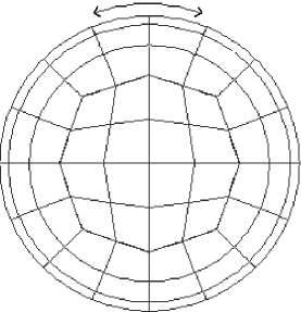
Figure 1: A cross-section of a spectral element grid used for the pipe flow simulation. The arrow denotes the direction of the spanwise (azimuthal) oscillation about the axis of the pipe.

In the Karhunen-Loève (KL) procedure, the eigenfunctions of the two-point velocity correlation tensor, defined by

$$\int_{0}^{L}\int_{0}^{2\pi}\int_{0}^{R}K(\mathbf{x},\mathbf{x}^{\prime})\mathbf{\Phi}(\mathbf{x}^{\prime})r^{\prime}dr^{\prime}d\theta^{\prime}dz^{\prime}=\lambda\mathbf{\Phi}(\mathbf{x}),$$ (3)

$$K(\mathbf{x},\mathbf{x^{\prime}})=\langle\mathbf{u}(\mathbf{x})\otimes\mathbf{u}(\mathbf{x}^{\prime})\rangle,$$ (4)

are obtained, where $\mathbf{x}=(r,\theta,z)$ is the position vector, $\mathbf{\Phi}(\mathbf{x})$ is the eigenfunction with associated eigenvalue $\lambda$, $K(\mathbf{x},\mathbf{x}^{\prime})$ is the kernel, and $\otimes$ denotes an outer product. In order to focus on the turbulent structures, the kernel is built using fluctuating velocities $\mathbf{u}=\mathbf{U}-\overline{\mathbf{U}}$. The mean velocity, $\overline{\mathbf{U}}$, is found by averaging over all $\theta$, $z$, and time. The angle brackets in equation 4 represent the time average using an evenly spaced time interval over a total time period sufficient to sample the turbulent attractor. In this study, the flow field was sampled every $8t^{+}$ for a total time of $16800t^{+}$.

Since the azimuthal and streamwise directions are periodic, the kernel in the azimuthal and streamwise direction is only a function of the distance between $\mathbf{x}$ and $\mathbf{x}^{\prime}$ in those respective directions. Therefore the kernel can be rewritten as

$$K(r,\theta,z,r^{\prime},\theta^{\prime},z^{\prime}) = K(r,r^{\prime},\theta-\theta^{\prime},z-z^{\prime})$$ (5)

$$= \mathcal{K}(m,n;r,r^{\prime})e^{in\theta}e^{i2\pi mz/L}$$

with azimuthal and streamwise wavenumbers $n$ and $m$ respectively and the remaining two-point correlation in the radial direction $\mathcal{K}(m,n;r,r^{\prime})$. It can be shown that in this form, the Fourier series is the resulting KL function in the streamwise and azimuthal direction. Holmes The resulting eigenfunction then takes the form

$$\mathbf{\Phi}(r,\theta,z)=\mathbf{\Psi}(m,n;r)e^{in\theta}e^{i2\pi mz/L}.$$ (6)

Making use of this result, and noting that the two-point correlation in a periodic direction is simply the Fourier transform of the velocities, the azimuthal and streamwise contributions to the eigenfunctions are extracted a priori by taking the Fourier transform of the velocities $\mathbf{u}(r,\theta,z)=\sum_{m,n=0}^{\infty}\hat{\mathbf{u}}(m,n;r)e^{in\theta}e^{i2\pi mz/L}$ and forming the remaining kernel $\mathcal{K}(m,n;r,r^{\prime})$ for each wavenumber pair $n$ and $m$. The eigenfunction problem, with the orthogonality of the Fourier series taken into account, is

$$\int_{0}^{R}\mathcal{K}(m,n;r,r^{\prime})\mathbf{\Psi}^{\star}(r^{\prime})r^{\prime}dr^{\prime}=\lambda_{mn}\mathbf{\Psi}(m,n;r),$$ (7)

$$\mathcal{K}(m,n;r,r^{\prime})=\langle\hat{\mathbf{u}}(m,n;r)\otimes\hat{\mathbf{u}}^{\star}(m,n;r^{\prime})\rangle.$$ (8)

where the $\star$ denotes the complex conjugate since the function is now complex, and the weighting function $r^{\prime}$ is present because the inner product is evaluated in polar-cylindrical coordinates. The final form is still Hermitian just as it was in equation 3; the discrete form of equation 7 is kept Hermitian by splitting the integrating weight and solving the related eigenvalue problem

$$\left[\sqrt{r_{p}}\mathbf{\mathcal{K}}_{ps}(m,n;r_{p},r_{s})\sqrt{r_{s}}\right]\left[\sqrt{r_{s}}\mathbf{\Psi}_{q}(m,n;r_{s})\right]^{\star}$$

$$=\lambda_{mnq}\left[\sqrt{r_{p}}\mathbf{\Psi}_{q}(m,n,;r_{p})\right],$$ (9)

where $\mathbf{\mathcal{K}}_{ps}(m,n;r_{p},r_{s})$ is the discretization of $\mathcal{K}(m,n;r,r^{\prime})$ using a $Q$ point quadrature to evaluate equation 7 with $p,s=1,2,...,Q$. Because the kernel is built with the two-point correlation between all three coordinate velocities, its solution has $3Q$ complex eigenfunctions $\mathbf{\Psi}_{q}$ and corresponding eigenvalues, listed in decreasing order $\lambda_{mnq}>\lambda_{mn(q+1)}$ for a given $m$ and $n$, with quantum number $q=1,2,...,3Q$. It is noted that equation II is only valid for a trapezoidal integration scheme with evenly spaced grid points (which was used in this study), a different quadrature with weight $w(r)$ can be incorporated in a similar fashion, keeping the final matrix Hermitian.

The eigenfunctions$\mathbf{\Psi}_{q}(m,n;r)$ hold certain properties. Firstly, they are normalized with inner product of unit length $\int_{0}^{R}\mathbf{\Psi}_{q},\mathbf{\Psi}_{q^{\prime}}rdr=\delta_{qq^{\prime}}$, where $\delta$ is the Kronecker delta. Secondly, since the eigenfunctions represent a flow field,

$$\mathbf{\Psi}_{q}(m,n;r)=\left(\Psi^{r}_{q}(m,n;r),\Psi^{\theta}_{q}(m,n;r),\Psi^{z}_{q}(m,n;r)\right)^{T}$$ (10)

with radial, azimuthal, and streamwise components $\Psi^{r}_{q}(m,n;r)$, $\Psi^{\theta}_{q}(m,n;r)$, and $\Psi^{z}_{q}(m,n;r)$ respectively, they hold the properties of the flowfield such as boundary conditions (no slip) and continuity

$$\frac{1}{r}\frac{d}{dr}(r\Psi^{r}_{q}(m,n;r))+\frac{in}{r}\Psi^{\theta}_{q}(m,n;r)+\frac{i2\pi m}{L}\Psi^{z}_{q}(m,n;r)=0.$$ (11)

Thirdly, the eigenvalues represent the average energy of the flow contained in the eigenfunction $\mathbf{\Psi}_{q}(m,n;r)$

$$\lambda_{mnq}=\langle|\mathbf{u}(r,\theta,z),\mathbf{\Psi}_{q}(m,n;r)e^{in\theta}e^{i2\pi mz/L}|^{2}\rangle,$$ (12)

which is why it is necessary that the discrete matrix in equation II must be Hermitian to get real and positive eigenvalues. These three properties allow the eigenfunctions to be tested for their validity.

In summary, the KL procedure yields an orthogonal set of basis functions (modes) that are the most energetically efficient expansion of the flow field. By studying the subset that includes the largest energy modes, insight is gained as this subset forms a low dimensional model of the given flow. Examining the structure, dynamics, and interactions of this low dimensional model yields important information that we use to build a better understanding of the dynamics of the entire system.

III RESULTS

Spanwise wall oscillation results in four main effects on the flow, its structures, and its dynamics. They are:

1. An increase in flow rate and a shifting away from the wall of the root-mean-squared velocities and Reynolds stress peaks.

2. A reduction in the dimension of the chaotic attractor describing the turbulence.

3. An increase in energy of the propagating modes responsible for carrying energy away from the wall to the upper region, while the rest of the propagating modes exhibit a decrease in energy.

4. An increase of the advection speed of the traveling wave packet as determined by a normal speed locus.

First, surface oscillation has a major effect on the turbulent statistics. The spanwise wall oscillation of amplitude $A^{+}=20$ and period $T^{+}=50$ resulted in a flow rate increase of 26.9%, shown in Figure 2. This combination of amplitude and period was chosen because it provides the largest amount of drag reduction while keeping the flow turbulent. Numerical simulations with larger oscillations completely relaminarize the flow. The comparison of the mean profiles in Figures 3 and 4 show the higher velocity in the outer region, with the inner region remaining the same, as expected by keeping a constant mean pressure gradient across the pipe.

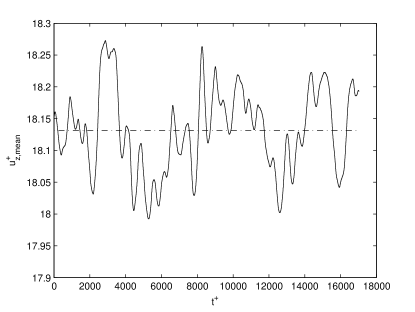
Figure 2: Mean velocity fluctuations (solid) and the average velocity (dash-dot) for the oscillated case versus time ($t^{+}$). The fluctuations are consistent with turbulent flow, and the mean velocity is 26.9% greater than in the non-oscillated pipe.

Figure 3: Mean velocity profile for a non-oscillated (solid) and oscillated (dashed) turbulent pipe flow versus $y^{+}$. Theoretical (dash-dot) includes the sublayer ($u^{+}=y^{+}$) and the log layer ($u^{+}=\log(y^{+})/0.41+5.5$). The mean profile shows a log layer, but overshoots the theoretical value as expected for pipe flow until a much higher Reynolds number.

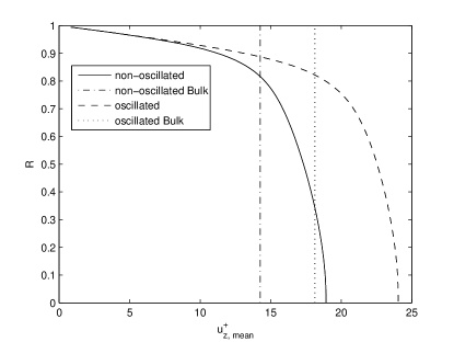
Figure 4: Mean velocity profile for non-oscillated (solid) and oscillated (dashed) pipes with their respective bulk velocities (dash-dot and dots) versus radius show an increase in bulk velocity of 26.9%.

The comparison of the root-mean-square (rms) velocity fluctuation profiles and the Reynolds stress profile in Figures 5 and 6 show that the streamwise fluctuations decrease in intensity by 7.5% from 2.68 to 2.48. Also, the change in peak location from $y^{+}=16$ to $y^{+}=22$ away from the wall has the same trend as the maximum Reynolds stress $\overline{u_{r}u_{z}}$, where $y^{+}=(R-r)U_{\tau}/\nu$ is the distance from the wall using normalized wall units ($\nu/U_{\tau}$). The azimuthal fluctuating velocities show a slightly greater magnitude peak of 1.03 closer to the wall at $y^{+}=29$ versus 0.99 at $y^{+}=40$ for the non-oscillated pipe. The radial fluctuations remain almost unchanged, showing only a slight decrease from the wall through the log layer ($y^{+}\approx 100$), resulting in the peak shifting from 0.81 at $y^{+}=55$ to 0.78 at $y^{+}=61$. The Reynolds stress also shows a reduction in strength and a shift away from the wall. The peak changes from 0.68 at $y^{+}=31$ to 0.63 at $y^{+}=38$. Thus, a major difference between the two flow cases, in addition to the expected flow rate increase, is the shift of the rms velocity and Reynolds stress peaks away from the wall.

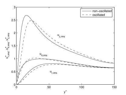
Figure 5: Root-mean-squared velocity fluctuations for the non-oscillated (solid) and oscillated (dashed) case versus $y^{+}$. The oscillated case shows a shift away from the wall, except for the azimuthal rms which captures the Stokes layer imposed by the wall oscillation.

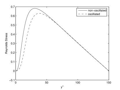
Figure 6: Reynolds Stress $\overline{u_{r}u_{z}}$ versus $y^{+}$ for non-oscillated (solid) and oscillated (dashed) cases. Similar to the rms velocities, the Reynolds stress shows a shift away from the wall from $y^{+}=31$ to $y^{+}=38$.

The second major effect can be found by examining the size of the chaotic attractor describing the turbulence. The eigenvalues of the KL decomposition represent the energy of each eigenfunction. By ordering the eigenvalues from largest to smallest, the number of eigenfunctions needed to capture a given percentage of energy of the flow is minimized. Table 1 shows the 25 most energetic eigenfunctions, and Figure 7 shows the running total of energy versus mode number. 90% of the energy is reached with $D_{KL}=102$ compared to $D_{KL}=2453$ for the non-oscillated case. This mark, known as the Karhunen-Loève dimension, is a measure of the intrinsic dimension of the chaotic attractor of turbulence as discussed by Sirovich sirovich_chaos ; zhou_sirovich . By oscillating the wall our results show that the size of the attractor is reduced, and the system is less chaotic.

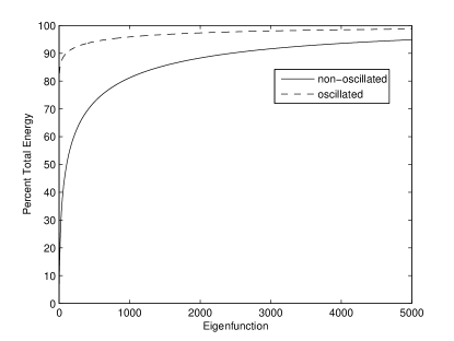
Figure 7: Comparison of the running total energy retained in the KL expansion for the non-oscillated (solid) and oscillated (dashed) cases. The 90% crossover point is 2453 and 102 respectively. This shows a drastic reduction in the dimension of the chaotic attractor.

The third major effect is found by examining the energy of the eigenfunctions. The 25 most energetic are listed for each case in Table 1. The top ten modes with the largest change in energy are shown in Table 2. Firstly, the order of the eigenfunctions remain relatively unchanged, with a few notable differences. The (0,0,1) and (0,0,3) shear modes represent the Stokes flow as seen in Figures 8a and 8c, and the (0,0,2) mode, shown in Figure 8b, represents the changing of the mean flow rate, similar to the non-oscillated (0,0,1) mode. The (1,2,1) mode shows a large increase in energy. Also of note is the reduction in energy of the (3,1,1) and (4,1,1) modes, but their structure remains virtually unchanged.

Table 1: The 25 most energetic modes; $m$ is the streamwise wavenumber, $n$ is the spanwise wavenumber, and $q$ is the eigenvalue quantum number.

	Non-oscillated						Oscillated
Index	$m$	$n$	$q$	Energy	% Total		$m$	$n$	$q$	Energy	% Total
1	0	6	1	1.61	2.42%		0	0	1	216	68.77%
2	0	5	1	1.48	2.22%		0	0	2	34.7	11.07%
3	0	3	1	1.45	2.17%		1	2	1	2.47	0.79%
4	0	4	1	1.29	1.93%		0	3	1	2.30	0.73%
5	0	2	1	1.26	1.88%		0	1	1	2.27	0.73%
6	1	5	1	0.936	1.40%		0	2	1	2.20	0.70%
7	1	6	1	0.917	1.37%		0	4	1	1.49	0.48%
8	1	3	1	0.902	1.35%		1	3	1	1.09	0.35%
9	1	4	1	0.822	1.23%		0	5	1	1.04	0.33%
10	0	1	1	0.805	1.20%		1	1	1	0.953	0.30%
11	1	7	1	0.763	1.14%		1	4	1	0.772	0.25%
12	1	2	1	0.683	1.02%		0	6	1	0.653	0.21%
13	0	7	1	0.646	0.97%		0	0	3	0.616	0.20%
14	2	4	1	0.618	0.92%		1	5	1	0.582	0.19%
15	0	8	1	0.601	0.90%		1	6	1	0.542	0.17%
16	2	5	1	0.580	0.87%		2	3	1	0.490	0.16%
17	1	1	1	0.567	0.85%		0	1	2	0.482	0.15%
18	2	7	1	0.524	0.78%		2	4	1	0.468	0.15%
19	1	8	1	0.483	0.72%		2	5	1	0.444	0.14%
20	2	6	1	0.476	0.71%		0	7	1	0.407	0.13%
21	2	3	1	0.454	0.68%		1	7	1	0.373	0.12%
22	2	2	1	0.421	0.63%		2	6	1	0.346	0.11%
23	2	8	1	0.375	0.56%		2	2	1	0.337	0.11%
24	1	9	1	0.358	0.54%		3	5	1	0.317	0.10%
25	3	4	1	0.354	0.53%		3	3	1	0.290	0.09%

Table 2: Ranking of eigenfunctions by energy change between the non-oscillated and the oscillated cases. $m$ is the streamwise wavenumber, $n$ is the spanwise wavenumber, and $q$ is the eigenvalue quantum number.

	Increase					Decrease
Rank	$\Delta\lambda_{\mathbf{k}}$	$m$	$n$	$q$		$\Delta\lambda_{\mathbf{k}}$	$m$	$n$	$q$
1	215	0	0	1		-0.962	0	6	1
2	34.5	0	0	2		-0.442	0	5	1
3	1.79	1	2	1		-0.390	1	7	1
4	1.47	0	1	1		-0.382	0	8	1
5	0.95	0	2	1		-0.374	1	6	1
6	0.85	1	3	1		-0.353	1	5	1
7	0.49	0	0	3		-0.256	1	8	1
8	0.37	1	1	1		-0.245	2	7	1
9	0.26	0	1	2		-0.239	0	7	1
10	0.20	0	4	1		-0.220	2	8	1

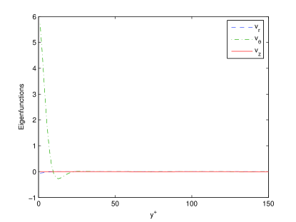
Figure 8a: (0,0,1) eigenfunction capturing the imposed velocity oscillations. The radial velocity is zero except near the wall, where a slight non-zero component is evident, induced by the spanwise oscillation.

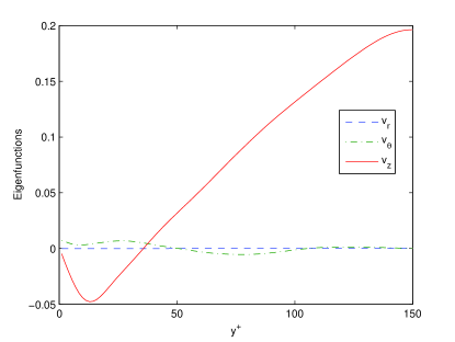
Figure 8b: (0,0,2) eigenfunction, similar in structure to the non-oscillated (0,0,1).

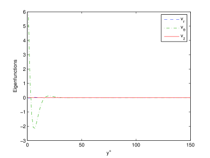
Figure 8c: (0,0,3) eigenfunction capturing the secondary flow in the Stokes layer. This imposed Stokes flow created by the oscillation dominates the near wall region of the oscillated pipe.

In examining the energy content of the structure subclasses as a whole, a trend is discovered, shown in Table 3. Each of these subclasses, reported in Duggleby et al., duggleby_JOT were found to have similar qualitative coherent vorticity structure associated with their streamwise and azimuthal wavenumber. We use “coherent vorticity” to refer to the imaginary part of the eigenvalues of the strain rate tensor $\partial u_{i}/\partial x_{j}$, following the work of Chong et al.. chong Based upon the qualitative structure, the propagating or traveling waves, described by non-zero azimuthal wavenumber and nearly constant phase speed, were found to have four subclasses: the wall, the lift, the asymmetric, and the ring modes.

The wall modes are found when the spanwise wavenumber is larger than the streamwise wavenumber. They possess a qualitative structure having coherent vortex cores near the wall, and have their energy decreased by 20.4% with wall oscillation. Likewise, the ring modes, which are found for non-zero streamwise wavenumber and zero spanwise wavenumber with rings of coherent vorticity, have their energy decreased by 5.2% with wall oscillation. The asymmetric modes have non-zero streamwise wavenumber and spanwise wavenumber $n=1$, which allows them to break azimuthal symmetry. These modes undergo a decrease in energy of 2.3% with spanwise wall oscillation.

Conversely to the decrease in energy found in the other three propagating modes, the lift modes increase in energy by 1.5% with spanwise wall oscillation. These modes are found with a streamwise wavenumber that is greater than the spanwise wavenumber, and they display coherent vortex structures that starts near the wall and lifts away from the the wall to the upper region. Combined, the four propagating subclasses modes lose 9.02% of their energy, whereas the non-propagating modes (the modes with zero azimuthal wavenumber) gain 2043%.

Thus, the third major result is that the energy of the propagating wall, ring, and asymmetric modes decrease while the energy of lift mode increases slightly. Following the work of Sirovich et al. sirovich2 this shows that energy transfer from the streamwise rolls to the traveling waves is reduced, and any energy that is transferred is quickly moved away from the wall to the outer region (lift modes). The energy spectra showing the change of energy by subclasses is shown in Figure 9.

Table 3: Energy comparison of turbulent pipe flow structure subclasses between non-oscillated and oscillated pipes. $m$ is the streamwise wavenumber, and $n$ is the azimuthal (spanwise) wavenumber. All the propagating modes decrease in energy, except the lift modes.

Structure	Energy
	Non-oscillated	Oscillated
Propagating Modes $(m>0)$	53.48	48.86
(a) Wall $(n>m)$	23.5	18.7
(b) Lift $(m\geq n)$	19.8	20.1
(c) Asymmetric $(n=1)$	6.07	5.93
(d) Ring $(n=0)$	4.41	4.18
Non-propagating Modes $(m=0)$	12.97	265
(a) Roll mode $(n>0)$	12.3	13.2
(b) Shear mode $(n=0)$	0.72	251.8

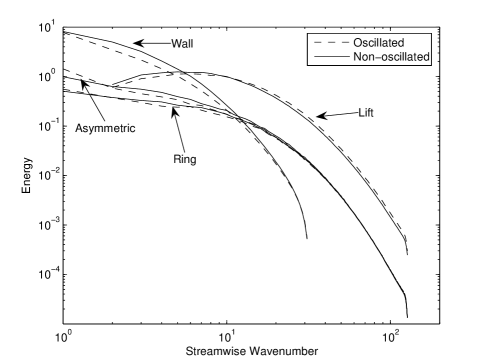
Figure 9: Comparison of energy spectra for non-oscillated (solid) and oscillated (dashed) flows for the propagating mode subclasses. All propagating subclasses in the oscillated case decrease with respect to the non-oscillated case, except for the lift mode, which increases slightly.

The fourth and most important effect is that the propagating modes advect faster in the oscillated case. The normal speed locus of the 50 most energetic modes of both cases is shown in Figure 10. For this, the phase speed $\omega/\|\mathbf{k}\|$ is plotted in the direction $\mathbf{k}/\|\mathbf{k}\|$ with $\mathbf{k}=(m,n)$. A circular locus is evidence that these structures propagate as a wave packet or envelope that travels with a constant advection speed. The advection speed is given by the intersection of the circle with the abscissa. By examining the normal speed locus of the non-oscillated and oscillated pipe flow, the wave packet shows an increase in advection speed from $8.41U_{\tau}$ to $10.96U_{\tau}$, an increase of 30%. This is a result of the oscillating Stokes layer pushing the structures away from the wall into a faster mean flow by creating a dominant near wall Stokes layer where the turbulent structures cannot form. This is confirmed by the shifting of the rms velocities and Reynolds stresses away from the wall as reported earlier. In addition to a faster advection speed, the energy of the propagating modes decay faster, resulting in bursting events with a shorter lifespan. This is seen in Figure 11 where the average burst duration of the (1,5,1) mode is reduced from $106t^{+}$ in the non-oscillated case to $65.3t^{+}$ in the oscillated case. The burst duration is taken to be the average time of all events where the square of the amplitude of the mode is more than one standard deviation greater than the mean.

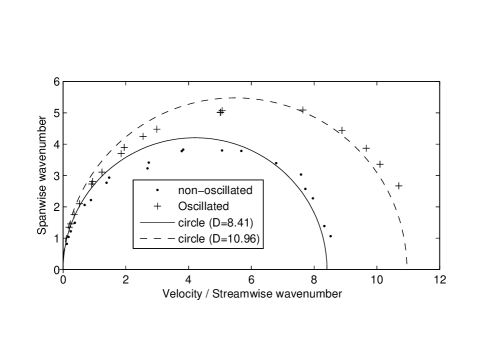
Figure 10: Comparison of the normal speed locus for the oscillated ($\cdot$) and non-oscillated ($+$) case. The solid and dashed lines represent a circle of diameter 8.41 and 10.96 respectively that intersect at the origin.

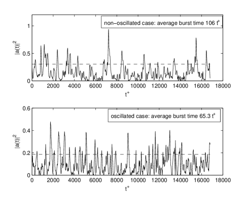
Figure 11: A reduction in the burst duration of the (1,5,1) mode from $106t^{+}$ for the non-oscillated case (top) to $65.3t^{+}$ in the oscillated case (bottom) shows a faster decay of the bursting energy with spanwise wall oscillation. The burst duration is the average time of all events where the square of the amplitude ($|a(t)|^{2}$) is more that one standard deviation greater than the mean. This amplitude level is denoted by the dashed line.

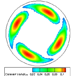
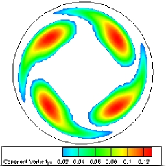
Figure 12: Cross-section of coherent vorticity of (1,2,1) wall mode. Left: (a) non-oscillated. Right: (b) oscillated. The vortex core shifts $y^{+}=6.8$ away from the wall.

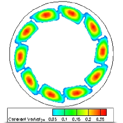
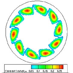
Figure 13: Cross-section of coherent vorticity of (1,5,1) wall mode. Left: (a) non-oscillated. Right: (b) oscillated. The vortex core shifts $y^{+}=9.9$ away from the wall.

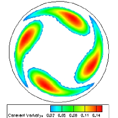
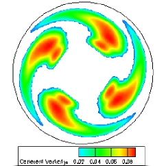
Figure 14: Cross-section of coherent vorticity of (2,2,1) lift mode. Left: (a) non-oscillated. Right: (b) oscillated. The vortex core shifts $y^{+}=11.0$ away from the wall.

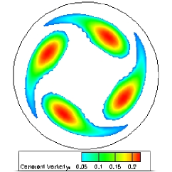
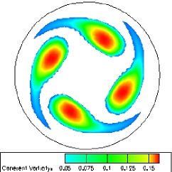
Figure 15: Cross-section of coherent vorticity of (3,2,1) lift mode. Left: (a) non-oscillated. Right: (b) oscillated. The vortex core shifts $y^{+}=11.2$ away from the wall.

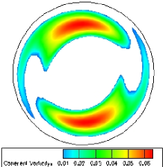
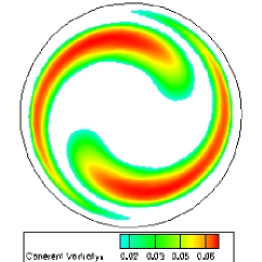
Figure 16: Cross-section of coherent vorticity of (1,1,1) asymmetric mode. Left: (a) non-oscillated. Right: (b) oscillated. The vortex core shifts $y^{+}=3.2$ away from the wall.

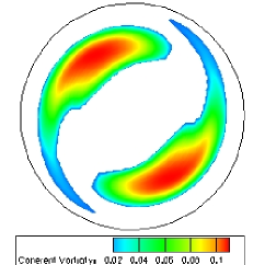
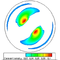
Figure 17: Cross-section of coherent vorticity of (2,1,1) asymmetric mode. Left: (a) non-oscillated. Right: (b) oscillated. The vortex core shifts $y^{+}=45.9$ away from the wall with a slight change in structure.

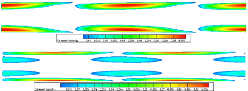
Figure 18: Cross-section along the $r$-$z$ plane of coherent vorticity of (1,0,1) ring mode. Top: (a) non-oscillated. Bottom: (b) oscillated. The vortex core shifts $y^{+}=13$ towards the wall with significant changes in structure.

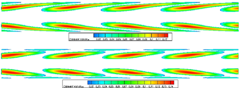
Figure 19: Cross-section along the $r$-$z$ plane of coherent vorticity of (2,0,1) ring mode. Top: (a) non-oscillated. Bottom: (b) oscillated. The vortex core shifts $y^{+}=7$ away from the wall.

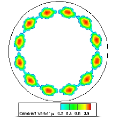
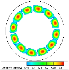
Figure 20: Cross-section of coherent vorticity of (0,6,1) roll mode. Left: (a) non-oscillated. Right: (b) oscillated. The vortex core shifts $y^{+}=10.1$ away from the wall.

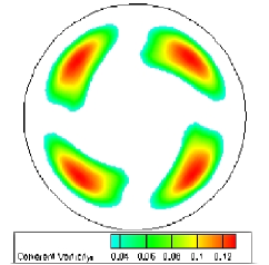
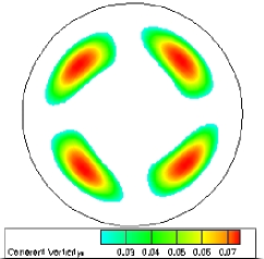
Figure 21: Cross-section of coherent vorticity of (0,2,1) roll mode. Left: (a) non-oscillated. Right: (b) oscillated. The vortex core shifts $y^{+}=7.8$ away from the wall.

The shifting of the structures away from the wall is shown for the most energetic modes for each propagating subclass in Figures 12 through 21. These structures, which represent the coherent vorticity of the four subclasses of the propagating modes, are pushed towards the center of the pipe, where the mean flow velocity is faster. The location of the coherent vortex core for these eight modes are listed in Table 4, showing a shift away from the wall. The only mode found not to follow this trend is the (1,0,1) mode, which undergoes a major restructuring resulting in its vortex core moving towards the wall.

Table 4: Comparison of the measured location of the coherent vortex core for two modes from each propagating subclass in wall units ($y^{+}$) away from the pipe wall . Each class shifts away from the wall, consistent with the shift in velocity rms and Reynolds stress. The (1,0,1) mode changes structure significantly in the oscillated case as seen in Figure 18, explaining the shift of its coherent vortex core towards the wall.

	Coherent vortex core location (wall units)
Mode	Non-oscillated	Oscillated	shift
(1,2,1)	41.8	48.6	6.8
(1,5,1)	28.7	38.6	9.9
(2,2,1)	45.6	56.2	11.0
(3,2,1)	65.9	77.1	11.2
(1,1,1)	47.2	50.4	3.2
(2,1,1)	53.9	99.8	45.9
(1,0,1)	31.9	18.9	-13.0
(2,0,1)	58.4	65.8	7.4
(0,6,1)	28.9	39.0	10.1
(0,2,1)	45.1	52.9	7.8

This faster advection explains the experimental results found by K.-S. Choi choi_kwing that showed a reduction in the duration and strength of sweep events in a spanwise wall oscillated boundary layer of 78% and 64% respectively. For this experiment, the flowrate was kept constant, so the energy was reduced, whereas in our case the mean pressure gradient was kept constant yielding virtually no change in the energy of the propagating structures. Also corroborating these results is the work by Prabhu et al. prabhu that examined the KL decomposition of controlled suction and blowing to reduce drag in a channel. They, too, found that the structures were pushed away from the wall and that they had higher phase velocities. Thirdly, the study by Zhou zhou_dongmei is also consistent with these results, as she found that any oscillation in the streamwise direction reduces the effectiveness of the drag reduction. Any streamwise oscillation, even though it would still push the structures away from the wall, would adversely effect the mean flow rate profile resulting in an advection speed of the propagating waves that is less than in the purely spanwise oscillated case.

Thus, faster advection can be interpreted in two fashions. The first is in terms of the traveling wave. The shifting of the structures away from the wall into higher velocity mean flow causes these structures to travel faster, giving them less interaction time with the roll modes. Less interaction time with the roll modes means less energy transfer (less bursting), and due to their fast decaying nature, their lifetime is reduced. This reduced lifetime means they have less time to generate Reynolds stress, and therefore drag is reduced. The second interpretation is in terms of the classically observed hairpin and horseshoe vortices. theodorsen ; robinson1991 The pushing of the KL structures away from the wall is equivalent to the vortices lifting and stretching away from the wall faster. This faster lifting and stretching process means that their lifetime is shortened, again resulting is less time to generate Reynolds stress, and therefore drag reduction occurs.

IV CONCLUSIONS

This work has shown, through a Karhunen-Loève analysis, four major consequences of spanwise wall oscillation on the turbulent pipe flow structures. They are: a shifting of rms velocities and Reynolds stress away from the wall; a reduction in the dimension of the chaotic attractor describing the turbulence; a decrease in the energy in the propagating modes as a whole with an increase in modes that transfer energy to the outside of the log layer; and a shifting of the propagating structures away from the wall into higher speed flow resulting in faster advection and shorter lifespans, providing less time to generate Reynolds stress and therefore reducing drag.

The strength of the KL method is that it yields global detail and structure without conditional sampling. The ensemble was created out of evenly spaced flowfields in time, as opposed to conditional sampling of the flowfield with event detection such as bursts or sweeps, and the entire flowfield and time history was studied. Therefore, we argue that the overall mechanism of drag reduction through spanwise wall oscillation has been found. Although a result of drag reduction is the decorrelation of the low speed streaks and the streamwise vortices, as found by previous researchers, this is an incomplete description of the dynamics. It is the lifting of the turbulent structures away from the wall by the Stokes flow induced by the spanwise wall oscillation that cause the reduction in the time and duration of Reynolds stress generating events, resulting in drag reduction. In addition, this dynamical description encompasses other methods of drag reduction such as suction and blowing, active control, and ribblets, prabhu establishing it as a contender for a universal theory of drag reduction.

References

- (1) R. Panton, “Overview of the self-sustaining mechanisms of wall turbulence”, Prog. Aero. Sci. 37, 343–383 (2001).
- (2) G. E. Karniadakis and K. S. Choi, “Mechanisms on transverse motions in turbulent wall flows”, Ann. Rev. Fluid Mech. 35, 45–62 (2003).
- (3) K. S. Choi, “Fluid dynamics - the rough with the smooth”, Nature 440, 7085 (2006).
- (4) W. Jung, N. Mangiavacchi, and R. Akhavan, “Suppression of turbulence in wall-bounded flows by high-frequency spanwise oscillations”, Phys. Fluids A 4, 1605 (1992).
- (5) M. Quadrio and S. Sibilla, “Numerical simulation of turbulent flow in a pipe oscillating around its axis”, J. Fluid. Mech. 424, 217 (1999).
- (6) J. Choi, C. Xu, and S. Hyung, “Drag reduction by spanwise wall oscillation in wall-bounded turbulent flows”, AIAA J 40, 842 (2002).
- (7) D. Zhou, “Drag reduction by a wall oscillation in a turbulent channel flow”, University of Texas at Austin, Ph. D. Dissertation (2005).
- (8) M. Quadrio and P. Ricco, “Critical assessment of turbulent drag reduction through spanwise wall oscillations”, J. Fluid. Mech 521, 251 (2004).
- (9) K. S. Choi and M. Graham, “Drag reduction of turbulent pipe flow by circular-wall oscillation”, Phys. Fluids 10, 7 (1998).
- (10) S. M. Trujillo, D. G. Bogard, and K. S. Ball, “Turbulent boundary layer drag reduction using an oscillating wall”, AIAA Paper 97, 1870 (1997).
- (11) K. S. Choi, J. R. BeBisschop, and B. Clayton, “Turbulent boundary-layer control by means of spanwise-wall oscillation”, AIAA Paper 97, 1795 (1997).
- (12) L. Skandaji, “Etude de la structure d’une couche limite turbulente soumis a des oscillations transversales de la paroi”, Ecole Centrale de Lyon, France, Ph.D. Di andssertation (1997).
- (13) L. S. F. Laadhari and R. Morel, “Turbulence reduction in a boundary layer by a local spanwise oscillating surface”, Phys. Fluids A 6, 3218 (1994).
- (14) K. S. Choi and B. R. Clayton, “The mechanism of turbulent drag reduction with wall oscillation”, Int. J. Heat Fluid Flow 22, 1–9 (2002).
- (15) L. Sirovich, K. S. Ball, and L. R. Keefe, “Plane waves and structures in turbulent channel flow.”, Phys. Fluids A 12, 2217–2226 (1990).
- (16) L. Sirovich, K. S. Ball, and R. A. Handler, “Propagating structures in wall-bounded turbulent flows”, Theoret. Comput. Fluid Dynamics 2, 307 (1991).
- (17) K. S. Ball, L. Sirovich, and L. R. Keefe, “Dynamical eigenfunction decomposition of turbulent channel flow”, Int. J. Num. Meth. Fluids 12, 587 (1991).
- (18) M. Itoh, S. Tamano, K. Yokota, and S. Taniguchi, “Drag reduction in a turbulent boundary layer on a flexible sheet undergoing a spanwise traveling wave motion”, J. Turb. 7, 1–17 (2006).
- (19) G. A. Webber, R. A. Handler, and L. Sirovich, “The Karhunen-Loève decomposition of minimal channel flow”, Phys. Fluids 9, 1054–1066 (1997).
- (20) G. A. Webber, R. A. Handler, and L. Sirovich, “Energy dynamics in a turbulent channel flow using the Karhunen-Loève approach”, Int. J. Numer. Meth. Fluids 40, 1381–1400 (2002).
- (21) R. A. Handler, E. Levich, and L. Sirovich, “Drag reduction in turbulent channel flow by phase randomization”, Physics of Fluids A 5, 686–694 (1993).
- (22) R. D. Prabhu, S. S. Collis, and Y. Chang, “The influence of control on proper orthogonal decomposition of wall-bounded turbulent flows”, Phys. Fluids 13, 520–537 (2001).
- (23) V. C. Patel and M. S. Head, “Some observations on skin friction and velocity profiles in fully developed pipe and channel flows”, J. Fluid Mech. 38, 181 (1969).
- (24) F. Durst, J. Jovanovic, and J. Sender, “LDA measurements in the near-wall region of a turbulent pipe flow”, J. Fluid Mech. 295, 305 (1995).
- (25) S. A. Orszag and A. T. Patera, “Secondary instabiliy in wall-bounded shear flows”, J. Fluid Mech. 128, 347 (1983).
- (26) P. L. O’Sullivan and K. S. Breuer, “Transient growth in circular pipe flow. 1. linear disturbances”, Phys. Fluids 6, 3643 (1994).
- (27) J. G. M. Eggels, F. Unger, M. H. Weiss, J. Westerweel, R. J. Friedrich, and F. T. M. Nieuwstadt, “Fully developed turbulent pipe flow: a comparison between direct numerical simulation and experiment”, J. Fluid Mech. 268, 175 (1994).
- (28) R. Verzicco and P. Orlandi, “A finite-difference scheme for three-dimensional incompressible flows in cylindrical coordinates”, J. Comp. Phys 123, 402 (1996).
- (29) K. Fukagata and N. Kasagi, “Highly energy-conservative finite difference method for the cylindrical coordinate system”, J. Comp. Phys. 181, 478 (2000).
- (30) H. Shan, B. Ma, Z.Zhang, and F. T. M. Nieuwstadt, “Direct numerical simulation of a puff and a slug in transitional cylindrcal pipe flow”, J. Fluid Mech. 387, 39 (1999).
- (31) P. Loulou, R. D. Moser, N. N. Mansour, and B. J. Cantwell, “Direct numerical simulation of incompressible pipe flow using a B-spline spectral method”, NASA Technical Memorandum 110436 (1997).
- (32) P. Orlandi and M. Fatica, “Direct numerical simulations of turbulent flow in a pipe rotating about its axis”, J. Fluid Mech. 343, 43–72 (1997).
- (33) A. Duggleby, K. S. Ball, M. R. Paul, and P. F. Fischer, “Dynamical eigenfunction decomposition of turbulent pipe flow”, J. of Turbulence (2006), submitted. ArXiv:physics/0608257, http://lanl.arxiv.org/pdf/physics/0608257.
- (34) R. R. Kerswell, “Recent progress in understanding the transition to turbulence in a pipe”, Nonlinearity 18, R17–R44 (2005).
- (35) P. F. Fischer, L. W. Ho, G. E. Karniadakis, E. M. Ronouist, and A. T. Patera, “Recent advances in parallel spectral element simulation of unsteady incompressible flows”, Comput. & Struct. 30, 217–231 (1988).
- (36) H. M. Tufo and P. F. Fischer, “Terascale spectral element algorithms and implementations”, in Proc. of the ACM/IEEE SC99 Conf. on High Performance Networking and Computing (IEEE Computer Soc.) (1999), gordon Bell Prize paper.
- (37) J. W. Lottes and P. F. Fischer, “Hybrid multigrid/Schwarz algorithms for the spectral element method”, J. Sci. Comp. 24, 45–78 (2004).
- (38) P. Holmes, J. L. Lumley, and G. Berkooz, Turbulence, coherent structures, dynamical systems, and symmetry (Cambridge University Press, Cambridge, UK) (1996).
- (39) L. Sirovich, “Chaotic dynamics of coherent structures”, Phys. D 37, 126 (1989).
- (40) X. Zhou and L. Sirovich, “Coherence and chaos in a model of the turbulent boundary layer”, Phys. Fluids A 4, 2955–2974 (1994).
- (41) M. S. Chong, A. E. Perry, and B. J. Cantwell, “A general classification of three-dimensional flow fields”, Phys. Fluids A 2, 765–777 (1990).
- (42) K. S. Choi, “Near-wall structure of turbulent boundary layer with spanwise-wall oscillation”, Phys. Fluids 14, 2530–2542 (2002).
- (43) T. Theodorsen, “Mechanism of turbulence”, Proceeding of the Second Midwestern Conference on Fluid Mechanics, Ohio State University 1–18 (1952).
- (44) S. K. Robinson, “Coherent motions in the turbulent boundary layer”, Ann. Rev. Fluid Mech. 23, 601–639 (1991).