Dynamics of propagating turbulent pipe flow structures. Part II: Relaminarization

Abstract

The dynamical behavior of propagating structures, determined from a Karhunen-Loève decomposition, in turbulent pipe flow undergoing reverse transition to laminar flow is investigated. The turbulent flow data is generated by a direct numerical simulation started at a fully turbulent Reynolds number of $\mathrm{Re}_{\tau}=150$, which is slowly decreased until $Re_{\tau}=95$. At this low Reynolds number the high frequency modes decay first, leaving only the decaying streamwise vortices. The flow undergoes a chugging phenomena, where it begins to relaminarize and the mean velocity increases. The remaining propagating modes then destabilize the streamwise vortices, rebuild the energy spectra, and eventually the flow regains its turbulent state. Our results capture three chugging cycles before the flow completely relaminarizes. The high frequency modes present in the outer layer decay first, establishing the importance of the outer region in the self-sustaining mechanism of wall bound turbulence.

I INTRODUCTION

In part I the effect of drag reduction on propagating turbulent flow structures by spanwise wall oscillation was studied. duggleby_drPipe A second instance where drag reduction is seen is in a relaminarizing flow. As the turbulence dies, so does the Reynolds stress generation, and thus, for a constant pressure gradient driven flow, the flow rate increases. As we will show, the flow does not immediately relaminarize, but instead goes through a series of chugging motions. In these chugging motions, the flow loses its turbulent inertial range, losing the high frequencies first. Before the flow has completely relaminarized, certain key propagating waves interact with the decaying streamwise vortices, recreating the cascading energy scales that populate the inertial subrange. In this part, we examine the dynamics found in relaminarization to understand how a flow remains turbulent to better elucidate the mechanism behind the self-sustaining nature of turbulence.

Previous work has focused either on relaminarization from favorable pressure gradients, talamelli ; fernholz98a ; fernholz98b strong accelerations greenblatt , or examining relaminarization as a testbed to understand the decay rate of structures. peixinho Outside the field of wall turbulence, there has been related work in studying relaminarization and bifurcations in spherical Couette flow. nakabayashi The only work found that relates to drag reduction is the examination of linear feedback control in a turbulent channel flow that achieved total relaminarization. hogberg Nevertheless, it is of interest to examine the field of transition where recent work has added to our knowledge of pipe flow structures and their interactions.

Both Kerswell kerswell and Faisst and Eckhardt faisst have found traveling wave solutions to the Navier-Stokes equations through continuation methods. They identified structures for rotationally symmetric solutions, which is confirmed here for $\mathrm{Re}_{\tau}=95$ and in previous work duggleby_JOT for $\mathrm{Re}_{\tau}=150$ through a Karhunen-Loève (KL) decomposition of a direct numerical simulation of turbulent pipe flow. Moreover, Kerswell found that the threefold rotation, or azimuthal wavenumber $n=3$ in our notation, is the largest contributor near the critical bifurcation point associated with the laminar to turbulent transition. This also corresponds to our findings, as we will show that when observing the chugging phenomena, the $n=3$ traveling wave is often the most energetic at the point which the flow reasserts itself as turbulent.

Also of note is the minimal channel work by Webber, Handler, and Sirovich; we apply their results to further the understanding of this chugging phenomena. webber2 They indicate that the nonlinear terms in the Navier-Stokes equations lead to triad interactions of the KL modes which is responsible for the transfer of energy between modes. This occurs whenever wavenumbers of three modes $(m,n,q),(m^{\prime},n^{\prime},q^{\prime})$, and $(m^{\prime\prime},n^{\prime\prime},q^{\prime\prime})$ sum to zero, shown in equations 1 and 2 below,

$$n+n^{\prime}+n^{\prime\prime}=0$$ (1)

$$m+m^{\prime}+m^{\prime\prime}=0$$ (2)

where n is the azimuthal wavenumber and m is the streamwise wavenumber obtained from the Fourier representation of the flow.

II NUMERICAL METHOD

Details on the numerical method for generating the direct numerical simulation (DNS) flow fields and on the Karhunen-Loève method can be found in part I of this paper. duggleby_drPipe

Over a time of 12,000 $t^{+}$ the Reynolds number was slowly reduced from $\mathrm{Re}_{\tau}=150$ to a value of $\mathrm{Re}_{\tau}=95$, and the DNS continued for another $5000t^{+}$ to eliminate any transient effects, as seen in Figure 1. Data was then collected for $10,000t^{+}$, which included three distinct chugs before the flow completely relaminarized, as seen in Figure 2.

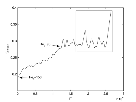
Figure 1: Time history of the mean flow rate relaminarization showing the initialization from $\mathrm{Re}_{\tau}=150$ to $\mathrm{Re}_{\tau}=95$. The window shows where data was collected.

Figure 2: Time history of the mean flow rate relaminarization for $\mathrm{Re}_{\tau}=95$. Three chugging cycles are seen near $t^{+}=2000,4000$ and $6000$ with the final relaminarization starting near $t^{+}=8000$.

The grid resolution was kept the same as for the original $\mathrm{Re}_{\tau}=150$ case. Thus the grid is effectively further refined to $\Delta r^{+}\approx 0.49$ and $(R\Delta\theta)^{+}\approx 3.1$ near the wall and $\Delta^{+}\approx 2.0$ near the centerline with a constant streamwise resolution of $\Delta z^{+}=4.0$, where $r$, $\theta$, and $z$ is the radial, azimuthal, and streamwise direction, respectively, and $R$ is the radius of the pipe.

III RESULTS

The profile of the mean flow with respect to wall units is seen in Figure 3. At this low Reynolds number, the profile does not conform to the log layer, yet near the wall it still exhibits a linear sublayer. Also, the flow does not conform to the laminar parabolic profile, indicating that it is indeed turbulent.

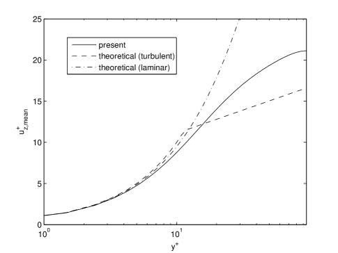
Figure 3: Mean flow profile versus $y^{+}=(1-r)\mathrm{Re}_{\tau}$ including the theoretical turbulent profile (dashed) with the sublayer ($u^{+}=y^{+}$), the log layer ($u^{+}=\log(y^{+})/0.41+5.5$), and the analytical parabolic laminar solution (dash-dot). The mean flow profile follows the law of the wall, yet deviates drastically from the log layer as expected.

The root-mean-square (rms) velocity profiles also show a turbulent trend as seen in Figure 4, although in comparison to the $\mathrm{Re}_{\tau}=150$ flow, the radial and azimuthal fluctuations are about half as strong, and the peak streamwise rms velocity is shifted further away from the wall. Also noteworthy is the strong fluctuations near the center of the pipe at $y^{+}\approx 90$. This is the first indication that the dynamics near the center of the pipe differ from what is expected for the fully turbulent case.

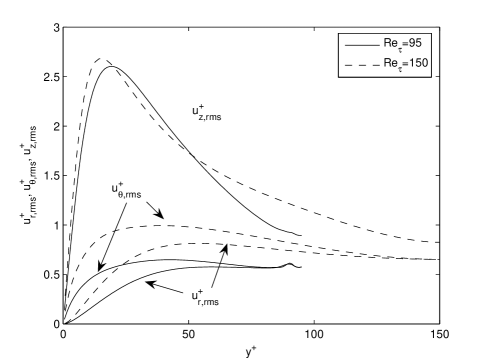
Figure 4: Root-mean-squared velocity profiles for $\mathrm{Re}_{\tau}=95$ (solid) and $\mathrm{Re}_{\tau}=150$ (dashed) versus wall units $y^{+}$. The inflections near $y^{+}=90$ are effects of the laminar chugging, because the rms velocities are averaged over all time steps.

The Reynolds stress profile also differs from the $\mathrm{Re}_{\tau}=150$ case and is shown in Figure 5. The Reynolds stress for the $\mathrm{Re}_{\tau}=95$ case has roughly half the magnitude throughout the radial profile, although the peak Reynolds stress is also found at the same location of $y^{+}=31$. The largest deviation from the expected profile occurs near the centerline beyond $y^{+}\approx 60$, where the Reynolds stress begins to fluctuate. In particular, between $y^{+}=88$ and $92$, the Reynolds stress is negative, which is physically interpreted as turbulence damping. Now, in addition to the rms deviation near the centerline, this Reynolds stress fluctuation indicates that the relaminarization process begins at the center of the pipe and goes towards the wall.

Figure 5: Reynolds stress profiles for $\mathrm{Re}_{\tau}=95$ (solid) and $\mathrm{Re}_{\tau}=150$ (dashed) versus wall units $y^{+}$. As in the rms velocity profiles, the inflections near $y^{+}=90$ are effects of the laminar chugging, showing that relaminarization begins at the center of the pipe.

Turning from statistics to the KL decomposition, we find that the chaotic attractor is reduced in size, as expected with a reduction in $\mathrm{Re}_{\tau}$, from $D_{KL}=2453$ to $D_{KL}=66$, shown in Figure 6. This dimension is similar to that found in Part I where the oscillated pipe was barely turbulent with a dimension of $D_{KL}=102$, and any stronger oscillation would have resulted in relaminarization.

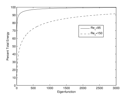
Figure 6: Comparison of the running total energy retained in the KL expansion for $\mathrm{Re}_{\tau}=95$ (solid) and $\mathrm{Re}_{\tau}=150$ (dashed). The 90% crossover point contains 2453 and 66 modes respectively, showing a drastic reduction in the turbulent attractor.

In observing the energy content of the modes in Table 1, and the most increased and decreased in Table 2, we find that the shear modes increase drastically, which is a result of the chugging motion and large mean flow rate fluctuations. Also of note is the increase in strength of the $n=3,4$ and $5$ streamwise vortices $(m=0)$ and their associated wall traveling waves $(m=1)$. The increase in the $(0,1,1)$ and $(1,0,1)$ modes, since they are not found in the work by Kerswell kerswell and Faisst and Eckhardt, faisst could be the catalysts of energy triads in equations 1 and 2 between the $n=3,4$ and $5$ rolls and the wall traveling waves. For example, the $(1,3,1)$ and $(1,4,1)$ waves interact through the $(0,1,1)$ catalyst, and the $(1,3,1)$ wave and the $(0,3,1)$ roll interact through the $(1,0,1)$ catalyst. The modes that decreased the most in energy are more of a result of the lower Reynolds number, as the high modes $n=8,9$ and $10$ in the $\mathrm{Re}_{\tau}=150$ case were an important basis for streamwise vortices that were $94-117$ wall units apart. However, at $\mathrm{Re}_{\tau}=95$, these represent spacings of $60-75$ wall units, which is too small, thus explaining their drop in energy.

Table 1: Comparison of first 25 eigenvalues. $m$ is the streamwise wavenumber, $n$ is the spanwise wavenumber, and $q$ is the eigenvalue quantum number.

	$\mathrm{Re}_{\tau}=150$						$\mathrm{Re}_{\tau}=95$
Index	$m$	$n$	$q$	Energy	% Total		$m$	$n$	$q$	Energy	% Total
1	0	6	1	1.61	2.42%		0	0	1	114	55.76%
2	0	5	1	1.48	2.22%		0	3	1	9.63	4.72%
3	0	3	1	1.45	2.17%		0	4	1	8.39	4.11%
4	0	4	1	1.29	1.93%		0	1	1	7.79	3.82%
5	0	2	1	1.26	1.88%		0	2	1	6.30	3.09%
6	1	5	1	0.936	1.40%		0	0	2	5.98	2.93%
7	1	6	1	0.917	1.37%		0	5	1	2.79	1.37%
8	1	3	1	0.902	1.35%		1	4	1	2.18	1.07%
9	1	4	1	0.822	1.23%		1	3	1	1.85	0.90%
10	0	1	1	0.805	1.20%		0	0	3	1.83	0.90%
11	1	7	1	0.763	1.14%		0	6	1	1.56	0.77%
12	1	2	1	0.683	1.02%		1	5	1	1.45	0.71%
13	0	7	1	0.646	0.97%		1	2	1	1.42	0.70%
14	2	4	1	0.618	0.92%		0	1	2	1.34	0.66%
15	0	8	1	0.601	0.90%		1	0	1	1.30	0.64%
16	2	5	1	0.580	0.87%		1	6	1	0.884	0.43%
17	1	1	1	0.567	0.85%		1	1	1	0.815	0.40%
18	2	7	1	0.524	0.78%		0	7	1	0.727	0.36%
19	1	8	1	0.483	0.72%		2	4	1	0.716	0.35%
20	2	6	1	0.476	0.71%		2	3	1	0.665	0.33%
21	2	3	1	0.454	0.68%		2	5	1	0.589	0.29%
22	2	2	1	0.421	0.63%		2	2	1	0.544	0.27%
23	2	8	1	0.375	0.56%		0	2	2	0.521	0.26%
24	1	9	1	0.358	0.54%		2	6	1	0.487	0.24%
25	3	4	1	0.354	0.53%		1	1	2	0.479	0.23%

Table 2: Ranking of eigenfunctions by energy change between the $\mathrm{Re}_{\tau}=150$ and $\mathrm{Re}_{\tau}=95$ cases. $m$ is the streamwise wavenumber, $n$ is the spanwise wavenumber, and $q$ is the eigenvalue quantum number. The shear modes $(0,0,q)$ are among the most increased, as are the $n=3,4,$and $5$ rolls $(m=0)$ and wall modes $(m=1)$.

	Increase					Decrease
Rank	$\Delta\lambda_{\mathbf{k}}$	$m$	$n$	$q$		$\Delta\lambda_{\mathbf{k}}$	$m$	$n$	$q$
1	113.4	0	0	1		-0.399	1	7	1
2	8.18	0	3	1		-0.300	0	8	1
3	7.10	0	4	1		-0.241	1	8	1
4	6.99	0	1	1		-0.236	2	7	1
5	5.81	0	0	2		-0.229	1	9	1
6	5.04	0	2	1		-0.225	2	8	1
7	1.71	0	0	3		-0.186	0	9	1
8	1.36	1	4	1		-0.175	3	9	1
9	1.30	0	5	1		-0.173	3	8	1
10	1.12	0	1	2		-0.170	2	9	1
11	1.09	1	0	1		-0.165	1	10	1
12	0.94	1	3	1		-0.149	0	10	1

Looking at the normal speed locus in Figure 7, the modes for a wave packet similar to that of $\mathrm{Re}_{\tau}=150$, but with a slightly faster advection speed of $8.64$ versus $8.41$. This shows a Reynolds number dependence on the advection speed, as expected, since the advection speed was shown to scale with the mean flow rate when the flow rate was increased in part I with spanwise wall oscillation.

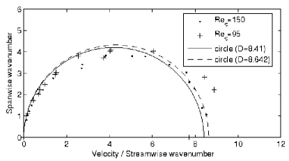
Figure 7: Comparison of normal speed locus for the $\mathrm{Re}_{\tau}=95$ ($\cdot$) and $\mathrm{Re}_{\tau}=150$ ($+$) cases. The solid lines represent a circle of diameter 8.41 and 8.64 respectively that intersect at the origin.

In visualizing the most energetic modes, the same structures as those found in the $\mathrm{Re}_{\tau}=150$ case are present. Figures 8 - 13 show the coherent vorticity for the most energetic modes for each of the subclasses discussed in part I. Since the $(0,0,1)$ mode has no coherent vorticity, the velocity is shown. Here we use “coherent vorticity” to refer to the imaginary eigenvalues of the velocity gradient tensor as defined in Chong et al. (also know as “degree of swirl”). chong Although slight differences are visible due to the lower Reynolds number, the same trends and characteristics are found for the KL modes as those found in the $\mathrm{Re}_{\tau}=150$ case.

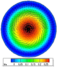
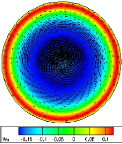
Figure 8: The (0,0,1) shear mode with contours of streamwise velocity and vectors of cross-stream velocities. Left: (a) $\mathrm{Re}_{\tau}=95$. Right: (b) $\mathrm{Re}_{\tau}=150$.

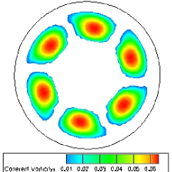
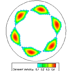
Figure 9: The (0,3,1) roll mode with contours of coherent vorticity. Left: (a) $\mathrm{Re}_{\tau}=95$. Right: (b) $\mathrm{Re}_{\tau}=150$.

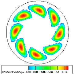
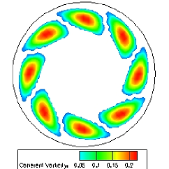
Figure 10: The (1,4,1) wall mode with contours of coherent vorticity. Left: (a) $\mathrm{Re}_{\tau}=95$. Right: (b) $\mathrm{Re}_{\tau}=150$.

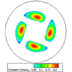
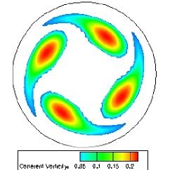
Figure 11: The (3,2,1) lift mode with contours of coherent vorticity. Left: (a) $\mathrm{Re}_{\tau}=95$. Right: (b) $\mathrm{Re}_{\tau}=150$.

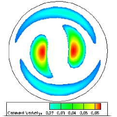
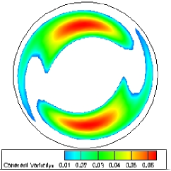
Figure 12: The (1,1,1) asymmetric mode with contours of coherent vorticity. Left: (a) $\mathrm{Re}_{\tau}=95$. Right: (b) $\mathrm{Re}_{\tau}=150$.

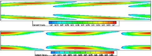
Figure 13: The (1,0,1) ring mode ($r$-$z$ plane cross-section) with contours of coherent vorticity. top: (a) $\mathrm{Re}_{\tau}=95$. Bottom: (b) $\mathrm{Re}_{\tau}=150$.

IV DYNAMICS

Recreating the time history of the KL modes reveals the interaction between the shear modes, roll modes, and propagating waves. As shown in Figure 16, the chugging phenomena happens when the propagating modes drop in energy. This happens at times $t^{+}\approx 1600$, $t^{+}\approx 3500$, and $t^{+}\approx 5500$, and starts the chugging phenomena. At $t^{+}\approx 8000$, the propagating modes drop too far in energy, and the flow relaminarizes. The chugging cycle ends again when the propagating waves spike at $t^{+}\approx 2200$, $t^{+}\approx 4100$, and $t^{+}\approx 6200$.

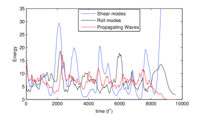
Figure 14: Time history of energy of shear modes (blue), roll modes (black), and propagating waves (red).

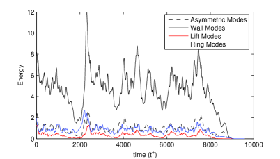
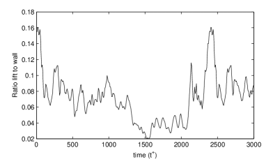
Figure 15: Time history of energy of propagating subclasses. Wall (solid black), lift (red), asymmetric (dashed), and rings (blue).

Figure 16: Ratio of lift mode energy to wall mode energy as a function of time. As the lift mode energy decreases with respect to the wall mode energy, relaminarization begins.

Examining the propagating waves based upon their subclass, shown in Figure 16, we find that the asymmetric and ring modes stay about the same energy as each other throughout the chugging cycles, while the wall modes are about a factor of 4 times more energetic. The lift modes, on the other hand, vary greatly in energy. When the lift modes decay from high to low energy, this coincides with the start of a chugging cycle, and ends when the lift modes regain the high energy state. This is emphasized in Figure 16 where the ratio of the lift mode total energy to the wall mode total energy is shown. In Figure 19, only one chug is shown, emphasizing the importance of the lift to wall ratio, and also the energy transfer between classes as energy flows from the rolls to the wall modes (through the ring modes), and then from the wall modes

Figure 17: Time history of energy of subclasses for a single chug. From the top: the mean velocity, roll mode energy, ring mode energy, wall mode energy, asymmetric mode energy, lift mode energy, and the lift to wall mode energy ratio. The start of the chug (blue dashed line) is when the lift to wall mode energy ratio drops too low. The end of the chug (red dashed line) is when the ratio spikes and recovers. The phase lag in energy from the roll to the wall modes (through the ring modes) and similarly from the wall to the lift modes (primarily through the asymmetric modes) can be seen.

Figure 18: Average energy spectra of the propagating modes. Wall (solid), lift (dashed), asymmetric (dots), and rings (dash-dot). Figure 19: Time history of the energy spectra of the propagating modes. $t^{+}=0$ and $t^{+}=2392$ show the proper established energy spectra at the beginning of the simulation, and well after the chug. $t^{+}=1592$ is the spectra when the chug begins. $t^{+}=2112,2552$ and $2232$ show the spectra regaining strength with time, finishing the chug cycle. Like the dynamics of the lift to wall energy ratio, the chugging spectra reinforces the dependence of the self-sustaining mechanism of wall turbulence on the high frequencies found in the inertial range, represented by the lift modes.

to the lift modes (primarily through the asymmetric modes).

Observing the energy spectra throughout the chug, we first revisit the total energy distribution of the propagating waves as averaged over the entire flow, seen in Figure 19. Again, like the $\mathrm{Re}_{\tau}=150$ spectrum, the lift modes are more energetic than the wall modes for high wavenumbers. Thus, because the high wavenumbers of the spectra dies off by two orders of magnitude at the start of the chug cycle, seen in Figure 19, it reinforces the importance of the lift modes in maintaining the turbulent flow.

As noted in the $\mathrm{Re}_{\tau}=150$ case, the lift modes are responsible for the majority of turbulence near the center of the pipe, as the wall modes stay near the wall, even for high quantum number. Thus, the importance of the outer region in the self sustaining mechanism of turbulence is reinforced. If the lift modes do not receive enough energy, cascaded through the wall modes, the relaminarization process begins near the center of the pipe. This is confirmed by the presence of the large drop in the rms velocities and Reynolds stress profiles near the center of the pipe. If the process cannot be halted in time by the transfer of energy from the wall modes to the lift modes, typically through the (1,3,1) or (1,4,1) modes, the flow will completely relaminarize. Adding in the findings of triad interactions by Webber et al., webber2 the flow of energy is shown in Figure 20. The shear to roll interactions are catalyzed by the rolls themselves, the roll to wall interactions are catalyzed mostly by the ring modes, and the wall to lift modes are catalyzed by both the ring and the asymmetric modes, and other lift modes. In the relaminarization process, it is this final leg that fails, breaking the mechanism, and starting relaminarization from the center of the pipe.

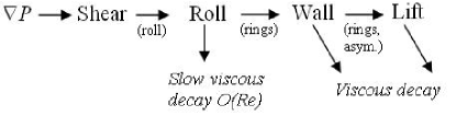
Figure 20: Energy flow chart for turbulence subclasses with catalysts. If any of these legs are disrupted, turbulence reduction (or drag reduction) begins. For instance, in Part I the energy in the wall modes were reduced by lifting them off the wall by spanwise wall oscillations, reducing their energy by forcing them to advect faster and died faster. In the current relaminarization case, not enough energy is present to fully populate the lift modes, and so their energy decreases and again the energy balance is disrupted.

V CONCLUSIONS

It is apparent through the examination of the spanwise wall oscillated case in Part I and the relaminarization case in Part II that if any leg of the energy cycle in a turbulent flow is disrupted, the resulting imbalance can lead to the start of a relaminarization process, and even complete relaminarization. In Part I, we describe a model where the propagating wall modes were pushed to higher advection speeds, reducing their effective lifespan. Thus they do not have enough time to take energy from the roll modes, breaking the third leg of the mechanism. Here in Part II, with lower pressure gradient, there is not enough energy to properly maintain the lift modes, and the last leg of the process is broken, starting the relaminarization process.

Thus, in conclusion, we find that while the wall modes and near wall interactions are responsible for the generation of turbulence from the pressure gradient, the turbulence in the outer region is necessary to maintain the proper inertial range in the energy spectra, and that without it, the relaminarization process begins.

References

- (1) A. Duggleby, K. S. Ball, and M. R. Paul, “Dynamics of propagating turbulent pipe flow structures. Part I: Effect of drag reduction by spanwise wall oscillation”, Phys. Fluids (2006), submitted. ArXiv:physics/0608258 http://lanl.arxiv.org/pdf/physics/0608258.
- (2) A. Talamelli, N. Fornaciari, K. J. A. Westin, and P. H. Alfredsson, “Experimental investigation of streaky structures in a relaminarizing boundary layer”, J. Turb. 18 (2002).
- (3) H. H. Fernholz and D. Warnack, “The effecs of a favourable pressure gradient and of the Reynolds number on an incompressible axisymmetric turbulent boundary layer. Part II. the turbulent boundary layer”, J. Fluid Mech. 359, 327–356 (1998).
- (4) H. H. Fernholz and D. Warnack, “The effecs of a favourable pressure gradient and of the Reynolds number on an incompressible axisymmetric turbulent boundary layer. Part I. the boundary layer with relaminarization”, J. Fluid Mech. 359, 357–381 (1998).
- (5) D. Greenblatt and E. A. Moss, “Rapid temporal acceleration of a turbulent pipe flow”, J. Fluid Mech. 514, 327–350 (2004).
- (6) J. Peixinho and T. Mullin, “Decay of turbulence in pipe flow”, Phys. Rev. Lett. 96 (2006).
- (7) K. Nakabayashi, W. Sha, and Y. Tsuchida, “Relaminarization phenomena and external-disturbance effects in spherical Couette flow”, J. Fluid Mech. 534, 327–350 (2005).
- (8) M. Hogerg, T. R. Bewley, and D. S. Henningson, “Relaminarization of =100 turbulence using gain scheduling and linear state-feedback control”, Phys. of Fluids 15, 3572–3575 (2003).
- (9) R. R. Kerswell, “Recent progress in understanding the transition to turbulence in a pipe”, Nonlinearity 18, R17–R44 (2005).
- (10) H. Faisst and B. Eckhardt, “Traveling waves in pipe flow”, Phys. Rev. Lett. 91 (2003).
- (11) A. Duggleby, K. S. Ball, M. R. Paul, and P. F. Fischer, “Dynamical eigenfunction decomposition of turbulent pipe flow”, J. of Turbulence (2006), submitted. ArXiv:physics/0608257, http://lanl.arxiv.org/pdf/physics/0608257.
- (12) G. A. Webber, R. A. Handler, and L. Sirovich, “Energy dynamics in a turbulent channel flow using the Karhunen-Loève approach”, Int. J. Numer. Meth. Fluids 40, 1381–1400 (2002).
- (13) M. S. Chong, A. E. Perry, and B. J. Cantwell, “A general classification of three-dimensional flow fields”, Phys. Fluids A 2, 765–777 (1990).