Dynamical Eigenfunction Decomposition of
Turbulent Pipe Flow

Abstract

The results of an analysis of turbulent pipe flow based on a Karhunen-Loève decomposition are presented. The turbulent flow is generated by a direct numerical simulation of the Navier-Stokes equations using a spectral element algorithm at a Reynolds number Re${}_{\tau}=150$. This simulation yields a set of basis functions that captures 90% of the energy after 2,453 modes. The eigenfunctions are categorised into two classes and six subclasses based on their wavenumber and coherent vorticity structure. Of the total energy, 81% is in the propagating class, characterised by constant phase speeds; the remaining energy is found in the non propagating subclasses, the shear and roll modes. The four subclasses of the propagating modes are the wall, lift, asymmetric, and ring modes. The wall modes display coherent vorticity structures near the wall, the lift modes display coherent vorticity structures that lift away from the wall, the asymmetric modes break the symmetry about the axis, and the ring modes display rings of coherent vorticity. Together, the propagating modes form a wave packet, as found from a circular normal speed locus. The energy transfer mechanism in the flow is a four step process. The process begins with energy being transferred from mean flow to the shear modes, then to the roll modes. Energy is then transfer ed from the roll modes to the wall modes, and then eventually to the lift modes. The ring and asymmetric modes act as catalysts that aid in this four step energy transfer. Physically, this mechanism shows how the energy in the flow starts at the wall and then propagates into the outer layer.

1 Introduction

Turbulence, hailed as one of the last major unsolved problems of classical physics, has been the subject of numerous publications as researchers seek to understand the underlying physics, structures, and mechanisms inherent to the flow [1]. The standard test problem for wall-bounded studies historically has been turbulent channel flow because of its simple geometry and computational efficiency. Even though much insight has been achieved through the study of turbulent channel flow, it remains an academic problem because of its infinite (computationally periodic) spanwise direction.

The next simplest geometry is turbulent pipe flow, which is of interest because of its real-world applications and its slightly different dynamics. The three major differences between turbulent pipe and channel flow are that pipe flow displays a log layer, but overshoots the theoretical profile until a much higher Reynolds numbers ($\mathrm{Re}=3000$ for a channel versus $\mathrm{Re}=7442$ for a pipe [2, 3]), has an observed higher critical Reynolds number, and is linearly stable to an infinitesimal disturbance [4, 5]. Unfortunately, few direct numerical simulations of turbulent pipe flow have been carried out because of the complexity in handling the numerical radial singularity at the origin. Although the singularity itself is avoidable, its presence causes standard high-order spectral methods to fail to converge exponentially. As a result, only a handful of algorithms found in the literature for turbulent pipe flow; the first reported use for each algorithm is listed in Table 1. These algorithms typically use a low-order expansion in the radial direction. Only Shan et al. [6] using concentric Chebyshev domains (“piecemeal”) and Loulou et al. [7] using basis spline (B-spline) polynomials provide a higher-order examination of turbulent pipe flow. Using a spectral element method, this study provides not only a high-order examination but the first exponentially convergent investigation of turbulent pipe flow through direct numerical simulation (DNS).

Summary of existing algorithms for the DNS of turbulent pipe flow, citing the first reported use for each algorithm. As seen, most approaches use a 2nd-order radial discretization. The reason is that the standard spectral methods, in the presence of the coordinate singularity, achieve only 2nd-order convergence instead of geometric convergence. Authors Radial Discretization Eggels et al. (1994) [8] 2nd-order FD - first pipe DNS Verzicco and Orlandi (1996) [9] 2nd-order FD flux based Fukagata and Kasagi (2000) [10] 2nd order FD - energy conservative Shan et al. (1999) [6] “Piecemeal” Chebyshev Loulou et al.(1997) [7] B-spline

With this DNS result, one of the studies that can be performed with the full flow field and time history it provides is an analysis based on an orthogonal decomposition method. In such methods, the flow is expanded in terms of a natural or preferred turbulent basis. One method used frequently in the field of turbulence is Karhunen-Loève (KL) decomposition, which uses a two-point spatial correlation tensor to generate the eigenfunctions of the flow. This is sometimes referred to as proper orthogonal decomposition, empirical orthogonal function, or empirical eigenfunction analysis.

Work in this area was pioneered by Lumley, who was the first to use the KL method in homogeneous turbulence [11, 12]. This method was later applied to turbulent channel flow in a series of papers by Ball, Sirovich, and Keefe [13, 14] and Sirovich, Ball, and Handler [15], who discovered plane waves and propagating structures that play an essential role in the production of turbulence through bursting or sweeping events. To study the interactions of the propagating structures, researchers have examined minimal expansions of a turbulent flow [16, 17, 18, 19]. These efforts have led to recent work by Webber et al. [20, 21], who examined the energy dynamics between KL modes and discovered the energy transfer path from the applied pressure gradient to the flow through triad interactions of KL modes.

This present study uses a spectral element Navier-Stokes solver to generate a globally high-order turbulent pipe flow data set. The Karhunen-Loève method is used to examine the turbulent flow structures and dynamics of turbulent pipe flow.

2 Methodology

The direct numerical simulation of the three-dimensional time dependent Navier-Stokes equations is a computationally intensive task. By fully resolving the necessary time and spatial scales of turbulent flow, however, no subgrid dissipation model is needed, and thus a turbulent flow is calculated directly from the equations. DNS has one main advantage over experiments, in that the whole flow field and time history are known, enabling analyses such as the Karhunen-Loève decomposition.

Because of the long time integration and the grid resolution necessary for DNS, a high-order (typically spectral) method is often used to keep numerical round-off and dissipation error small. Spectral methods and spectral elements use trial functions that are infinitely and analytically differentiable to span the element. This approach decreases the global error exponentially with respect to resolution, in contrast to an algebraic decrease with standard methods such as finite difference or finite element methods [22].

2.1 Direct Numerical Simulation

2.1.1 Numerical Methods

This study uses a spectral element Navier-Stokes solver that has been developed over the past 20 years [23, 24] to solve the Navier-Stokes equations:

$$\partial_{t}\mathbf{U}+\mathbf{U}\cdot\nabla\mathbf{U}=-\nabla P+\mathrm{Re}_{\tau}^{-1}\nabla^{2}\mathbf{U}$$ (1)

$$\nabla\cdot\mathbf{U}=0.$$ (2)

In the above equations, $\mathbf{U}=(U_{r},U_{\theta},U_{z})$ is the velocity vector corresponding to the radial, azimuthal, and streamwise direction respectively; Re${}_{\tau}=U_{\tau}R/\nu$ is the Reynolds number; $R$ is the radius of the pipe; $\nu$ is the kinematic viscosity; and $U_{\tau}=\sqrt{\tau_{w}/\rho}$ is the shear velocity based upon the wall shear stress $\tau_{w}$ and density $\rho$. This solver employs a geometrically flexible yet exponentially convergent spectral element discretization in space, in this case allowing the geometry to be fitted to a cylinder. The domain is subdivided into elements, each containing high-order (usually 11–13) Legendre Lagrangian interpolants. The resulting data localisation allows for minimal communication between elements, and therefore efficient parallelization. Time discretization is done with third-order operator splitting methods, and the remaining tensor-product polynomial bases are solved by using conjugate gradient iteration with scalable Jacobi and hybrid Schwarz/multigrid preconditioning [25].

2.1.2 Geometry

Spectral elements are effective in cylindrical geometries [26] and their use elegantly avoids the radial singularity at the origin. The mesh is structured as a box near the origin and transitions to a circle near the pipe walls (Figure 1), maintaining a globally high-order method at both the wall and the origin. In addition to avoiding the numerical error associated with the singularity, the method also avoids the time-step restriction due to the smaller element width at the origin of a polar-cylindrical coordinate system, which could lead to potential violations of the Courant-Friedrichs-Levy stability criteria.

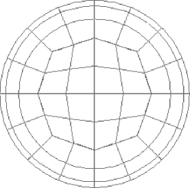
Figure 1: Cross section of the spectral element grid for pipe flow. The spectral element algorithm avoids the singularity found in polar cylindrical coordinates.

Each slice, as shown in Figure 1, has 64 elements, and there are 40 slices stacked in the streamwise direction, adding up to a length of 20R. Each element has 12th-order Legendre polynomials in each direction for Re${}_{\tau}=150$. This discretization results in 4.4 million degrees of freedom. Near the wall, the grid spacing normalised by wall units ($\nu/U_{\tau}$) denoted by the superscript ⁺ is $\Delta r^{+}\approx 0.78$ and $(R\Delta\theta)^{+}\approx 4.9$, where $r$ is the radius and $\theta$ is the azimuthal angle. Near the centre of the pipe, the spacing in Cartesian coordinates is $\Delta^{+}\approx 3.1$. The streamwise grid spacing is a constant $\Delta z^{+}=6.25$ throughout the domain where $z$ is the streamwise coordinate.

2.1.3 Benchmarking at $\mathrm{Re}_{\tau}=180$

Benchmarking was performed at Re${}_{\tau}=180$ with the experiments and DNS of Eggels et al. [8] and the DNS of Fukagata and Kasagi [10]. For this higher Reynolds number flow, 14th-order polynomials were used, giving grid spacings near the wall of $\Delta r^{+}\approx 0.80$ and $(R\Delta\theta)^{+}\approx 5.0$, $\Delta^{+}\approx 3.2$ in the centre, and $\Delta z^{+}=6.42$. Eggels et al. and Fukagata and Kasagi used a spectral Fourier discretization in the azimuthal and axial directions and then a 2nd-order finite difference discretization in the radial direction. Also, both groups used a domain length of 10R and grid sizes in their DNS studies of $96\times 128\times 256$ for $r$, $\theta$, and $z$ directions, respectively.

The turbulent flow was tripped with a solenoidal disturbance, and the simulation was run until transition was complete. This was estimated by examining the mean flow and root-mean-squared statistics over sequential periods of 100 $t^{+}$ until a statistically steady state was achieved, marked by a change of less than 1 percent between the current and previous period. In this case, it took $7000t^{+}$ to arrive at a statistically steady state. Convergence was checked by examining the total fluctuating energy after 1000 time steps for increasing polynomial orders 8, 10, 12, and 14 with a fixed number of elements (2560). The absolute value of the difference of the total fluctuating energy for each simulation and the value obtained using 16th order polynomials was plotted versus the total number of degrees of freedom in Figure 2. The exponential decay of the error with increasing degrees of freedom shows that our spectral element algorithm achieves geometric or exponential convergence.

Figure 2: Convergence plot showing the error in fluctuating total energy of the flow versus degrees of freedom after 1000 time steps for a fixed grid and polynomial orders of 8, 10, 12, and 14 (circles), using 16th order polynomials to approximate the exact solution. The exponentially decay of the curve fit (solid) shows that our spectral element algorithm is geometrically or exponential convergent.

The mean flow profiles in Figure 3 correspond well with the hot wire anemometry (HWA) results of Eggels et al. [8], but as seen in the root-mean-squared (rms) statistics shown in Figure 4, the spectral element calculation shows a lower peak $U_{z,rms}$ and higher peak $U_{\theta,rms}$ and $U_{r,rms}$ compared to the HWA, particle image velocimetry (PIV), and laser Doppler anemometry (LDA) results. These results are in contrast to those with channel flow, as reported by Gullbrand [27], where the 2nd order finite difference methods undershoot the spectral method wall-normal velocity rms.

When compared to the experimental results of Eggels et al. [8], the spectral element results are in better agreement than the 2nd-order finite difference results. We note that Eggels et al. report that their (PIV) system had difficulties capturing $U_{r}$ near the wall and near the centerline of the pipe due to reflection, which could explain the deviation of all of the DNS results in that area.

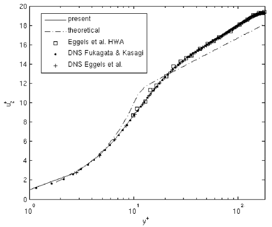
Figure 3: Benchmark of mean velocity profile for the spectral element algorithm vs low-order methods of Eggels et al.[8] and Fukagata and Kasagi [10] for Re${}_{\tau}=180$. The theoretical line is the law of the wall $U^{+}=y^{+}$ and the log layer $U^{+}=1/0.41\log y^{+}+5.5$. Deviations from the log layer are expected in turbulent pipe flow until much higher Reynolds numbers.

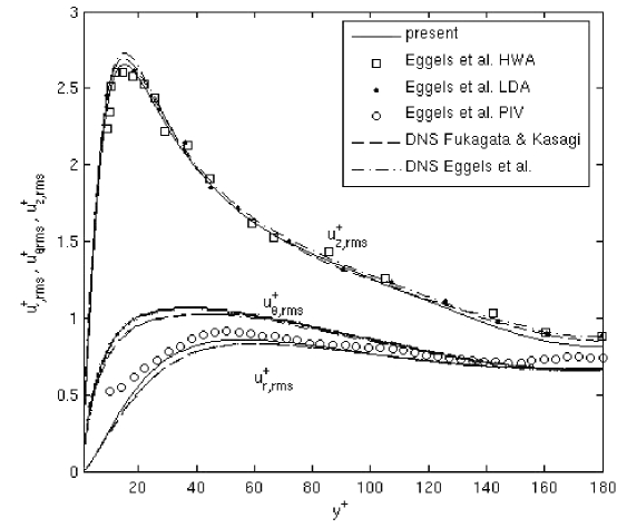
Figure 4: Benchmark of the rms profiles for Re_τ=180 comparing the spectral element algorithm vs the low-order methods of Eggels et al.[8] and Fukagata and Kasagi [10]. As seen near $y^{+}=20$ in the $u^{+}_{z,rms}$ and near $y^{+}=50$ in the $u_{r,rms}^{+}$, the higher-order method is closer to the experimental results than the 2nd-order methods.

A second major difference our spectral element method and the previous pipe DNS using 2nd-order finite difference is the domain size. With the spectral element method, which results in a global high-order convergence, a domain size of 10R yielded unphysical results in the flow, as seen in the bulge in the azimuthal $U_{\theta,rms}$ in Figure 5 at $y^{+}=55$ and $y^{+}=120$. This unphysical result arose even with a more refined grid, and is therefore not a function of under-resolution. However, when the domain of the spectral element method was extended to 20R, this problem disappeared. We surmise that the 2nd-order finite difference method dissipated some large-scale structures after 10R that the higher-order spectral element case appropriately resolves. This undissipated structure, because of the periodic boundary conditions, then re-enters the inlet and causes the unphysical bulges in the azimuthal rms profile. This result is also supported by the work of Jiménez [28] in turbulent channel flow (Re_τ=180) that shows large-scale structures that extend well past the domain size of $z^{+}=1800=10R$.

This benchmark confirms that the spectral element algorithm, at the given grid resolution and domain size, will generate the appropriate turbulent flow field and time history to perform the KL decomposition.

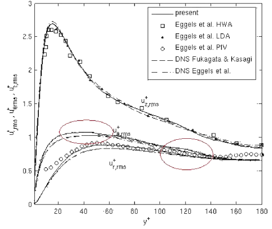
Figure 5: Effect of a short domain (10R) with a high-order method, showing unphysical deviations in the rms profiles near $y^{+}=50$ and $y^{+}=120$ for the spectral element algorithm for Re${}_{\tau}=180$. A bulge, highlighted by the red ovals, is present in the azimuthal rms that is not found in the low-order methods of Eggels et al.[8] and Fukagata and Kasagi [10]. By extending the domain to 20R, the unphysical bulge is removed. bfIt is therefore surmised that the unphysical result is possibly due to the more dissipative nature of the low-order schemes that washes away a long-scale structure that the present high-order scheme captures and re-enters the inlet from the periodic outflow conditions.

2.2 Karhunen-Loève Decomposition

For completeness, the Karhunen-Loève Decomposition method is briefly described here, but for more detail, see [13, 29, 30, 31, 32, 16, 15, 14, 11, 12].

2.2.1 Numerical Method

The Karhunen-Loève method is the solution of the two-point velocity correlation kernel equation defined by

$$\int_{0}^{L}\int_{0}^{2\pi}\int_{0}^{R}K(\mathbf{x},\mathbf{x^{\prime}})\mathbf{\Phi}(\mathbf{x}^{\prime})r^{\prime}dr^{\prime}d\theta^{\prime}dz^{\prime}=\lambda\mathbf{\Phi}$$ (3)

$$K(\mathbf{x},\mathbf{x^{\prime}})=\langle\mathbf{u}(\mathbf{x})\otimes\mathbf{u}(\mathbf{x^{\prime}})\rangle,$$ (4)

where $\mathbf{u}(\mathbf{x})=\mathbf{U}(\mathbf{x})-\overline{\mathbf{U}}(\mathbf{x})$ is the fluctuating component of the velocity and where the mean $\overline{\mathbf{U}}(\mathbf{x})$ is determined by averaging over both homogeneous planes and time. The angle brackets represent an average over many time steps, on the order of $t^{+}\approx 40,000\sim 50,000$, to sample the the entire attractor. The $\otimes$ denotes the outer product, establishing the kernel as the velocity two-point correlation between every spatial point $\mathbf{x}=(r,\theta,z)$ and $\mathbf{x^{\prime}}=(r^{\prime},\theta^{\prime},z^{\prime})$.

For turbulent pipe flow, with two homogeneous directions providing translational invariance in the $\theta$ (azimuthal) and $z$ (streamwise) direction, Eq. (4) becomes

$$K(\mathbf{x},\mathbf{x^{\prime}}) = K(r,r^{\prime},\theta-\theta^{\prime},z-z^{\prime})$$ (5)

$$= \mathcal{K}(n,m;r,r^{\prime})e^{in\theta}e^{i2\pi mz/L}.$$ (6)

Thus, given the kernel in Eq. (5), the eigenfunctions have the form

$$\mathbf{\Phi}_{(m,n)}(r,\theta,z)=\mathbf{\Psi}(n,m;r)e^{in\theta}e^{i2\pi mz/L},$$ (7)

where $n$ is the azimuthal wavenumber and $m$ the streamwise wavenumber. The determination of $\mathbf{\Psi}$ is then given by

$$\int_{0}^{R}\mathcal{K}(m,n;r,r^{\prime})\mathbf{\Psi}^{\star}(m,n;r^{\prime})r^{\prime}dr^{\prime}=\lambda_{mn}\mathbf{\Psi}(m,n;r),$$ (8)

$$\mathcal{K}(m,n;r,r^{\prime})=\langle\hat{\mathbf{u}}(n,m;r)\otimes\hat{\mathbf{u}}(n,m;r^{\prime})\rangle$$ (9)

where the $\star$ denotes the complex conjugate, $\lambda$ is the eigenvalue, and $\hat{\mathbf{u}}(n,m;r)$ is the Fourier transform of the fluctuating velocity in the azimuthal and axial direction.

In the present problem, 2,100 snapshots of the flow field were taken, corresponding to one snapshot every eight viscous time steps ( $t^{+}=U_{\tau}^{2}t/\nu$). The results of each snapshot were projected to an evenly spaced grid with $101\times 64\times 400$ points in $r,\theta,$ and $z$, respectively. The Fourier transform of the data was then taken and the kernel assembled. This kernel was averaged over every snapshot to generate the final kernel to be decomposed. Since the dimension of K is 303 (given by three velocity components on 101 radial grid points) there are 303 eigenfunctions and eigenvalues for each Fourier wavenumber pair $(m,n)$. The eigenfunctions are ranked in descending order with the quantum number $q$ to specify the particular eigenfunction associated with the corresponding eigenvalue. Thus, it requires a triplet $(m,n,q)$ to specify a given eigenfunction.

The eigenfunctions $\mathbf{\Psi}_{q}(m,n;r)$ are complex vector functions and are normalised so that the inner product of the full eigenfunction $\mathbf{\Phi}_{(m,n,q)}$ is of unit length, namely $(\mathbf{\Phi}_{(m,n,q)},\mathbf{\Phi}_{(n^{\prime},m^{\prime},q^{\prime})})=\delta_{mm^{\prime}}\delta_{nn^{\prime}}\delta_{qq^{\prime}}$, where $\delta$ is the Kronecker delta. The eigenvalues physically represent the average energy of the flow captured by the eigenfunction $\mathbf{\Phi}_{(m,n,q)}$,

$$\lambda_{(m,n,q)}=\langle|(\mathbf{u},\mathbf{\Phi}_{(m,n,q)})|^{2}\rangle.$$ (10)

We note that the eigenfunctions, as an orthogonal expansion of the flow field, retain the properties of the flow field, such as incompressibility and boundary conditions of no slip at the wall.

2.2.2 Symmetry Considerations

The pipe flow is statistically invariant under azimuthal reflection,

$$R_{\theta}:(r,\theta,z,u_{r},u_{\theta},u_{z})\rightarrow(r,-\theta,z,u_{r},-u_{\theta},u_{z}),$$ (11)

and taking advantage of it reduces the total number of calculations as well as the memory and storage requirements. We note that, because of its geometry, turbulent channel flow has two more symmetries – a vertical reflection, and a x-axis rotation – that are not present in the pipe, since a negative radius is equivalent to a 180 degree rotation in the azimuthal direction.

A major consequence of this symmetry is that the resulting eigenfunctions are also symmetric, and the modes with azimuthal wave number $n$ will be the azimuthal reflection of the modes with wave number $-n$,

$$R_{\theta}:(\Phi^{r}_{(m,n,q)},\Phi^{\theta}_{(m,n,q)},\Phi^{z}_{(m,n,q)})\rightarrow(\Phi^{r}_{(m,-n,q)},-\Phi^{\theta}_{(m,-n,q)},\Phi^{z}_{(m,-n,q)}),$$ (12)

thus reducing the total computational memory needed for this calculation.

2.2.3 Time-Dependent Eigenfunction Flow Field Expansion

The KL method provides an orthogonal set of eigenfunctions that span the flow field. As such, the method allows the flow field to be represented as an expansion in that basis,

$$\mathbf{u}(r,\theta,z,t)=\sum_{(m,n,q)}a_{(m,n,q)}(t)\mathbf{\Phi}_{(m,n,q)}(r,\theta,z),$$ (13)

with

$$a_{(m,n,q)}(t)=(\mathbf{\Phi}_{(m,n,q)}(r,\theta,z),\mathbf{u}(r,\theta,z,t)).$$ (14)

Since the Fourier modes are orthogonal to each other, equation 14 becomes

$$a_{(m,n,q)}(t)=2\pi L_{z}\int_{0}^{R}\mathbf{\Psi}_{q}(m,n;r)\mathbf{\hat{u}^{\star}}(m,n;r,t)rdr,$$ (15)

with $\mathbf{\hat{u}}$ being the Fourier transform of $\mathbf{u}$ in the azimuthal and streamwise direction with wavenumbers $n$ and $m$, respectively.

The time history of the eigenfunctions can be used to examine their interactions, such as the energy interaction examined by Webber et al. [21] and bursting events by Sirovich et al. [15].

3 Results

This section presents the results of our analysis of turbulent pipe flow based on KL decomposition.

3.1 Mean Properties of Flow and Flow Statistics

DNS was performed for $\mathrm{Re}_{\tau}=150$. The Reynolds number based on the centreline velocity is $\mathrm{Re}_{c}\approx 5700$ and based on the mean velocity is $\mathrm{Re}_{m}\approx 4300$. This range is above the observed critical Reynolds number for pipe flow and exhibits self-sustaining turbulence, as seen from the fluctuating time history of the mean velocity shown in Figure 6. The velocity profile, seen in Figure 7, shows the mean velocity with respect to wall units away from the wall ($y^{+}=(r-R)U_{\tau}/\nu$). The profile fits the law of the wall but fails to conform to the log law, and as mentioned in Section 1, the log law is not expected for turbulent pipe flow until much higher Reynolds number.

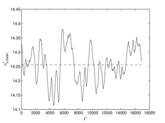
Figure 6: Variations in bulk mean velocity $u_{m}(t^{+})$ consistent with turbulent pipe flow. The dashed line is the time averaged mean velocity.

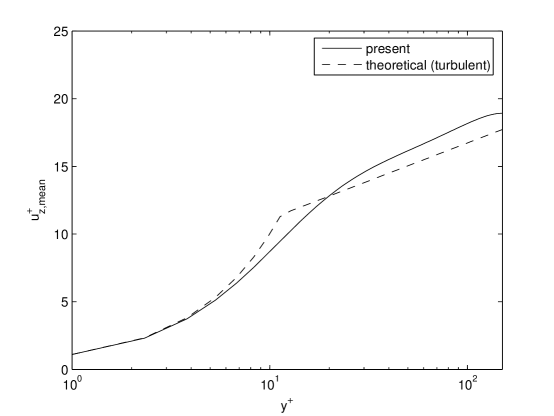
Figure 7: Mean velocity profile (solid) compared to the theoretical law of the wall $u^{+}=y^{+}$ and the log layer $u^{+}=1/0.41\log y^{+}+5.5$ (dashed). As in the Re${}_{\tau}=180$ case, the overshoot of the log layer above the theoretical profile is expected in turbulent pipe flow until much higher Reynolds number.

The rms velocity fluctuation profiles and the Reynolds stress profile is shown in Figures 8b and 8b. The streamwise fluctuations peak near $y^{+}=16$. The azimuthal and axial velocities show a weaker peak near $y^{+}=39$ and $y^{+}=55$, respectively, and then remain fairly flat throughout the pipe. The Reynolds stress $\overline{v_{z}v_{r}}$ has a maximum of 0.68 at $y^{+}=31$.

Figure 8a: Root-mean-square statistics across the pipe for the radial (solid), azimuthal (dashed), and streamwise (dot-dashed) velocities. The results show the standard profiles, similar to the Re${}_{\tau}=180$ rms profiles.

Figure 8b: Reynolds stress $\overline{v_{z}v_{r}}$ across the pipe (solid), peaking at 0.68 at $y^{+}=31$, and the total shear stress distribution (dashed).

3.2 Eigenvalue Spectrum

As discussed in Section 2.2, the eigenvalues represent the energy of each eigenfunction. By ordering the eigenvalues from largest to smallest, one can minimise the number of eigenfunctions, $N$, needed to capture a given percentage of the energy of the flow. Table 3.2 shows the first 25 eigenfunctions, and Figure 9 shows the running total of energy versus modes. The first mode to have $q\neq 1$ is the 41st mode (0,0,2). The 90% mark is reached at $D_{KL}=2,453$, where $D_{KL}$ can be considered as a measure of the intrinsic dimension of the chaotic attractor describing the turbulence as discussed by Zhou and Sirovich [32, 17]. These eigenfunctions are the preferred or natural basis function for turbulent pipe flow, and insight is gained by observing their qualitative structure.

First 25 eigenvalues ranked in descending order of energy. Index m n q Eigenvalue Energy (% Total) 1 0 6 1 1.61 2.42 % 2 0 5 1 1.48 2.22 % 3 0 3 1 1.45 2.17 % 4 0 4 1 1.29 1.93 % 5 0 2 1 1.26 1.88 % 6 1 5 1 0.936 1.40 % 7 1 6 1 0.917 1.37 % 8 1 3 1 0.902 1.35 % 9 1 4 1 0.822 1.23 % 10 0 1 1 0.805 1.20 % 11 1 7 1 0.763 1.14 % 12 1 2 1 0.683 1.02 % 13 0 7 1 0.646 0.97 % 14 2 4 1 0.618 0.92 % 15 0 8 1 0.601 0.90 % 16 2 5 1 0.580 0.87 % 17 1 1 1 0.567 0.85 % 18 2 7 1 0.524 0.78 % 19 1 8 1 0.483 0.72 % 20 2 6 1 0.476 0.71 % 21 2 3 1 0.454 0.68 % 22 2 2 1 0.421 0.63 % 23 2 8 1 0.375 0.56 % 24 1 9 1 0.358 0.54 % 25 3 4 1 0.354 0.53 %

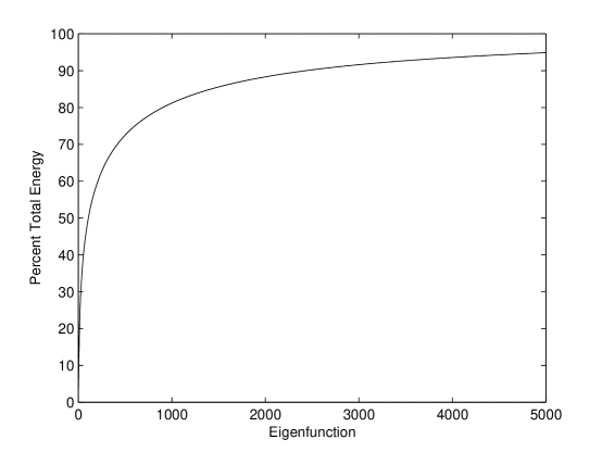
Figure 9: Percentage of energy retained in the KL expansion with the 90% mark achieved after 2453 modes (Karhunen-Loève dimension).

3.3 Structure of the Eigenfunctions

The eigenfunctions resulting from the KL decomposition can be categorised into two distinct classes and six sub-classes based on their characteristics, as listed in Table 3.3 and depicted in Figure 10. It is observed that certain characteristics of the eigenfunction are dependent on the wavenumber. The modes with higher azimuthal than axial wavenumber turn more than they lift, and as such the near-wall stretching structures are found. Likewise the modes with higher axial than azimuthal wavenumber lift more than they turn, and as such the lifting structures that extend from the near wall to the outer region are found.

Structures of turbulent pipe flow as classified by wavenumber. Structure Definition Energy Description Figure Propagating Modes (m,n,q), $m\not=0$ 80.58% Constant phase speed         (a) Wall $n>m$ 35.22% Structures that turn azimuthally Fig. 11g-f more than they lift axially found near wall.         (b) Lift $m\geq n,n>1$ 29.68% Structures that lift axially more Fig. 12g-f than they turn azimuthally, extend from near wall to outer region         (c) Asymmetry $n=1$ 9.09 % Structures that have non-zero radial and Fig. 13g-f azimuthal velocity, typically with coherent structures found in the outer region         (d) Ring $n=0$ 6.60% Ring-like structures in the outer region Fig. 14g-f Non-propagating Modes $(0,n,q)$ 19.42% Non-constant phase speed         (a) Roll mode $(0,n,q)$ $n\not=0$ 18.34% Near wall streamwise vortices Fig. 15g-f         (b) Shear mode $(0,0,q)$ 1.08% Non-zero centerline streamwise velocity Fig. 16d-d No coherent vorticity

This eigenfunction expansion, using both their structure and their time-dependent coefficients, provides a framework for further analysis and comparison and has led to understanding the mechanism of drag reduction by spanwise wall oscillation [36] and the mechanism of relaminarization [37].

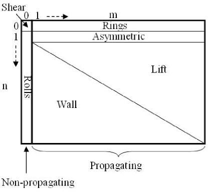
Figure 10: Subclass classification according to streamwise ($m$) and spanwise ($n$) wavenumbers.

In order to show the qualitative and quantitative classifications of these eigenfunctions, the most energetic function of each class is presented in Figures 11g through 16d. For each class, subfigures (a) show iso-contours and slices of coherent vorticity, and a slice displaying the Reynolds stress and coherent vorticity together. The coherent vorticity is defined as the rotating part of the fluid, defined as the imaginary component of the eigenvalues of the velocity strain rate tensor, following the work of Chong et al. [33]. The next four subfigures for each class are the plots of the eigenfunctions, both the real (b) and imaginary component (d), and the time history amplitude (c) and phase (e). To complete the class description, the coherent vorticity of two more representative eigenfunctions are shown in subfigures (f) and (g). For the shear modes (Figure 16d), since they do not have coherent vorticity, only the eigenfunction and time history are plotted.

The first subclass of interest is the wall eigenmodes. The coherent vorticity plots of three example wall modes are seen in Figures 11g, 11g, and 11g for the (1,5,1),(1,3,1), and (2,4,1) modes, respectively. Each mode consists of a travelling-wave coherent vortex near the wall, and all eigenmodes with greater spanwise wavenumber than streamwise wavenumber demonstrate this same structure. A characteristic consistent of this subclass is that the Reynolds stress is generated near the wall. The individual velocity components of the (1,2,1) mode, the most energetic wall mode, is shown in Figures 11g and 11g for their real and imaginary components, respectively, and in Figures 11g and 11g for their amplitude squared and phase time history. The amplitude history shows the bursting nature of these travelling-waves, and the near constant phase velocity shows why these modes are referred to as propagating or travelling-waves. These wall functions constitute 35.22% of the total energy of the flow, and are the most energetic of the propagating modes.

The next mode of interest, still in the propagating mode class, is the lift mode, found whenever the streamwise wavenumber is greater than or equal to the spanwise wavenumber and the spanwise wavenumber is greater than one. Three examples of this subclass are shown in Figures 12g, 12g, and 12g for modes (2,2,1), (3,2,1), and (3,3,1), respectively. In a lift mode, the coherent vorticity and Reynolds stress extends from the wall to near the centreline, and results in a lifting motion. The real and imaginary velocity components are shown in Figures 12g and 12g, respectively, and the amplitude and phase time history in Figures 12g and 12g, respectively. Again, the constant phase speed classifies these structures as propagating modes, and the amplitude bursts are also characteristic of a turbulent flow field. The lift structures constitute 29.68% of the total energy of the flow.

The next modes, the asymmetric modes, are responsible for breaking the symmetry of the flow about the axis of the pipe. These modes are found for a spanwise wavenumber of one, for any streamwise wavenumber, and consist of a coherent vortex just outside the log layer. They are asymmetric because of their nonzero radial and azimuthal velocities at the origin, which is physical only for azimuthal wavenumber $n=1$, since a positive radial velocity at the origin, under a rotation of $\pi$ around the axis, results in a negative radial velocity. The same is true for the azimuthal velocity at the origin. Three examples of these modes are shown in Figures 13g, 13g and 13g for modes (1,1,1), (2,1,1), and (3,1,1), respectively, again having the Reynolds stress between the coherent vorticity. These modes are also propagating and turbulent, as seen in the (1,1,1) mode’s amplitude (Figure 13g) and phase time history (Figure 13g), with its real and imaginary component found in Figure 13g and 13g. This mode constitutes 9.09% of the total energy of the flow.

The last of the propagating modes is the ring mode, named for the ring of coherent vorticity that is found for all modes with zero azimuthal wavenumber. Examples of this structure are shown in Figures 14g, 14g, and 14g for modes (1,0,1), (1,0,2), and (2,0,1), respectively. Since the ring modes have no azimuthal dependance, only a radial cross-section of coherent vorticity is shown with Reynolds stress superimposed. The real and imaginary velocities are shown in Figures 14g and 14g, and the amplitude and phase in 14g and 14g. This mode constitutes 6.60% of the total energy of the flow.

The last two modes are the non propagating modes. The first and more energetic of the two is the roll mode, found for any mode with zero streamwise wavenumber. This consists of rolls of coherent vorticity, as seen in the three example modes (0,6,1), (0,5,1), and (0,3,1) in Figures 15g, 15g, and 15g, respectively. The Reynolds stress is strong between the coherent vortices but is an order of magnitude less than those of the wall or lift structures. The velocity components of the (0,6,1) mode are shown in Figure 15g and 15g. Of note, these structures do not have a constant phase velocity, seen in Figure 15g, and the decay rate of the energy is slower than that of the propagating modes, seen if Figure 15g. This subclass constitutes 18.34% of the total energy of the flow.

The other non propagating mode is the shear mode, found for zero azimuthal and streamwise wavenumber, therefore corresponding to the fluctuation of the mean flow rate. Since these structures have no coherent vorticity nor imaginary components, only the real velocity components (Figures 16d and 16d) and their amplitude and phase time history (Figures 16d and 16d) are plotted. Like the roll modes, the shear modes do not have a constant phase velocity, and since they do not have an imaginary component, the phase oscillates between zero and $\pi$. The shear modes constitute 1.08% of the total energy of the flow.

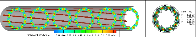
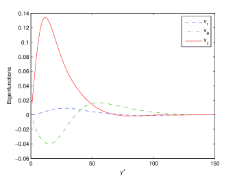
Figure 11a: Most energetic propagating wall mode (1,5,1). Coherent vorticity (left) and a cross-section of coherent vorticity with Reynolds stress superimposed (right).

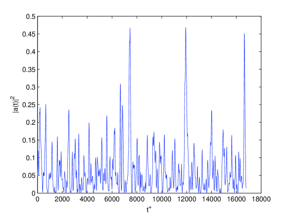
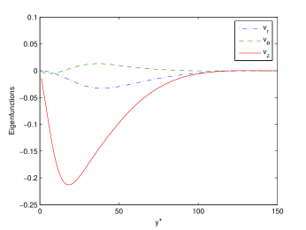
Figure 11b: Real component of (1,5,1).	Figure 11c: Time history amplitude of (1,5,1).
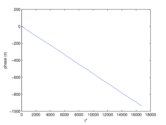
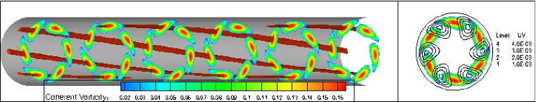
Figure 11d: Imaginary component of (1,5,1).	Figure 11e: Time history phase of (1,5,1).

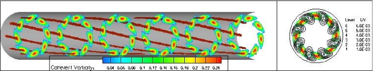
Figure 11f: Propagating wall mode (1,3,1).

Figure 11g: Propagating wall mode (2,4,1).

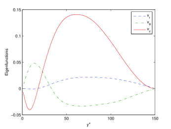
Figure 12a: Most energetic propagating lift mode (2,2,1). Coherent vorticity (left) and a cross-section of coherent vorticity with Reynolds stress superimposed (right).

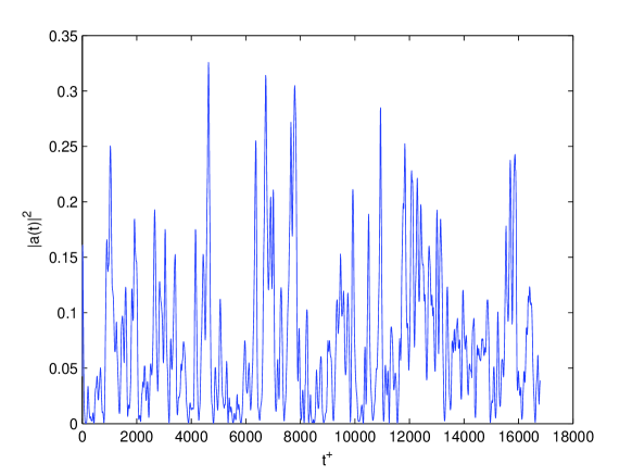
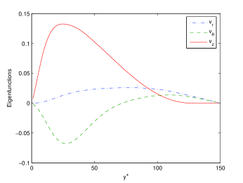
Figure 12b: Real component of (2,2,1)	Figure 12c: Time history amplitude of (2,2,1)
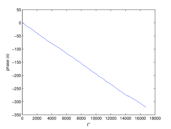
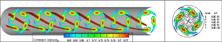
Figure 12d: Imaginary component of (2,2,1)	Figure 12e: Time history phase of (2,2,1)

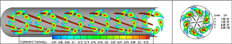
Figure 12f: Propagating lift mode (3,2,1).

Figure 12g: Propagating lift mode (3,3,1).

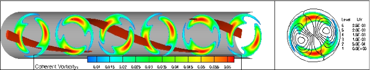
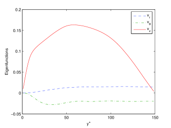
Figure 13a: Most energetic propagating asymmetric mode (1,1,1). Coherent vorticity (left) and a cross-section of coherent vorticity with Reynolds stress superimposed (right).

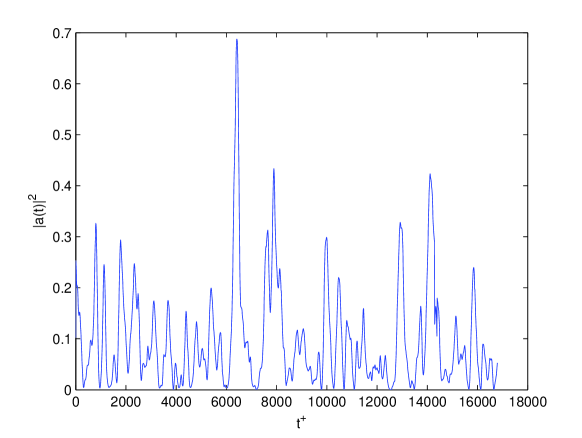
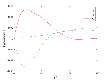
Figure 13b: Real component of (1,1,1).	Figure 13c: Time history amplitude of (1,1,1).
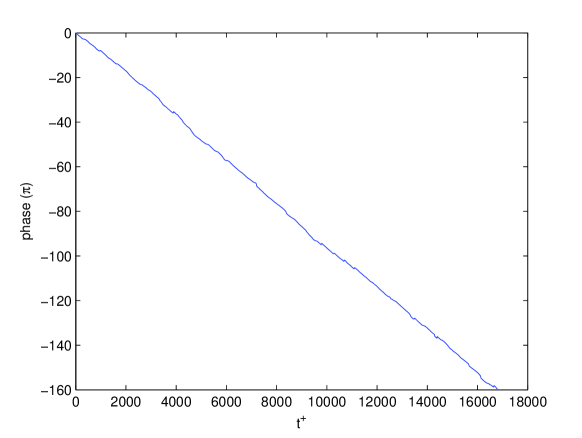
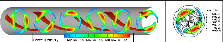
Figure 13d: Imaginary component of (1,1,1).	Figure 13e: Time history phase of (1,1,1).

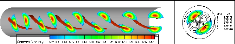
Figure 13f: Propagating asymmetric mode (2,1,1).

Figure 13g: Propagating asymmetric mode (3,1,1).

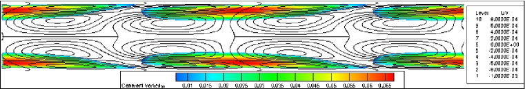
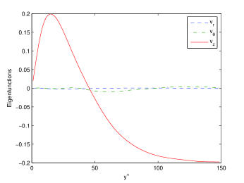
Figure 14a: Most energetic propagating ring mode (1,0,1) cross-section. Coherent vorticity with Reynolds stress superimposed.

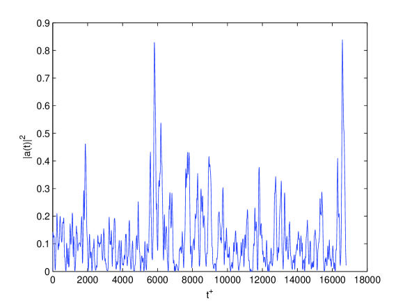
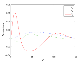
Figure 14b: Real component of (1,0,1).	Figure 14c: Time history amplitude of (1,0,1).
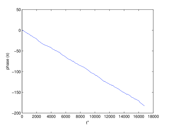
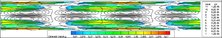
Figure 14d: Imaginary component of (1,0,1).	Figure 14e: Time history phase of (1,0,1).

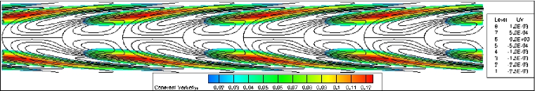
Figure 14f: Propagating ring mode (1,0,2).

Figure 14g: Propagating ring mode (2,0,1).

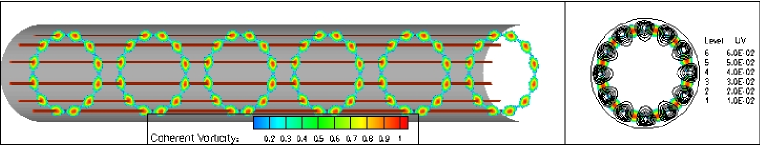
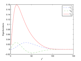
Figure 15a: Most energetic non propagating roll mode (0,6,1). Coherent vorticity (left) and a cross-section of coherent vorticity with Reynolds stress superimposed (right).

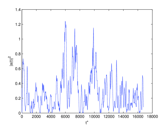
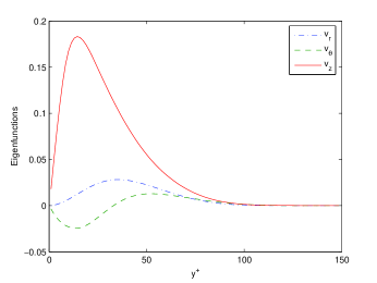
Figure 15b: Real component of (0,6,1).	Figure 15c: Time history amplitude of (0,6,1).
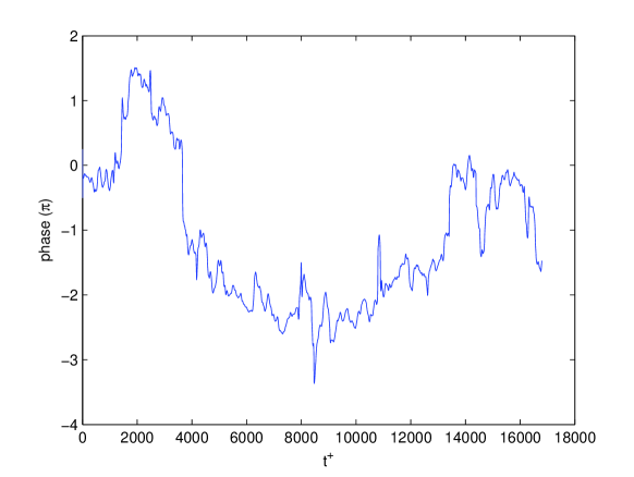
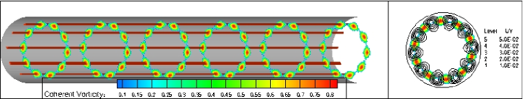
Figure 15d: Imaginary component of (0,6,1).	Figure 15e: Time history phase of (0,6,1).

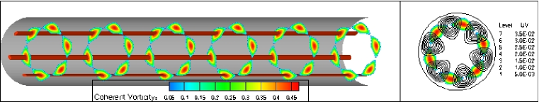
Figure 15f: Non propagating roll mode (0,5,1).

Figure 15g: Non propagating roll mode (0,3,1).

Figure 16a: Real component of (0,0,1).	Figure 16b: Time history amplitude of (0,0,1).
Figure 16c: Real component of (0,0,2).	Figure 16d: Time history phase of (0,0,1).

The energy spectra of the propagating mode subclasses are shown in Figure 17. This shows that the tail wavenumber end of the inertial range is populated primarily by the lift modes and the low end of the spectra is populated predominantly by the wall modes. The physical meaning of this is that the energy starts at the wall with large scale structures and is lifted away from the wall into the outer region in small scale structures, represented by the lifting modes.

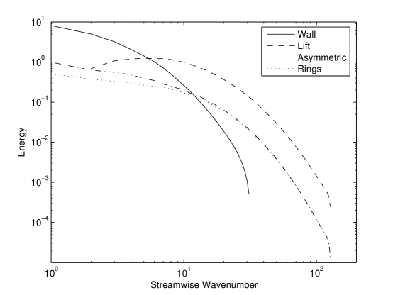
Figure 17: Energy spectra for the propagating mode subclasses, wall (solid), lift (dashed), asymmetric (dash-dot), and rings (dots). The wall modes correspond to the low wavenumber energy and the lift modes represent the high wavenumber spectra commonly known as the inertial range.

The effect of higher radial quantum number $q>1$ is more zero crossings of the velocities in the radial direction. The effect on the location of coherent vorticity and the number of vortex cores scales with the radial quantum number $q$, making the subclasses invariant with $q$. The wall and lift modes retain their characteristics, in that even with more vortices, they remain close to the wall for the wall mode and close to the centreline for the lift modes, shown in Figures 19b through 19b.

Figure 18a: (6,2,3) lift mode, contours of coherent vorticity.	Figure 18b: (6,2,5) lift mode, contours of coherent vorticity.
Figure 19a: (2,6,3) wall mode, contours of coherent vorticity.	Figure 19b: (2,6,5) wall mode, contours of coherent vorticity.

4 Discussion

Although the Karhunen-Loève method yields a preferred or natural basis for turbulence, one must be careful in the conclusions drawn from the results, as any structure or feature can be reconstructed from any given orthogonal basis. The strength of this method is that it is the most optimal basis, and by focusing on the most energetic modes a low order dynamical representation of the flow is realised. This low order dynamical system reveals three important results, and paints a picture of the energy dynamics in turbulent pipe flow.

The first result is the constant phase speed of the propagating modes. This was also found in studies of turbulent channel flow, as the structures represented by the basis advect with a constant group velocity, the same average velocity of burst events [13, 14, 15]. The normal speed locus of the propagating waves is shown in Figure 20 for the propagating modes found in the top 50 most energetic modes. For this, the phase speed $\omega/\|\mathbf{k}\|$ is plotted in the direction $\mathbf{k}/\|\mathbf{k}\|$. The locus is nearly circular, which is evidence that these structures propagate as a wave packet or envelope that travels with speed of $8.41U_{\tau}$, the point at which the circle intersects the x-axis in Figure 20, which corresponds to the mean velocity in the buffer region at $y^{+}=9.6$.

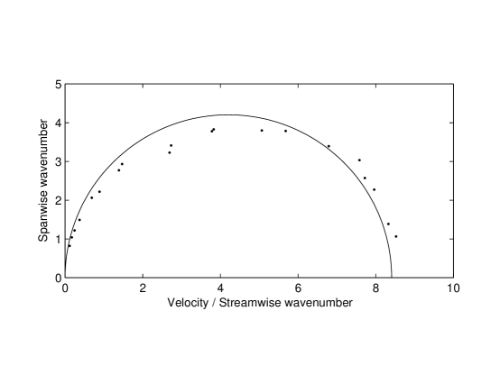
Figure 20: Normal speed locus of top 25 most energetic propagating eigenfunctions, normalised with shear velocity $u_{\tau}$. The circle is a least-squares fit to the data and represents that the wave packets are acting together as a group with speed of 8.41 $U_{\tau}$, the point where the circle intersects the y-axis.

The second interesting result is that none of the modes with azimuthal wave number $n=1$ exhibit any travelling waves near the wall, and are without exception a streamwise or inclined streamwise vortex in the outer region. The reason is that the $n=1$ mode does not allow for a near-wall travelling wave as found by Kerswell [34], and as such, the basis expansions for these modes have only near-centreline structures.

The third result of note is that the different KL structures, as observed from our results, can be seen qualitatively as an expansion that represents the horseshoe (hairpin) vortex representation of turbulent structures. This horseshoe structure is supported by a large number of researchers in the turbulence community as the self-sustaining mechanism for turbulence [1]. In the representative horseshoe structure (see, for example, the figure by Theodorsen [35]), the structures found in the KL can be seen. The wall modes represent the leg structure and its perturbation near the wall. The lift modes represent the structure lifting off the wall. The asymmetric modes represent the secondary and tertiary horseshoes that are formed. The turn modes represent the spanwise head of the horseshoe. As mentioned before, since the KL decomposition forms a basis, any flow can be recreated from these eigenmodes, so this result is reported as an interesting qualitative result, and as an understanding that the propagating modes are the structures of interest in turbulence.

The final dynamical picture of the KL modes in summarising the work done by Kerswell [34], Webber et al. [20, 21], Sirovich et al. [14], and this current work is as follows. Webber et al. found that the energy enters the flow from the pressure gradient to the shear modes. The shear modes, interacting with the roll modes present in fully developed turbulence transfers the energy from the shear modes to the roll modes. Shown in this study, and theoretically by Kerswell, the roll modes decay much more slowly than the propagating modes. Because of this slow decay, these streamwise rolls provide an energy storage role in the turbulence, similar to a capacitance. This allows enough time for the roll to interact with the propagating wave packet shown by Sirovich et al. Because this interaction requires a finite time to occur, the energy storage and slow decaying nature of the streamwise rolls play an integral role in the self-sustaining nature of turbulence. It is also surmised that the travelling modes found by Kerswell and other researchers are represented in the KL formulation as the most unstable wave packet of KL modes. Following again the work of Webber et al. and applying the classifications found in this study, the majority of the energy from the roll modes are transferred to the wall modes. The wall modes then interact with themselves through an asymmetric mode catalyst, and with the lift modes through a ring mode catalyst. Physically, this gives a picture of wall turbulence energy being transferred near the wall and then lifted up to the outer layer. This interaction between the wall and the lift modes is what populates the inertial range shown in figure 17. The energy is ultimately dissipated by viscosity, faster for the higher wavenumber modes.

5 Conclusions

We have presented the use of the Karhunen-Loève expansion method with the results of a globally high-order direct numerical simulation of turbulent pipe flow. The results reveal the structure of the turbulent pipe flow as propagating (80.58% total energy) and non propagating modes (19.42% total energy). The propagating modes are characterised by a constant phase speed and have four distinct classes: wall, lift, asymmetric, and ring modes. These propagating modes form a travelling wave envelope, forming a circular, normal-speed locus, with advection speed of $8.41U_{\tau}$ corresponding to the mean velocity in the buffer region near $y^{+}=9.6$. The non propagating modes have two subclasses: streamwise roll and shear modes. These represent the energy storage and mean fluctuations of the turbulent flow, respectively. The energy is transferred from the streamwise rolls to the wall modes first, and then later to the lift modes, physically representing the energy transfer from the wall to the outer region. This eigenfunction expansion, using both their structure and their time-dependent coefficients, provides a framework for understanding the dynamics of turbulent pipe flow, and will provide a basis for further analysis and comparison leading to understanding the mechanism of drag reduction by spanwise wall oscillation [36] and the mechanism of relaminarization [37].

References

- [1] R. Panton, 2001. Overview of the Self-sustaining Mechanisms of Wall Turbulence. Prog. Aero. Sci., 37, 343–383.
- [2] Patel, V.C., and Head, M.S., 1969. Some observations on skin friction and velocity profiles in fully developed pipe and channel flows. J. Fluid Mech.,, 38, 181–201.
- [3] Durst, F., Jovanovic, J., and Sender, J., 1995. LDA measurements in the near-wall region of a turbulent pipe flow. J. Fluid Mech., 295, 305–335.
- [4] Orszag, S.A., and Patera, A.T., 1983. Secondary instability in wall-bounded shear flows. J. Fluid Mech., 128, 347–385.
- [5] O’Sullivan, P.L, and Breuer, K.S., 1994. Transient growth in circular pipe flow, 1: Linear disturbances. Phys. Fluids, 6, 11, 3643–3651.
- [6] Shan, H., Ma, B., Zhang, Z., and Nieuwstadt, F.T.M., 1999. Direct numerical simulation of a puff and a slug in transitional cylindrical pipe flow. J. Fluid Mech., 387, 39–60.
- [7] Loulou, P., Moser, R.D., Mansour, N.N., and Cantwell, B.J., 1997. Direct Numerical Simulation of Incompressible Pipe Flow Using a B-Spline Spectral Method. NASA Technical Memorandum-110436.
- [8] Eggels, J.G.M., Unger, F., Weiss, W.H., Westerweel, J., Adrian, R.J., Friedrich, R., and Nieuwstadt, F.T.M., 1994. Fully developed turbulent pipe flow: A comparison between direct numerical simulation and experiment. J. Fluid Mech., 268, 175–209.
- [9] Verzicco, R., and Orlandi, P., 1996. A finite-difference scheme for three-dimensional incompressible flows in cylindrical coordinates J. Comp. Phys, 123, 402–414.
- [10] Fukagata, K., and Kasagi, N., 2002. Highly energy-conservative finite difference method for the cylindrical coordinate system. J. Comp Phys., 181, 478–498.
- [11] Lumley, J.L., 1967. The structure of inhomogeneous turbulent flows. Atmospheric Turbulence and Radio Wave Propagation, Yaglom, A.M. and Tatarski, V.I. (eds), (Nauka, Moscow) 166–178.
- [12] Lumley, J.L. 1970. Stochastic Tools in Turbulence. Academic Press, (New York).
- [13] Ball, K.S., Sirovich, L., and Keefe, L.R., 1991. Dynamical eigenfunction decomposition of turbulent channel flow. Int. J. Numer. Meth. Fluids, 12, 585–604.
- [14] Sirovich, L., Ball, K.S., and Keefe, L.R., 1990. Plane waves and structures in turbulent channel flow. Phys. Fluids A, 12, 2217–2226.
- [15] Sirovich, L., Ball, K.S., and Handler, R.A,,1991. Propagating structures in wall-bounded turbulent flows. Theoret. Comput. Fluid Dynamics, 2, 307–317.
- [16] Aubry, N, Holmes, P., Lumley, J.L., Stone, E., 1988. The dynamics of coherent structures in the wall region of a turbulent boundary layer. J. Fluid Mech., 192, 115–173.
- [17] Zhou,X., and Sirovich, L., 1992. Coherence and chaos in a model of the turbulent boundary layer. Phys. Fluids A, 4, 2855–2874.
- [18] Sirovich L., and Zhou, X., 1994. Dynamical model of wall bounded turbulence. Phys. Rev. Lett., 72, 340–343.
- [19] Smith, T.R., J. Moehlis, and P. Holmes, 2005. Low-dimensional models for turbulent pipe Coutette flow in a minimal flow unit. J. Fluid. Mech., 538, 71–110.
- [20] Webber, G.A., Handler, R.A., and Sirovich L., 1997. The Karhunen-Loève decomposition of minimal channel flow. Phys. Fluids, 9, 1054–1066.
- [21] Webber, G.A., Handler, R.A, and Sirovich, L., 2002. Energy dynamics in a turbulent channel flow using the Karhunen-Loève approach. Int. J. Numer. Meth. Fluids, 40, 1381–1400.
- [22] Boyd, J.P., 2000. Chebyshev and Fourier Spectral Methods. DOVER Publications, Mineola, New York.
- [23] Fischer, P.F., Ho, L.W., Karniadakis, G.E, Ronouist, E.M., and Patera, A.T., 1988. Recent advances in parallel spectral element simulation of unsteady incompressible flows. Comput. & Struct., 30, 217–231.
- [24] Tufo, H.M., and Fischer, P.F., 1999. Terascale spectral element algorithms and implementations, Proceedings of the ACM/IEEE SC99 Conference on High Performance Networking and Computing, IEEE Computer Soc., Gordon Bell Prize paper.
- [25] Lottes, J.W. and Fischer, P.F., 2004. Hybrid multigrid/Schwarz algorithms for the spectral element method. J. Sci. Comp., 24, 45–78.
- [26] Paul, M.R., Chiam, K.H., and Cross, M.C., 2004. Rayleigh-Benard convection in large-aspect-ratio domains. Phys. Rev. Lett., 93, 064503.
- [27] Gullbrand, J., 2000. An evaluation of a conservative fourth order DNS code in turbulent channel flow. Center for Turbulence Research, Anual Research Briefs.
- [28] Jiménez, J. 1998. The largest scales of turbulent wall flows Center for Turbulence Research, Annual Research Briefs.
- [29] Sirovich, L., 1987. Turbulence and the dynamics of coherent structures, Part I: Coherent Structures. Q. Appl. Math., XLV 3, 561–571.
- [30] Sirovich, L., 1987. Turbulence and the dynamics of coherent structures, Part II: Symmetries and transformations. Q. Appl. Math., XLV 3, 573–582.
- [31] Sirovich, L., 1987. Turbulence and the dynamics of coherent structures, Part III: Dynamics and scaling. Q. Appl. Math., XLV 3, 583–590.
- [32] Sirovich, L., 1989. Chaotic dynamics of coherent structures. Phys. D, 37, 126–143.
- [33] Chong, M.S., Perry, A. E., and Cantwell, B. J., 1990. A general classification of three-dimensional flow fields Phys. Fluids A, 2, 765–777.
- [34] Kerswell, R.R., 2005. Recent progress in understanding the transition to turbulence in a pipe. Nonlinearity, 18, R17–R44.
- [35] Theodorsen, T. 1952. Mechanism of turbulence. Proceedings of the Second Midwestern Conference on Fluid Mechanics, Ohio State University, 1–18.
- [36] Duggleby, A., Ball, K.S., and Paul, M.R., 2006. Dynamics of propagating turbulent pipe flow structures. Part I: Effect of drag reduction by spanwise wall oscillation. Phys. Fluids, in review.
- [37] Duggleby, A., Ball, K.S., and Paul, M.R., 2006. Dynamics of propagating turbulent pipe flow structures. Part II: Relaminarization Phys. Fluids, in review.