Hitting Time Distributions in Financial Markets

Abstract

We analyze the hitting time distributions of stock price returns in different time windows, characterized by different levels of noise present in the market. The study has been performed on two sets of data from US markets. The first one is composed by daily price of 1071 stocks trade for the 12-year period 1987-1998, the second one is composed by high frequency data for 100 stocks for the 4-year period 1995-1998. We compare the probability distribution obtained by our empirical analysis with those obtained from different models for stock market evolution. Specifically by focusing on the statistical properties of the hitting times to reach a barrier or a given threshold, we compare the probability density function (PDF) of three models, namely the geometric Brownian motion, the GARCH model and the Heston model with that obtained from real market data. We will present also some results of a generalized Heston model.

I Introduction

The interest of physicists in intedisciplinary researches has been largely increased in recent years and one of the developing field in this context is econophysics. It applies and proposes ideas, methods and models in statistical physics and physics of complex systems to analyze data coming from economical phenomena Farmer . Several statistical properties verified in financial quantities such as relative price changes or returns and their standard deviation, have enabled the establishment of new models which characterize systems ever better Mantegna-Stanley . Moreover the formalism used by physicists to analyze and to model complex systems constitutes a specific contribution that physics gives to many other fields. Complex systems in fact provide a very good paradigm for all those systems, physical and non-physical ones, whose dynamics is driven by the nonlinear interaction of many agents in the presence of ”natural” randomness Anderson . The simplest universal feature of financial time series, discovered by Bachelier Bachelier , is the linear growth of the variance of the return fluctuations with time scale, by considering the relative price changes uncorrelated. The availability of high frequency data and deeper statistical analyses invalidated this first approximated model Mantegna-Stanley , which is not adequate to catch also other important statistical peculiarities of financial markets, namely: (i) the non-Gaussian distribution of returns, (ii) the intermittent and correlated nature of return amplitudes, and (iii) the multifractal scaling Borl-Bouc , that is the anomalous scaling of higher moments of price changes with time.

In this paper we focus our attention on the statistical properties of the first hitting time (FHT), which refers to the time to achieve a given fixed return or a given threshold for prices. Theoretical and empirical investigations have been done recently on the mean exit time (MET) Mas and on the waiting times Scalas of financial time series. We use also the term ”escape time” to include the analysis of times between different dynamical regimes in financial markets done in a generalized Heston model spagnolo-pre06 . Markets indeed present days of normal activity and extreme days where high price variations are observed, like crash days. To describe these events, a nonlinear Langevin market model has been proposed in Refs. BouchaudCont , where different regimes are modelled by means of an effective metastable potential for price returns with a potential barrier. We will discuss three different market models evidencing their limits and features, by comparing the PDF of hitting times of these models with those obtained from real financial time series. Moreover we will present some recent results obtained using a generalized Heston model.

II Models for stock market evolution

II.1 The geometric random walk

The most widespread and simple market model is that proposed by Black and Scholes to address quantitatively the problem of option pricing Black . The model assumes that the price obeys the following multiplicative stochastic differential equation

$$d\,p(t)=\mu\cdot p(t)\cdot dt+\sigma\cdot p(t)\cdot dW(t)$$ (1)

where $\mu$ and $\sigma$ are the expected average growth for the price and the expected noise intensity (the volatility) in the market dynamics respectively. $dp/p$ is usually called price return. The model is a geometric random walk with drift $\mu$ and diffusion $\sigma$. By applying the Ito’s lemma we obtain for the logarithm of the price

$$d\,lnp(t)=(\mu-\frac{\sigma^{2}}{2})\cdot dt+\sigma\cdot dW(t)\;.$$ (2)

This model catches one of the more important stylized facts of financial markets, that is the short range correlation for price returns. This characteristic is necessary in order to warrant market efficiency. Short range correlation indeed yields unpredictability in the price time series and makes it difficult to set up arbitrage strategies.

The statistical properties of escape times $\tau$ for this process are well known, and the PDF of escape time $\tau$, $F(\tau,p_{0})$, was obtained analytically Wilmott . If the starting value of the price is $p_{0}$ at time $t=0$, the distribution of the time $\tau$ to reach a barrier at position $h$ is given by the so called inverse Gaussian

$$F(\tau,p_{0})=\frac{h-p_{0}}{\sqrt{2\pi\sigma^{2}\tau^{3}}}\cdot exp\left[-\frac{(h-p_{0}-\mu\tau)^{2}}{2\sigma^{2}\tau}\right],$$ (3)

which is well known among finance practitioners to price exotic options like barrier options Wilmott or to evaluate the probability for a firm to reach the zero value where it will remain forever. The shape of the distribution is shown in Fig. 1 for two different cases. The asymptotic expressions of PDF show in one case a power law tail with exponent -1.5

$$F(\tau,p_{0})\mid_{\tau\rightarrow\infty}\;\;\simeq\frac{h-p_{0}}{\sqrt{2\pi\sigma^{2}}}\;\;\tau^{-3/2}\;,\;\;\;\mu=0$$ (4)

and a dominat exponential behavior in the other case

$$F(\tau,p_{0})\mid_{\tau\rightarrow\infty}\;\;\simeq\frac{h-p_{0}}{\sqrt{2\pi\sigma^{2}}}\;\;\tau^{-3/2}\;exp\left[-\frac{\mu^{2}}{2\sigma^{2}}\;\;\tau\right],\;\;\;\mu\neq 0.$$ (5)

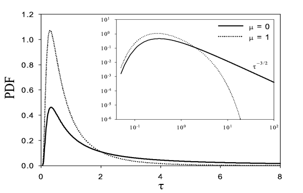
Figure 1: Inverse Gaussian distribution obtained with the parameters $\sigma=1.0$, $(h-p_{0})=1.0$, for $\mu=0$ (solid line) and $\mu=1$ (dotted line). Inset: log-log plot of the same PDF.

The distribution of hitting times for price returns instead is very simple. In the geometric Brownian motion the returns are independent, so the probability to observe a value after a certain barrier is given by the probability that the ”particle” doesn’t escape after $n-1$ time steps, multiplied by the escape probability at the $n^{th}$ step

$$F_{r}(\tau)=(1-p)\cdot p^{n-1}=((1-p)\cdot exp\left[(n-1)\ln p\right],\;\;\;n=\frac{\tau}{\Delta t}$$ (6)

where $p$ is the probability to observe a return inside the region defined by the barrier, $\Delta t$ is the observation time step and $\tau$ is the escape time. So the probability is exponential in time. The geometric Brownian motion is not adequate to describe financial markets behavior, because the volatility is considered as a constant parameter and the PDF of the price is a log-normal distribution.

II.2 The GARCH and the Heston models

Price returns have indeed properties that cannot be reproduced by the previous simple model: (i) price return distribution has fat tails; (ii) price returns have short range correlation but the volatility is a stochastic process with long range correlation Man-Sta95 . The degree of variability in time of the volatility indeed depends not only on the Fundamentals of the firm but also on the market conditions. Volatility is usually higher during crisis periods and has also an almost deterministic intra-day pattern during the trading day, being higher near market opening and closure. So the volatility can be considered as a stochastic process itself and it is characterized by long range memory and clustering. More realistic models to reproduce the dynamics of the volatility have been developed. Here we will present two of them: the GARCH and the Heston models.

The GARCH(p,q) process (generalized autoregressive conditional heteroskedasticity), which is essentially a random multiplicative process, is the generalization of the ARCH process and combines linearly the actual return with $p$ previous values of the variance and $q$ previous values of the square return Garch . The process is described by the equations

$$\sigma^{2}_{t}=\alpha_{0}+\alpha_{1}x^{2}_{t-1}+\dots+\alpha^{2}_{q}x^{2}_{t-q}+\beta_{1}\sigma^{2}_{t-1}+\dots+\beta_{p}\sigma^{2}_{t-p},\;\;\;\;\;\;\;x_{t}=\eta_{t}\cdot\sigma_{t},$$ (7)

where $\alpha_{i}$ and $\beta_{i}$ are parameters that can be estimated by means of a best fit of real market data, $x_{t}$ is a stochastic process representing price returns and is characterized by a standard deviation $\sigma_{t}$. The GARCH process has a non-constant conditional variance but the variance observed on long time period, called unconditional variance, is instead constant and can be calculated as a function of the model parameters. It has been demonstrated that $x_{t}^{2}$ of GARCH(1,1) is a Markovian process with exponential autocorrelation, while the autocovariance of GARCH(p,q) model is a linear combination of exponential functions Mantegna-Stanley ; Garch . We will consider the simpler GARCH(1,1) model

$$\sigma^{2}_{t}=\alpha_{0}+(\alpha_{1}\eta_{t-1}^{2}+\beta_{1})\sigma^{2}_{t-1},\;\;\;\;\;x_{t}=\eta_{t}\cdot\sigma_{t}\;.$$ (8)

The autocorrelation function of the process $x_{t}$ is proportional to a delta function, while the process $x_{t}^{2}$ has a correlation characteristic time equal to $\tau=\mid ln(\alpha_{1}+\beta_{1})\mid^{-1}$ and the unconditional variance equal to $\sigma^{2}=\alpha_{0}/(1-\alpha_{1}-\beta_{1})$. So it is possible to fit the empirical values of these two quantities by adjusting few parameters. Specifically $\alpha_{1}$ and $\beta_{1}$ regulate the characteristic time scale in the correlation, while $\alpha_{0}$ can be adjusted independently to fit the observed unconditional variance.

In the Heston model Heston the dynamics is described by a geometric Brownian motion coupled to a second stochastic process for the variable $v=\sigma^{2}$. The model equations are

$$d\,lnp(t) = (\mu-\frac{v(t)}{2})\cdot dt+\sqrt{v(t)}\cdot dW(t),$$ (9)

$$dv(t) = a(b-v(t))\cdot dt+c\sqrt{v(t)}\cdot dZ(t),$$

where $W(t)$ and $Z(t)$ are uncorrelated Wiener processes with the usual statistical properties $<dW_{i}>\;=0,\;<dW_{i}(t)dW_{j}(t^{\prime})>\;=\delta(t-t^{\prime})~{}\delta_{i,j}$, but can be also correlated Silva . The process for $v$ is called Cox-Ingersoll-Ross CIR and has the following features: (i) the deterministic solution tends exponentially to the level $b$ at a rate $a$ (mean reverting process); (ii) the autocorrelation is exponential with time scale $\tau=a^{-1}$. Here $c$ is the amplitude of volatility fluctuations often called the volatility of volatility. Once again we have a model with short range correlation that mimics the effective long range correlation of the markets using large values of $\tau$. The process is multiplicative and values of $v$ can be amplified in few steps producing bursts of volatility. If the characteristic time is large enough, many steps will be required to revert the process to the mean level $b$. So the longer the memory is, the longer the burst will survive. For little correlation times the process fluctuates uniformly around the mean level $b$, whereas for large correlation times $v$ presents an intermittent behavior with alternating activity of burst and calm periods. The model has been recently investigated by econophysicists  Silva and solved analytically Yako .

The two models presented so far are a more realistic representation of financial market than the simple geometric Brownian motion, even if they do not reproduce quantitatively the form of the long time correlation observed for the volatility. We use a set of 1071 daily stock price returns for the 12-year period 1987-1998, and we compare the results obtained by simulation of the GARCH and Heston models with those obtained from real market data. The parameters in the models were chosen by means of a best fit, in order to reproduce the correlation properties and the variance appropriate for real market. Specifically for the GARCH model we used values $\alpha_{1}=0.07906$ and $\beta_{1}=0.90501$ obtained elsewhere Akgiray to fit the correlation time of daily market data, and $\alpha_{0}=7.7\cdot 10^{-6}$ in order to fit the average standard deviation of our data using the formula for unconditional variance presented in the previous section. For the Heston model we used $a=4.5\cdot 10^{-2}$, $b=8.62\cdot 10^{-5}$ and $\mu=5.67\cdot 10^{-4}$, obtained in a recent work Yako , suitable for daily returns and $c=10.3\cdot 10^{-3}$, as before, to fit the average standard deviation of our data set. Using these parameters we obtain distribution for price returns that are in reasonable agreement with real market data, as shown in Fig. 2.

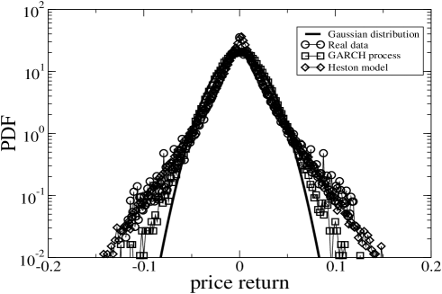
Figure 2: Probability density function of stock price returns for: real market data (circle), GARCH model (square) and Heston model (diamond). The black solid line is a Gaussian distribution having the same standard deviation of real data.

The two models approximate the return distributions of real data better than the Gaussian curve. In particular the Heston model gives the best agreement. The chosen parameter set therefore is good enough to fit the dynamics of our data.

In order to investigate the statistical properties of escape times $\tau$ we choose two thresholds to define the start and the end for the random walk. Specifically we calculate the standard deviation $\sigma_{i}$, with $i=1,\dots,1071$ for each stock over the whole 12-year period. Then we set the initial threshold to the value $0.1\cdot\sigma_{i}$ and as final threshold the value $-2\cdot\sigma_{i}$. The thresholds are different for each stock, the final threshold is considered as an absorbing barrier. The resulting experimental distribution reported in Fig. 3 has an exponential tail but it deviates from the exponential behavior in the region of low escape times. Specifically low escape times have probability higher than the exponential. We recall that for the geometric Brownian motion model this distribution should be exponential over the entire $\tau$ axis. So the first conclusion we can draw from our analysis is that the basic geometric Brownian motion is not adequate to explain the distribution of $\tau$.

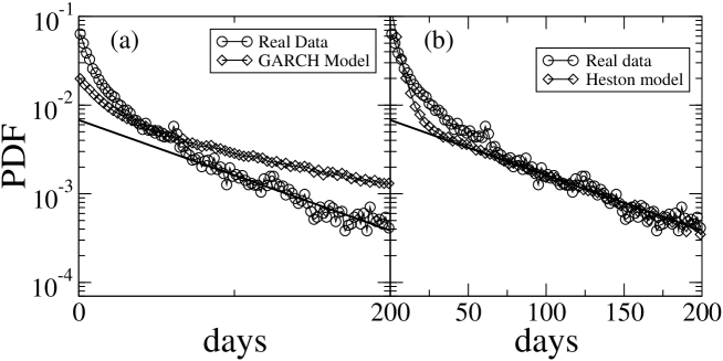
Figure 3: PDF of escape times of price returns for the (a) GARCH and (b) Heston models (diamond) compared with the distribution obtained from real market data (circle). The process starts at $(-0.1\sigma)=-0.0022$, the barrier is located at $(-2.0\sigma)$. The straight line is an exponential fit of the distribution tail.

In order to reproduce more closely the situation present in real market we choose $\sigma_{start}$ only once, specifically we place the random walker in the initial starting position and we set the initial volatility value. When the random walker hits the barrier, we register the time and we place the walker again in the initial position, using the volatility of the barrier hitting time. So the random walker can experience different initial volatility values as in real markets. The results are reported in the two panels of Fig. 3 for both the GARCH and the Heston models, and we see that these models provide a better agreement with real data than the geometric Brownian motion. Moreover for the GARCH model the agreement is only qualitative, whereas the Heston model is able to fit the empirical distribution quantitatively.

II.3 The modified Heston model

Here we consider a generalization of the Heston model, by considering a cubic nonlinearity. This generalization represents a fictitious ”Brownian particle” moving in an effective potential with a metastable state, in order to model those systems with two different dynamical regimes like financial markets in normal activity and extreme days BouchaudCont . The equations of the new model are

$$dx(t) = -\left(\frac{\partial U}{\partial x}+\frac{v(t)}{2}\right)~{}dt+\sqrt{v(t)}~{}dW_{1}(t)$$ (10)

$$dv(t) = a(b-v(t))~{}dt+c\sqrt{v(t)}~{}dW_{2}(t),$$ (11)

where $U(x)=2x^{3}+3x^{2}$ is the effective cubic potential with a metastable state at $x_{me}=0$, a maximum at $x_{M}=-1$, and a cross point between the potential and the $x$ axes at $x_{I}=-1.5$. In systems with a metastable state like this, the noise can originate the noise enhanced stability (NES) phenomenon, an interesting effect that increases, instead of decreasing, the stability by enhancing the lifetime of the metastable state NES ; Nes-theory . The mean escape time $\tau$ for a Brownian particle moving throughout a barrier $\Delta U$, with a noise intensity $v$, is given by the the well known exponential Kramers law $\tau=exp\left[\Delta U/v\right]$, where $\tau$ is a monotonically decreasing function of the noise intensity $v$. This is true only if the random walk starts from initial positions inside the potential well. When the starting position is chosen in the instability region $x_{o}<x_{M}$, $\tau$ exhibits an enhancement behavior, with respect to the deterministic escape time, as a function of $v$. This is the NES effect and it can be explained considering the barrier ”seen” by the Brownian particle starting at the initial position $x_{0}$, that is $\Delta U_{in}=U(x_{max})-U(x_{0})$. In fact $\Delta U_{in}$ is smaller than $\Delta U$ as long as the starting position $x_{0}$ lies in the interval $I=[x_{I},x_{M}]$. Therefore for a Brownian particle starting from an unstable initial position, from a probabilistic point of view, it is easier to enter into the well than to escape from, once the particle is entered. So a small amount of noise can increase the lifetime of the metastable state. For a detailed discussion on this point and different dynamical regimes see Refs. Nes-theory . When the noise intensity $v$ is much greater than $\Delta U$, the Kramers behavior is recovered.

Here, by considering the modified Heston model, characterized by a stochastic volatility and a nonlinear Langevin equation for the returns, we study the mean escape time as a function of the model parameters $a$, $b$ and $c$. In particular we investigate whether it is possible to observe some kind of nonmonotonic behavior such that observed for $\tau~{}vs.~{}v$ in the NES effect with constant volatility $v$. We call the enhancement of the mean escape time (MET) $\tau$, with a nonmonotonic behavior as a function of the model parameters, NES effect in the broad sense. Our modified Heston model has two limit regimes, corresponding to the cases $a=0$, with only the noise term in the equation for the volatility $v(t)$, and $c=0$ with only the reverting term in the same equation. This last case corresponds to the usual parametric constant volatility regime. In fact, apart from an exponential transient, the volatility reaches the asymptotic value $b$, and the NES effect is observable as a function of $b$. To this purpose we perform simulations by integrating numerically the equations (10) and (11) using a time step $\Delta t=0.01$. The simulations were performed placing the walker in the initial positions $x_{0}$ located in the unstable region $[x_{I},x_{M}]$ and using an absorbing barrier at $x=-6.0$. When the walker hits the barrier, the escape time is registered and another simulation is started, placing the walker at the same starting position $x_{0}$, but using the volatility value of the barrier hitting time.

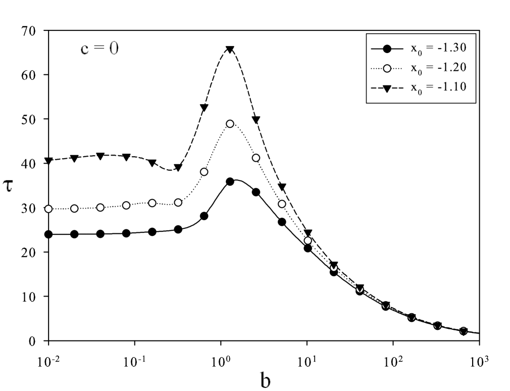
Figure 4: Mean escape time $\tau$ for $3$ different unstable starting positions, when only the reverting term is present: $a=10^{-2}$, $c=0$).

The mean escape time as a function of $b$ is plotted in Fig. 4 for the $3$ different starting unstable positions and for $c=0$. The curves are averaged over $10^{5}$ escape events. The nonmonotonic behavior is present. After the maximum, when the values of $b$ are much greater than the potential barrier height, the Kramers behavior is recovered. The nonmonotonic behavior is more evident for starting positions near the maximum of the potential. For $a=0$ the system is too noisy and the NES effect is not observable as a function of parameter $c$. The presence of the reverting term therefore affects the behavior of $\tau$ in the domain of the noise term of the volatility and it regulates the transition from nonmonotonic to monotonic regimes of MET. The results of our simulations show that the NES effect can be observed as a function of the volatility reverting level $b$, the effect being modulated by the parameter $(ab)/c$. The phenomenon disappears if the noise term is predominant in comparison with the reverting term. Moreover the effect is no more observable if the parameter $c$ pushes the system towards a too noisy region. When the noise term is coupled to the reverting term, we observe the NES effect on the variable $c$. The effect disappears if $b$ is so high as to saturate the system.

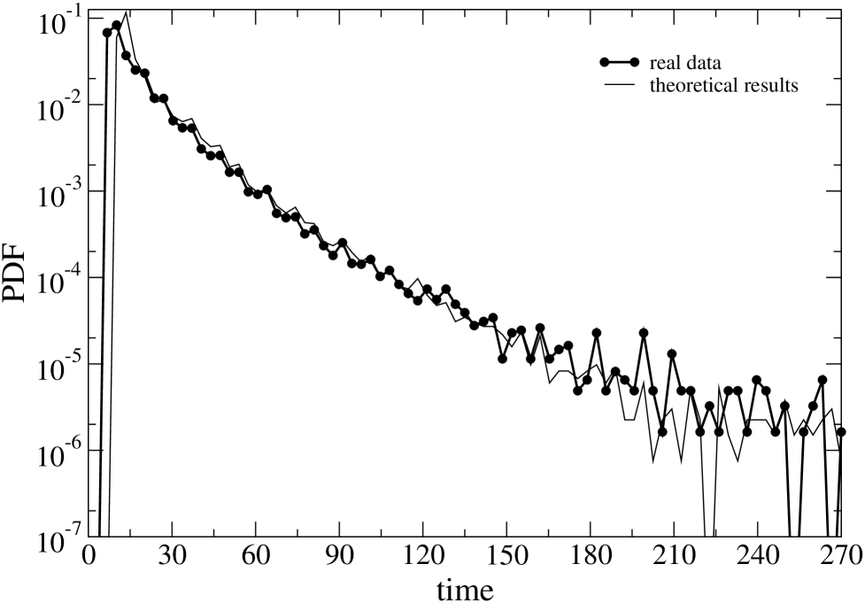
Figure 5: Probability density function of the escape time of the returns from simulation (solid line), and from real data (black circle).

We compare now the theoretical PDF for the escape time of the returns with that obtained from the same real market data used in the previous section. We define two thresholds, $\Delta x_{i}=0.1\sigma_{\Delta x}$ and $\Delta x_{f}=1.0\sigma_{\Delta x}$, which represent respectively start point and end point for calculating $\tau$. The standard deviation $\sigma_{\Delta x}$ of the return series is calculated over a long time period corresponding to that of real data. The initial position is $x_{0}=-1.25$ and the absorbing barrier is at $x_{abs}=-6.0$. For the CIR stochastic process $v$ we choose $v_{start}=8.62\cdot 10^{-5}$, $a=10^{-1}$, $b=4.5$ and $c=2\cdot 10^{-1}$. The agreement with real data is very good. At high escape times the statistical accuracy is worse because of few data with high values. The parameter values of the CIR process for which we obtain this good agreement are in the range in which we observe the nonmonotonic behavior of MET. This means that in this parameter region we observe a stabilizing effect of the noise in time windows of prices data for which we have a fixed variation of returns between $\Delta x_{i}$ and $\Delta x_{f}$. This encourages us to extend our analysis to large amounts of financial data and to explore other parameter regions of the model.

III Escape times for intra-day returns

In this last section we discuss the results obtained with the same analysis of the previous section, applied to a different data set at intra-day time scale. The data set contains 100 stocks in the 4-year period 1995–1998. The stocks considered are those used, in that period, in the S&P100 basket. We are dealing therefore with highly capitalized firms. The data are extracted from the Trade and Quote database. The stocks are distributed in different market sectors as illustrated in Ref. BonannoQF . For the analysis we considered the return on a time interval equal to $\delta t=1170sec$, which is approximately equal to $20$ minute and it is contained in a market day exactly $20$ times. So we have $19$ price returns per day, which amounts to $20220$ points in the whole period of $4$ years per each of the $100$ stocks. We used the value $-0.5\cdot\sigma$ as a start position and the value $-7.0\cdot\sigma$ as absorbing barrier. We can choose a so high value for the barrier because return distribution on intra-day time scale have tails fatter than daily return distribution, therefore the statistical accuracy for so high barrier value is good enough. The distribution of escape times obtained is reported in Fig. 6 in a semi-logarithmic plot. It has an exponential trend superimposed to a fluctuating component. One can recognize that the period of the fluctuation is 1 trading day, so this effect has to be ascribed to something that happens inside the daily activity. To describe better this aspect we record, for each barrier hitting event, the hour when the event occurs and we build a histogram showing the number of barrier hitting events as a function of the day time.

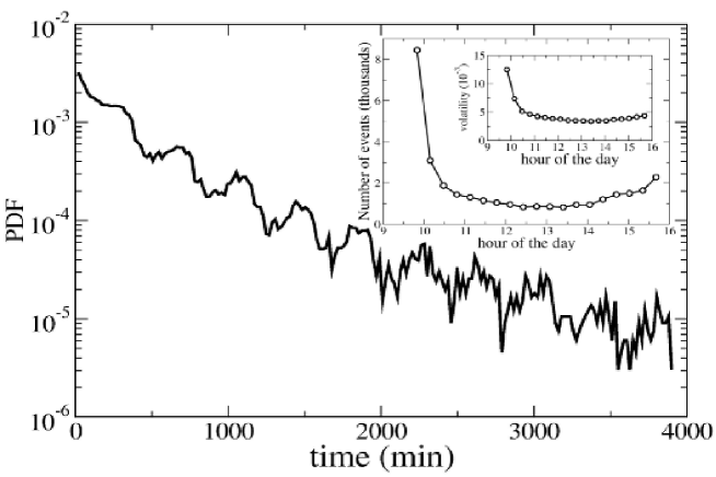
Figure 6: PDF of escape times of price returns for intra-day price returns obtained from real market data for the 100 stocks of the S&P100 basket in the 4–year period 1995–1998. The process starts at $-0.5\sigma$, the barrier is located at $-7.0\sigma$. Inset: Frequency distribution of the barrier hitting event, within a day, as a function of the hour. The internal inset shows the volatility observed in the same moment of the trading day.

This histogram (see the inset of Fig. 6) clearly shows that the barrier hitting takes place more frequently near the opening and the closure of the market. This happens because the volatility follows a well known deterministic pattern during the day, being higher near the market opening and closure, and lower in the middle of the trading day. In the same inset we report an estimation of the volatility per hour, which we calculate as the standard deviation of the return observed in that hour, in the whole period for all the 100 stocks. The figure shows that the volatility has a pattern reproducing that observed in the barrier hitting event histogram. This is in agreement with our considerations.

IV Conclusions

We studied the statistical properties of the hitting times in different models for stock market evolution. We discussed limitations and features of the basic geometric Brownian motion in comparison with more realistic market models, such as those developed with a stochastic volatility. Our results indeed show that to fit well the escape time distribution obtained from market data, it is necessary to take into account the behavior of market volatility. In the generalized Heston model the reverting rate $a$ can be used to modulate the intensity of the stabilizing effect of the noise observed (NES), by varying $b$ and $c$. In this parameter region the probability density function of the escape times of the returns fits very well that obtained from the real market data. The analysis on intra-day time scale shows another peculiarity: the intra-day volatility pattern produces periodic oscillations in the escape time distribution. This characteristic will be subject of further investigation.

References

- (1) J. Doyne Farmer, Int. J. Theoretical and Applied Finance 3, 311 (2000)
- (2) R. N. Mantegna, H. E. Stanley, An Introduction to Econophysics: Correlations and Complexity in Finance (Cambridge University Press, Cambridge, 2000); J. P. Bouchaud, M.Potters, Theory of Financial Risks and Derivative Pricing (Cambridge University Press 2004)
- (3) P. W. Anderson, K. J. Arrow, D. Pines, The Economy as An Evolving Complex System I, II (Addison Wesley Longman 1988, 1997)
- (4) L. Bachelier, Annales scientifiques de l’ecole normale supérieure III-17, 21 (1900)
- (5) Lisa Borland, Jean-Philippe Bouchaud, Jean-Francois Muzy, Gilles Zumbach, The Dynamics of Financial Markets, cond-mat/0501292 (2005)
- (6) J. Masoliver, M. Montero, J. Perell, Phys. Rev. E 71, 056130 (2005); M. Montero, J. Perell, J. Masoliver, F. Lillo, S. Miccich, R. N. Mantegna, Phys. Rev. E 72, 056101 (2005)
- (7) E. Scalas, R. Gorenflo, F. Mainardi, Physica A 284, 376 (2000); M. Raberto, E. Scalas, F. Mainardi, Physica A 314, 749 (2002)
- (8) G. Bonanno, D. Valenti, B. Spagnolo, Mean Escape Time in a System with Stochastic Volatility, Phys. Rev. E, submitted (2005)
- (9) J.-P. Bouchaud, R. Cont, Eur. Phys. J. B 6, 543 (1998); J.-P. Bouchaud, Quantitative Finance 1, 105 (2001); J.-P. Bouchaud, Physica A 313, 238 (2002)
- (10) F. Black, M. Scholes, J. Political Economy 81, 637 (1973)
- (11) P. Wilmott, Paul Wilmott on Quantitative Finance, Wiley, New York, (2000).
- (12) R. N. Mantegna, H. E. Stanley, Nature 376, 46 (1995); M. M. Dacorogna et al., An Introduction to High-Frequency Finance, Academic Press, New York, (2001)
- (13) R. F. Engle, Econometrica 50, 987 (1982); T. Bollerslev, J. Econometrics 31, 307 (1986). GARCH(p,q) models can reproduce long memory correlations because the autocovariance of the square of the process can be expressed as a sum of exponentials with different time scale , where . However with real financial data available up to now, because of limited maximum value of observation time, we cannot construct the GARCH(p,q) model with a good statistical accuracy.
- (14) S. L. Heston, Rev. Financial Studies 6, 327 (1993)
- (15) A. Christian Silva, Richard E. Prange, Victor M. Yakovenko, Physica A 344, 227 (2004)
- (16) J.P. Fouque, G. Papanicolau, K.R. Sircar, Derivatives in financial markets with stochastic volatility (Cambridge University Press, Cambridge, 2000)
- (17) A. A. Dragulescu, V. M. Yakovenko, Quantitative Finance 2, 443 (2002); S. Miccichè, G. Bonanno, F. Lillo, R.N. Mantegna, Physica A 314, 756 (2002)
- (18) V. Akgiray, J. Business 62, 55 (1989)
- (19) R. N. Mantegna, B.Spagnolo, Phys. Rev. Lett. 76, 563 (1996); A. Mielke, Phys. Rev. Lett. 84, 818 (2000)
- (20) N. V. Agudov, B. Spagnolo, Phys. Rev. E 64, 035102(R) (2001); A. Fiasconaro, B. Spagnolo, S. Boccaletti, Phys. Rev. E 72, 061110(5) (2005)
- (21) G. Bonanno, F. Lillo and R.N. Mantegna, Quantitative Finance 1, 96 (2001)