Cold collisions of OH and Rb. I: the free collision

Abstract

We have calculated elastic and state-resolved inelastic cross sections for cold and ultracold collisions in the Rb(${}^{1}S$) + OH(${}^{2}\Pi_{3/2}$) system, including fine-structure and hyperfine effects. We have developed a new set of five potential energy surfaces for Rb-OH(${}^{2}\Pi$) from high-level ab initio electronic structure calculations, which exhibit conical intersections between covalent and ion-pair states. The surfaces are transformed to a quasidiabatic representation. The collision problem is expanded in a set of channels suitable for handling the system in the presence of electric and/or magnetic fields, although we consider the zero-field limit in this work. Because of the large number of scattering channels involved, we propose and make use of suitable approximations. To account for the hyperfine structure of both collision partners in the short-range region we develop a frame-transformation procedure which includes most of the hyperfine Hamiltonian. Scattering cross sections on the order of $10^{-13}$ cm² are predicted for temperatures typical of Stark decelerators. We also conclude that spin orientation of the partners is completely disrupted during the collision. Implications for both sympathetic cooling of OH molecules in an environment of ultracold Rb atoms and experimental observability of the collisions are discussed.

I Introduction

The possibility of producing translationally ultracold molecules has recently generated great anticipation in the field of molecular dynamics. Attractive applications include the possibility of testing fundamental symmetries EDM , the potential of new phases of matter 10 ; 11a ; 11b ; 12 and the renewed quest for the control of chemical reactions through ultracold chemistry Gian ; Balak ; Bala . These endeavors are beginning to bear scientific fruit. For example, high-resolution spectroscopic measurements of translationally cold samples of OH should allow improved astrophysical tests of the variation with time of the fine-structure constant maser . The recent experimental advances Cold ; Special ; Form have made theoretical studies of the collisional behavior of cold molecules essential Krems ; Weck ; Bodo , both to interpret the data and to suggest future directions.

Several approaches have produced cold neutral molecules to date, many of which are described in Ref. Special, . The methods available can be classified into direct methods, based on cooling of preexisting molecules, and indirect methods, which create ultracold molecules from ultracold atoms. Among the direct methods, Stark deceleration of dipolar molecules in a supersonic beam 4a ; 4b ; Boch and helium buffer-gas cooling 3 are currently leading the way. They reach temperatures of the order of 10 mK, and there are a wide variety of proposals on how to bridge the temperature gap to below 1 mK. These include evaporative cooling and even direct laser cooling. The idea of sympathetic cooling, where a hot species is cooled via collisions with a cold one, also seems very attractive and is being pursued by several experimental groups. Sympathetic cooling is a form of collisional cooling, which works for multiple degrees of freedom simultaneously. It does not rely on specific transitions, which makes if suitable for cooling molecules. Collisional cooling is also the basis for helium buffer-gas cooling.

Sympathetic cooling of trapped ions has already been demonstrated iones , using a different laser-cooled ionic species as the refrigerant. Cooling of polyatomic molecules to sub-kelvin temperatures with ions has also been reported. This technique is expected to be suitable for cooling molecules of very high mass, including those of biological relevance biolo . But the ease with which alkali metal atoms can be cooled to ultracold temperatures makes them good candidates to use as a thermal reservoir to cool other species. They have already been used to cool “more difficult” atomic alkali metal partners. For example, BEC for ⁴¹K was achieved by sympathetic cooling of potassium atoms with Rb atoms Modugno . A theoretical study of the viability of this cooling technique for molecules is desirable. There have been a number of theoretical studies of collisions of molecules with He CaH ; NH ; OH ; Forr ; otra ; what , in support of buffer-gas cooling, but only a few with alkali metals Na2 ; Li2homo ; Li2het ; K2 ; PRL . To our knowledge, no such study has included the effects of hyperfine structure.

The main objective of the present work is to study cold collisions of OH with trapped Rb atoms. OH has been successfully slowed by Stark deceleration in at least two laboratories Meer ; maser . To cool the molecules further, sympathetic cooling by thermal contact with ⁸⁷Rb is an attractive possibility. Rb is easily cooled and trapped in copious quantities and can be considered the workhorse for experiments on cold atoms. Temperatures below 100 $\mu$K are reached even in a MOT environment (70 $\mu$K using normal laser cooling and 7 $\mu$K using techniques such as polarization gradient cooling).

The cooling and lifetime of species in the trap depends largely on the ratio of elastic collision rates (which lead to thermalization of the sample) to inelastic ones. The latter can transfer molecules into non-trappable states and/or release kinetic energy, with resultant heating and trap loss. The characterization of the rates of both kinds of process is thus required. Since applied electric and magnetic fields offer the possibility of controlling collisions, it is very important to know the effects of such fields on the rates. At present, nothing is known about the low-temperature collision cross sections of Rb-OH or any similar system.

Rb-OH can be considered as a benchmark system for the study of the feasibility of sympathetic cooling for molecules. Many molecule-alkali metal atom systems have deeply bound electronic states with ion-pair character 17 ; 9 and have collision rates that are enhanced by a “harpooning” mechanism. Both the atom and the diatom are open-shell doublet species, and can interact on two triplet and three singlet potential energy surfaces (PES). In addition, the OH radical has fine structure, including lambda-doubling, and both species possess nuclear spins and hence hyperfine structure. Thus Rb-OH is considerably more complicated than other collision systems that have been studied at low temperatures. In previous work we advanced the first estimates of cross sections (for both inelastic and elastic collisions), based on fully ab initio surfaces, for the collision of OH radicals with Rb atoms in the absence of external fields PRL . Here we provide details of the methodology used and discuss the potential surfaces and the state-resolved partial cross sections.

This paper is organized as follows: Section II describes the calculation of ab initio PES for Rb-OH. Details of the electronic structure calculations are given and the methods used for diabatization, interpolation and fitting are described. The general features of the resulting surfaces are analyzed. Section III describes the exact and approximate theoretical methodologies used for the dynamical calculations. Section IV presents the resulting cross sections and discusses the possibility of sympathetic cooling. We also comment on the role expected for the harpooning mechanism. Section 5 summarizes our results and describes prospects for future work. Further details about electronic structure calculations and other channels basis sets to describe the dynamics are given in Appendixes 1 and 2 respectively.

II Potential energy surfaces

We have used ab initio electronic structure calculations to obtain PES for interaction of OH(${}^{2}\Pi$) with Rb. The ground $X^{2}\Pi$ state of OH has a $\pi^{3}$ configuration, while the ground ${}^{2}S$ state of Rb has 5s¹. At long range, linear RbOH thus has ${}^{1}\Pi$ and ${}^{3}\Pi$ states. At nonlinear configurations, ${}^{1}\Pi$ splits into ${}^{1}A^{\prime}$ and ${}^{1}A^{\prime\prime}$, with even and odd reflection symmetry in the molecular plane, whereas ${}^{3}\Pi$ splits into ${}^{3}A^{\prime}$ and ${}^{3}A^{\prime\prime}$.

At shorter range, the situation is more complicated. The ion-pair threshold Rb⁺ + OH^- lies only 2.35 eV above the neutral threshold. The corresponding ${}^{1}\Sigma^{+}$ (${}^{1}A^{\prime}$) ion-pair state drops very fast in energy with decreasing distance because of the Coulomb attraction. Below, Jacobi coordinates ($R,\theta$) will be used, $R$ being the radial distance between the atom and the OH center of mass and $\theta$ the angle between this line and the internuclear axis. At the linear Rb-OH geometry, the ion-pair state crosses the covalent (non-ion-pair) state near $R=6.0$ Å, as shown in Figure 1. At nonlinear geometries, the ion-pair state has the same symmetry (${}^{1}A^{\prime}$) as one of the covalent states, so there is an avoided crossing. There is thus a conical intersection between the two ${}^{1}A^{\prime}$ states at linear geometries, which may have major consequences for the scattering dynamics.

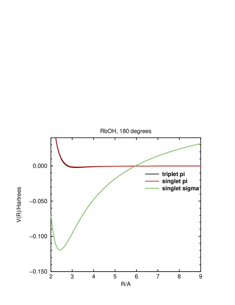
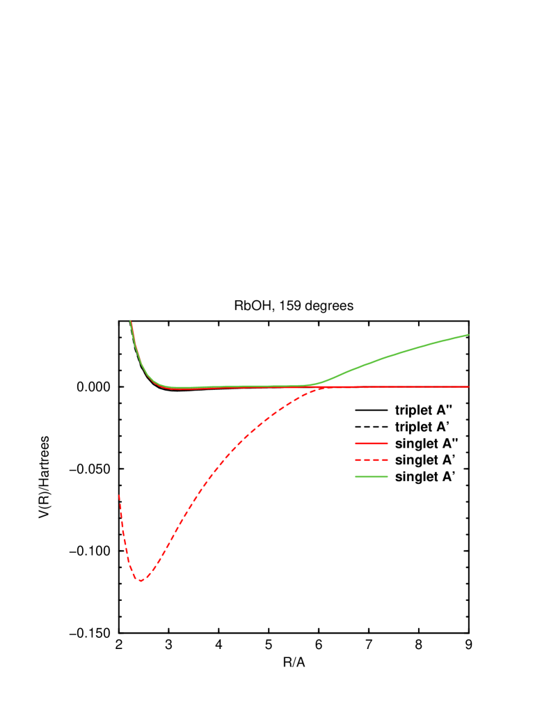
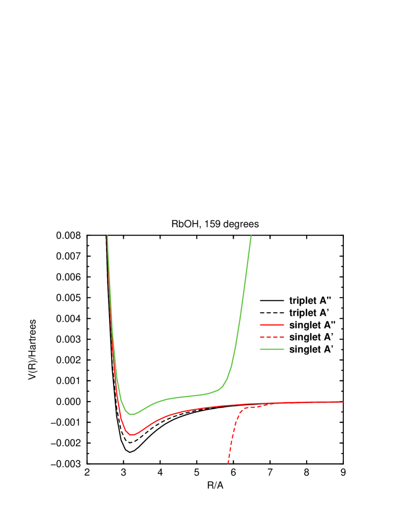
Figure 1: RbOH adiabatic potential curves from MRCI calculations, showing crossing for the Rb-OH linear geometry (a) and avoided crossing for a slightly nonlinear geometry ($\theta=159^{\circ}$, (b)). Panel (c) shows an expanded view of the curves in the center panel.

The ${}^{1}A^{\prime}$ electronic wavefunctions near the conical intersection are made up from two quite different configurations, so that a multiconfiguration electronic structure approach is essential to describe them. We have therefore chosen to use MCSCF (multiconfiguration self-consistent field) calculations followed by MRCI (multireference configuration interaction) calculations to characterize the surfaces. The electronic structure calculations initially produce adiabatic (Born-Oppenheimer) surfaces, but these are unsuitable for dynamics calculations both because they are difficult to interpolate (with derivative discontinuities at the conical intersections) and because there are nonadiabatic couplings between them that become infinite at the conical intersections. We have therefore transformed the two ${}^{1}A^{\prime}$ adiabatic surfaces that cross into a diabatic representation, where there are non-zero couplings between different surfaces but both the potentials and the couplings are smooth functions of coordinates.

The electronic structure calculations are carried out using the MOLPRO package MOLPRO . It was necessary to carry out an RHF (restricted Hartree-Fock) calculation to provide initial orbital guesses before an MCSCF calculation. It is important that the Hartree-Fock calculation gives good orbitals for both the OH $\pi$ and Rb 5s orbitals at all geometries (even those inside the crossing, where the Rb 5s orbital is unoccupied in the ground state). In addition, it is important that the OH $\pi$ orbitals are doubly occupied in the RHF calculations, as otherwise they are non-degenerate at linear geometries at the RHF level, and the MCSCF calculation is unable to recover the degeneracy. To ensure this, we begin with an RHF calculation on RbOH^- rather than neutral RbOH.

For Rb, we use the small-core quasirelativistic effective core potential (ECP) ECP28MWB ECPs with the valence basis set from Ref. Sol03 . This treats the 4s, 4p and 5s electrons explicitly, but uses a pseudopotential to represent the core orbitals. For O and H, we use the aug-cc-pVTZ correlation-consistent basis sets of Dunning Dunning in uncontracted form. Electronic structure calculations were carried out at 275 geometries, constructed from all combinations of 25 intermolecular distances $R$ and 11 angles $\theta$ in Jacobi coordinates. The 25 distances were from 2.0 to 6.0 Å in steps of 0.25 Å, from 6.0 to 9.0 Å in steps of 0.5 Å and from 9 Å to 12 Å in steps of 1 Å. The OH bond length was fixed at $r=0.9706$ Å. The 11 angles were chosen to be Gauss-Lobatto quadrature points Lobatto , which give optimum quadratures to project out the Legendre components of the potential while retaining points at the two linear geometries. The linear points are essential to ensure that the $A^{\prime}$ and $A^{\prime\prime}$ surfaces are properly degenerate at linear geometries: if we used Gauss-Legendre points instead, the values of the $A^{\prime}$ and $A^{\prime\prime}$ potentials at linear geometries would depend on extrapolation from nonlinear points and would be non-degenerate. The Gauss-Lobatto points correspond approximately to $\theta=0$, 20.9, 38.3, 55.6, 72.8, 90, 107.2, 124.4, 141.7, 159.1 and 180^∘, where $\theta=0$ is to the linear Rb-HO geometry. The calculations were in general carried out as angular scans at each distance, since this avoided most convergence problems due to sudden changes in orbitals between geometries.

II.1 Singlet states

We carried out a state-averaged MCSCF calculation of the lowest 3 singlet states of neutral RbOH (two ${}^{1}A^{\prime}$ and one ${}^{1}A^{\prime\prime}$). Molecular orbital basis sets will be described using the notation $(n_{A^{\prime}},n_{A^{\prime\prime}})$, where the two integers indicate the number of $A^{\prime}$ and $A^{\prime\prime}$ orbitals included. The orbital energies are shown schematically in Figure 2. The MCSCF basis set includes a complete active space (CAS) constructed from the lowest (10,3) molecular orbitals, with the lowest (5,1) orbitals closed (doubly occupied in all configurations). The MCSCF calculation generates a common set of orbitals for the 3 states. The calculations were carried out in $C_{s}$ symmetry, but at linear geometries the two components of the $\Pi$ states are degenerate to within our precision ($10^{-8}\,E_{h}$).

Figure 2: Schematic representation of the RbOH molecular orbitals from MCSCF calculations.

For cold molecule collisions, it is very important to have a good representation of the long-range forces. These include a large contribution from dispersion (intermolecular correlation), so require a correlated treatment. We therefore use the MCSCF orbitals in an MRCI calculation, again of the lowest three electronic states. The MOLPRO package implements the “internally contracted” MRCI algorithm of Werner and Knowles Wer . The reference space in the MRCI is the same as the active space for the MCSCF, and single and double excitations are included from all orbitals except oxygen 1s. As described in Appendix 1, the two ${}^{1}A^{\prime}$ states are calculated in a single MRCI block, so that they share a common basis set.

We encountered difficulties with non-degeneracy between the two components of the ${}^{1}\Pi$ states at linear geometries. These are described in Appendix 1. However, using the basis sets and procedures described here, the non-degeneracies were never greater than 90 $\mu E_{h}$ in the total energies for distances $R\geq 2.25$ Å (and considerably less in the interaction energies around the linear minimum).

II.2 Transforming to a diabatic representation

As described above, the two surfaces of ${}^{1}A^{\prime}$ symmetry cross at conical intersections at linear geometries. For dynamical calculations, it is highly desirable to transform the adiabatic states into diabatic states (or, strictly, quasidiabatic states). MOLPRO contains code to carry out diabatization by maximizing overlap between the diabatic states and those at a reference geometry. However, this did not work for our application because we were unable to find reference states that had enough overlap with the lowest adiabats at all geometries. We therefore adopted a different approach, based on matrix elements of angular momentum operators. We use a Cartesian coordinate system with the $z$ axis along the OH bond. At any linear geometry, the $\Pi$ component of ${}^{1}A^{\prime}$ symmetry is uncontaminated by the ion-pair state, and the matrix elements of $\hat{L}_{z}$ are

$$\langle^{1}A^{\prime}(\Pi)|\hat{L}_{z}|^{1}A^{\prime\prime}\rangle = i;$$

$$\langle^{1}A^{\prime}(\Sigma)|\hat{L}_{z}|^{1}A^{\prime\prime}\rangle = 0.$$ (1)

At nonlinear geometries, the actual ${}^{1}A^{\prime}$ states can be represented approximately as a mixture of $\Sigma$ and $\Pi$ components,

$$\left(\begin{matrix}\Psi_{1A^{\prime}}&\Psi_{2A^{\prime}}\end{matrix}\right)=\left(\begin{matrix}\Psi_{\Pi}&\Psi_{\Sigma}\end{matrix}\right)\left(\begin{matrix}\cos\phi&\sin\phi\\ -\sin\phi&\cos\phi\end{matrix}\right),$$ (2)

where the “singlet” superscripts have been dropped to simplify notation. If Eq. 2 were exact, the matrix elements of $\hat{L}_{z}$ would be

$$\langle 1A^{\prime}|\hat{L}_{z}|A^{\prime\prime}\rangle = i\cos\phi;$$

$$\langle 2A^{\prime}|\hat{L}_{z}|A^{\prime\prime}\rangle = i\sin\phi.$$ (3)

The mixing angle $\phi$ would thus be given by

$$\phi=\tan^{-1}\frac{\langle 2A^{\prime}|\hat{L}_{z}|A^{\prime\prime}\rangle}{\langle 1A^{\prime}|\hat{L}_{z}|A^{\prime\prime}\rangle}.$$ (4)

In the present work, we have taken the mixing angle to be defined by Eq. 4, using matrix elements of $\hat{L}_{z}$ calculated between the MRCI wavefunctions. This gives a mixing angle that, for linear geometries, is $\phi=0$ at long range and $\phi=\pi/2$ at short range (inside the crossing).

One complication that arises here is that the signs of the three wavefunctions are arbitrary, and may change discontinuously from one geometry to another. The signs of the matrix elements obtained numerically by MOLPRO are thus completely arbitrary. It was therefore necessary to pick a sign convention for the matrix elements at linear geometries and adjust the signs at other geometries to give a smoothly varying mixing angle.

It should be noted that this diabatization procedure is not general, and will fail if there is any geometry where both the numerator and the denominator of Eq. 4 are small. Fortunately, this was not encountered for RbOH. The sum of squares of the two matrix elements of $\hat{L}_{z}$ was never less than 0.99 at distances from $R=3.0$ Å outwards, and never less than 0.7 even at $R=2.0$ Å.

The mixing angles obtained for the singlet states of RbOH are shown as a contour plot in Figure 3. As expected, $\phi$ changes very suddenly from 0 to $90^{\circ}$ at linear and near-linear geometries, but smoothly at strongly bent geometries.

Figure 3: Contour plot of the diabatic mixing angle $\phi$ (in degrees) for the ${}^{1}A^{\prime}$ states of RbOH

Once a smooth mixing angle has been determined, the diabatic potentials and coupling surface are obtained from

$$\left(\begin{matrix}H_{11}&H_{12}\\ H_{21}&H_{22}\end{matrix}\right) = \left(\begin{matrix}\cos\phi&\sin\phi\cr-\sin\phi&\cos\phi\end{matrix}\right)$$ (5)

$$\times \left(\begin{matrix}E_{1A^{\prime}}&0\\ 0&E_{2A^{\prime}}\end{matrix}\right)\left(\begin{matrix}\cos\phi&-\sin\phi\\ \sin\phi&\cos\phi\end{matrix}\right).$$

Figure 4: Contour plot of the diabatic ${}^{1}A^{\prime}$ (panel (a)) and ${}^{1}A^{\prime\prime}$ (panel (b)) covalent (non-ion-pair) potential energy surfaces for RbOH from MRCI calculations. Contours are labeled in cm^-1.

Figure 5: Contour plot of the ${}^{1}A^{\prime}$ diabatic ion-pair potential energy surface (panel (a)) and the diabatic coupling potential (panel (b)) for RbOH from MRCI calculations. Contours are labeled in cm^-1.

The diabatization was carried out using total electronic energies (not interaction energies). The two singlet diabatic PES that correlate with Rb(${}^{2}S$) + OH(${}^{2}\Pi$) are shown in Figure 4, and the diabatic ion-pair surface and the coupling potential are shown in Figure 5. Some salient characteristics of the surfaces are given in Table 1. As required, the ${}^{1}A^{\prime\prime}$ and ${}^{1}A^{\prime}$ covalent states are degenerate at the two linear geometries, with a relatively deep well (337 cm^-1) at Rb-OH and a much shallower well at Rb-HO. At bent geometries, it is notable that the potential well is broader and considerably deeper for the ${}^{1}A^{\prime\prime}$ state than for the ${}^{1}A^{\prime}$ state; indeed, the ${}^{1}A^{\prime}$ state has a linear minimum, while the ${}^{1}A^{\prime\prime}$ has a bent minimum at $\theta=128^{\circ}$ with a well depth of 405 cm^-1. In spectroscopic terms, this corresponds to a Renner-Teller effect of type 1(b) in the classification of Pople and Longuet-Higgins Pop58 .

Table 1: Characteristics of the diabatic PES for RbOH.

		${}^{3}A^{\prime\prime}$	${}^{3}A^{\prime}$	${}^{1}A^{\prime\prime}$	${}^{1}A^{\prime}$	${}^{1}A^{\prime}$
					covalent	ion-pair
well depth/cm-1		615	511	405	337	26260
distance of minimum/Å		3.185	3.170	3.226	3.230	2.407
angle of minimum/ ∘		123	180	128	180	180

The fact that the ${}^{1}A^{\prime\prime}$ state is deeper than the ${}^{1}A^{\prime}$ state is somewhat unexpected, and will be discussed in more detail in the context of the triplet surfaces below. The fact that the surface for the covalent ${}^{1}A^{\prime}$ state is slightly repulsive between $R=4$ and 9 Å and between $\theta=40^{\circ}$ and $150^{\circ}$ is an artifact of the diabatization procedure and should not be given physical significance: the choice of mixing angle (4) is an approximation, and a slightly different choice would give different diabats and coupling terms, but of course corresponding to the same adiabatic surfaces.

The ion-pair state has a deep well at the RbOH geometry and a rather shallower one at RbHO, as expected from electrostatic considerations. The region around the minimum of this surface has been characterized in more detail by Lee and Wright Lee03 .

It is notable that the coupling potential is quite large, peaking at 2578 cm^-1 at $R=3.87$ Å and $\theta=83^{\circ}$, and is thus larger than the interaction energy for the two covalent surfaces at most geometries. It may be seen from Figure 3 that the $\Sigma-\Pi$ mixing it induces is significant at most distances less than 8 Å.

II.3 Triplet states

The triplet states of RbOH are considerably simpler than the singlet states, because there is no low-lying triplet ion-pair state. There is thus no conical intersection, and diabatization is not needed.

Single-reference calculations would in principle be adequate for the triplet states. Nevertheless, for consistency with the singlet surfaces, we carried out MCSCF and MRCI for the triplet surfaces as well. The (10,3) active and reference spaces were specified as for the singlet states, except that there is only one relevant ${}^{3}A^{\prime}$ state and the state average in the MCSCF calculation is therefore over the lowest two states.

Figure 6: Contour plot of the ${}^{3}A^{\prime}$ (panel (a)) and ${}^{3}A^{\prime\prime}$ (panel (b)) PES for RbOH from MRCI calculations. Contours are labeled in cm^-1.

Contour plots of the ${}^{3}A^{\prime}$ and ${}^{3}A^{\prime\prime}$ surfaces are shown in Figure 6. As for the singlet states, it is notable that the ${}^{3}A^{\prime\prime}$ state lies below the ${}^{3}A^{\prime}$ state at nonlinear geometries. This ordering is different from that found for systems such as Ar-OH Esp90 ; H93ArOH and He-OH Lee00 . In each case, the $A^{\prime}$ state corresponds to an atom approaching OH in the plane of the unpaired electron, while the $A^{\prime\prime}$ state corresponds to an atom approaching OH out of the plane. For He-OH and Ar-OH, the ${}^{2}A^{\prime}$ state is deeper than the ${}^{2}A^{\prime\prime}$ state simply because there is slightly less repulsion due to a half-filled $\pi$ orbital than due to a doubly filled $\pi$ orbital. Since these systems are dispersion-bound, and the dispersion coefficients are similar for the ${}^{2}A^{\prime}$ and ${}^{2}A^{\prime\prime}$ states, the slightly reduced repulsion for the ${}^{2}A^{\prime}$ state produces a larger well depth.

Rb-OH is quite different. The long-range coefficients still provide a large part of the binding energy of the covalent states, but the equilibrium distances (around 3.2 Å, Table 1) are about 1 Å shorter than would be expected from the sum of the Van der Waals radii of Rb (2.44 Å) and OH (1.78 Å, obtained from the Ar value of 1.88 Å and the Ar-OH equilibrium distance of 3.67 Å H93ArOH ).

The qualitative explanation is that at nonlinear geometries there is significant overlap between the Rb 5s orbital and the OH $\pi$ orbital of $a^{\prime}$ symmetry, forming weakly bonding and antibonding molecular orbitals (MOs) for the RbOH supermolecule. The effect of this is shown in Figure 7. In the $A^{\prime}$ states, the bonding and antibonding MOs are equally populated and there is no overall stabilization. However, for the $A^{\prime\prime}$ states the bonding MO is doubly occupied and the antibonding MO is singly occupied. This gives a significant reduction in the repulsion compared to a simple overlap-based model.

Even at linear Rb-OH geometries, the repulsion is reduced by a similar effect involving the Rb 5s orbital and the highest occupied OH $\sigma$ orbital ($6a^{\prime}$ in Figure 2).

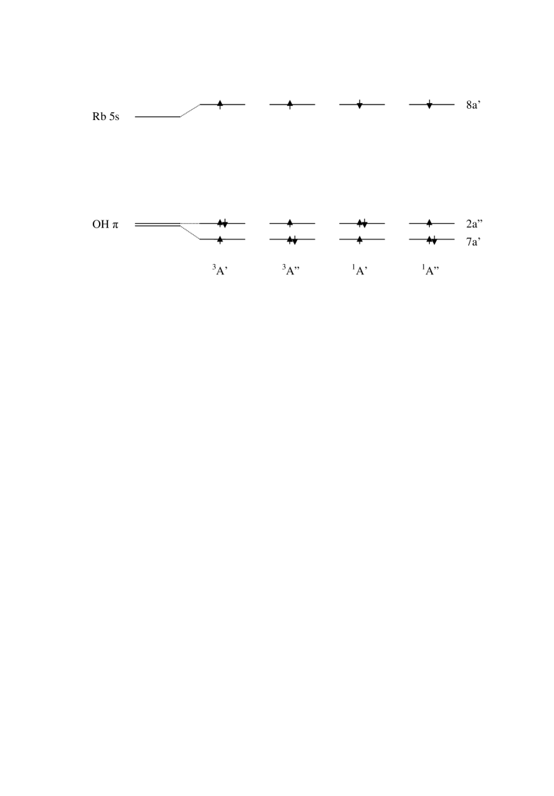
Figure 7: Orbital occupations for the covalent (non-ion-pair) states of RbOH at nonlinear geometries, $90^{\circ}<\theta<180^{\circ}$, showing the origin of the reduced repulsion for $A^{\prime\prime}$ states compared to $A^{\prime}$ states.

II.4 Converting MRCI total energies to interaction energies

The MRCI procedure is not size-extensive, so cannot be corrected for basis-set superposition error (BSSE) using the counterpoise approach Boy . In addition, there are Rb 5p orbitals that lie 1.87 eV above the ground state. This is below the ion-pair energy at large $R$, so that a (10,3) active space includes different orbitals asymptotically and at short range. It is thus hard to calculate asymptotic energies that are consistent with the short-range energies directly. Nevertheless, for collision calculations we ultimately need interaction energies, relative to the energy of free Rb(${}^{2}S$) + OH(${}^{2}\Pi$).

To circumvent this problem, we obtained angle-dependent long-range coefficients $C_{6}(\theta)$ and $C_{7}(\theta)$ for the triplet states of RbOH and used these to extrapolate from 12 Å outwards at each angle. We carried out RCCSD calculations (restricted coupled-cluster with single and double excitations) on the ${}^{3}A^{\prime}$ and ${}^{3}A^{\prime\prime}$ states at all angles at distances of 15, 25 and 100 Å. RCCSD was chosen in preference to RCCSD(T) for greater consistency with the MRCI calculations. Coupled cluster calculations are size-extensive, so in this case the interaction energies $V(R,\theta)$ for the ${}^{3}A^{\prime}$ and ${}^{3}A^{\prime\prime}$ states were calculated including the counterpoise correction Boy . The interaction energy at 100 Å was found to be non-zero (about $-1.38\,\mu E_{h}$), but was the same to within $10^{-9}\,E_{h}$ for both ${}^{3}A^{\prime}$ and ${}^{3}A^{\prime\prime}$ states and at all angles. For each pair of angles $\theta$ and $\pi-\theta$, the energies were fitted to the form

$$E(R,\theta)=E_{\infty}-C_{6}(\theta)R^{-6}-C_{7}(\theta)R^{-7}-C_{8}(\theta)R^{-8},$$ (6)

with the constraints that

$$C_{6}(\pi-\theta) = C_{6}(\theta)$$ (7)

$$C_{7}(\pi-\theta) = -C_{7}(\theta).$$ (8)

Sums and differences of the long-range coefficients for the two states,

$$C_{n}^{0}(\theta) = \frac{1}{2}\left[C_{n}^{A^{\prime\prime}}(\theta)+C_{n}^{A^{\prime}}(\theta)\right]$$ (9)

$$C_{n}^{2}(\theta) = \frac{1}{2}\left[C_{n}^{A^{\prime\prime}}(\theta)-C_{n}^{A^{\prime}}(\theta)\right],$$ (10)

were then smoothed by fitting to the theoretical functional forms

$$C_{6}^{0}(\theta) = C_{6}^{00}+C_{6}^{20}P_{2}^{0}(\cos\theta)$$ (11)

$$C_{6}^{2}(\theta) = C_{6}^{22}P_{2}^{2}(\cos\theta)$$ (12)

$$C_{7}^{0}(\theta) = C_{7}^{10}P_{1}^{0}(\cos\theta)+C_{7}^{30}P_{3}^{0}(\cos\theta)$$ (13)

$$C_{7}^{2}(\theta) = C_{7}^{32}P_{3}^{2}(\cos\theta),$$ (14)

where $P_{\lambda}^{\nu}(\cos\theta)$ are associated Legendre functions. The coefficients obtained by this procedure are summarized in Table 2. The resulting smoothed values of $C_{6}^{0}(\theta)$, $C_{6}^{2}(\theta)$, $C_{7}^{0}(\theta)$ and $C_{7}^{2}(\theta)$ were then used to generate $C_{6}^{A^{\prime}}(\theta)$, $C_{6}^{A^{\prime\prime}}(\theta)$, $C_{7}^{A^{\prime}}(\theta)$ and $C_{7}^{A^{\prime\prime}}(\theta)$. Finally, the MRCI total energies at $R=10$ and 12 Å for both singlet and triplet states were refitted to Eq. 6, with $C_{6}(\theta)$ and $C_{7}(\theta)$ held constant at the smoothed values, to obtain an MRCI value of $E_{\infty}$ for each angle (and surface). These angle-dependent values of $E_{\infty}$ were used to convert the MRCI total energies into interaction energies.

It should be noted that the long-range coefficients in Rb-OH have substantial contributions from induction as well as dispersion. A simple dipole-induced dipole model gives $C_{\rm 6,ind}^{00}=C_{\rm 6,ind}^{20}=133\ E_{h}a_{0}^{6}$ and accounts for 40% of $C_{\rm 6}^{00}$ and 90% of $C_{\rm 6}^{20}$

Table 2: Long-range coefficients for Rb-OH obtained by fitting to RCCSD calculations on triplet states.

$\lambda$	0	1	2	3
$C_{6}^{\lambda 0}/E_{h}a_{0}^{6}$	325.0	–	151.0	–
$C_{6}^{\lambda 2}/E_{h}a_{0}^{6}$	–	–	1.9	–
$C_{7}^{\lambda 0}/E_{h}a_{0}^{7}$	–	1035.4	–	630.0
$C_{7}^{\lambda 2}/E_{h}a_{0}^{7}$	–	–	–	–40.1

II.5 Interpolation and fitting

The procedures described above produce six potential energy surfaces on a two-dimensional grid of geometries $(R,\theta)$: four surfaces corresponding to covalent states (“c”), with $A^{\prime}$ or $A^{\prime\prime}$ symmetry and triplet or singlet multiplicity, one surface with ion-pair character with ${}^{1}A^{\prime}$ symmetry, and finally the non-vanishing coupling of this latter state with the covalent ${}^{1}A^{\prime}$ state. We will denote the 6 surfaces $V^{{}^{1}A^{\prime}_{\rm c}}$, $V^{{}^{1}A^{\prime\prime}_{\rm c}}$, $V^{{}^{3}A^{\prime}_{\rm c}}$, $V^{{}^{3}A^{\prime\prime}_{\rm c}}$, $V^{{}^{1}A^{\prime}_{\rm i}}$, and $V^{\rm ic}$, respectively. Labels will be dropped below when not relevant to the discussion.

For the covalent states of each spin multiplicity, interpolation was carried out on sum and difference potentials,

$$V_{0}(R,\theta) = \frac{1}{2}\left[V^{A^{\prime\prime}}(R,\theta)+V^{A^{\prime}}(R,\theta)\right]$$ (15)

$$V_{2}(R,\theta) = \frac{1}{2}\left[V^{A^{\prime\prime}}(R,\theta)-V^{A^{\prime}}(R,\theta)\right],$$ (16)

with the difference potentials set to zero at $\theta=0$ and $180^{\circ}$ to suppress the slight non-degeneracy in the MRCI results. Our approach to two-dimensional interpolation follows that of Meuwly and Hutson H99NeHFmorph and Soldán et al. Soljcp02a . The interpolation was carried out first in $R$ (for each surface and angular point) and then in $\theta$. The interpolation in $R$ used the RP-RKHS (reciprocal power reproducing kernel Hilbert space) procedure Ho96 with parameters $m=5$ and $n=3$. This gives a potential with long-range form

$$V_{q}(R,\theta)=-C_{6}^{q}(\theta)R^{-6}-C_{7}^{q}(\theta)R^{-7}-C_{8}^{q}(\theta)R^{-8}.$$ (17)

The values of $C_{6}^{q}(\theta)$ and $C_{7}^{q}(\theta)$ were fixed at the values described in the previous subsection Ho00 ; Sol00 .

For the ion-pair state, it is the quantity $V^{\rm i}(R,\theta)-E_{\infty}^{\rm i}$ that is asymptotically zero, where $E_{\infty}^{\rm i}=0.0863426\,E_{h}$ is the ion-pair threshold. This was interpolated using RP-RKHS interpolation with parameters $m=0$ and $n=2$, which gives a potential with long-range form

$$V^{\rm i}(R,\theta)=E_{\infty}^{\rm i}-C_{1}(\theta)R^{-1}-C_{2}(\theta)R^{-2}.$$ (18)

The coefficient $C_{1}(\theta)$ was fixed at the Coulomb value of $1\,E_{h}a_{0}^{-1}$.

The coupling potential $V^{\rm ic}(R,\theta)$ has no obvious inverse-power form at long range. It was therefore interpolated using the ED-RKHS (exponentially decaying RKHS) approach Hol99 , with $n=2$ and $\beta=0.77$ Å. This gives a potential with long-range form

$$V^{\rm ic}(R,\theta)=A(\theta)\exp(-\beta R).$$ (19)

The value of $\beta$ was chosen by fitting the values of the coupling potential at $R=10$ and 12 Å to decaying exponentials.

Interpolation in $\theta$ was carried out in a subsequent step. An appropriate angular form is

$$V_{q}(R,\theta)=\sum_{k}V_{kq}(R)\Theta_{kq}(\cos\theta),$$ (20)

where $\Theta_{kq}(\cos\theta)$ are normalized associated Legendre functions,

$$\Theta_{kq}(\cos\theta)=\sqrt{\left(\frac{2k+1}{2}\right)\frac{(k-|q|)!}{(k+|q|)!}}P_{k}^{|q|}(\cos\theta),$$ (21)

and $q=0$ for the sum and ion-pair potentials, 2 for the difference potentials and 1 for the coupling potential. $q$ can thus be used as a label to distinguish the different potentials. The coefficients $V_{kq}(R)$ for $k=q$ to 9 were projected out using Gauss-Lobatto quadrature, with weights $w_{i}$,

$$V_{kq}(R)=\sum_{i}w_{i}V_{q}(R,\theta_{i})\Theta_{kq}(\cos\theta_{i}),$$ (22)

Since there are fewer coefficients than points, the resulting potential function does not pass exactly through the potential points. However, the error for the covalent states in the well region is no more than 20 $\mu E_{h}$.

We thus arrive at a set of $R$-dependent coefficients $V_{kq}^{\alpha,2S+1}(R)$, with $\alpha={\rm c}$, i or ic labeling the potentials for the pure covalent or ion-pair states or the coupling between them and $2S+1=0$ or 1 for singlet or triplet states respectively. These coefficients will be used below in evaluating the electronic potential matrix elements which couple collision channels in the dynamical calculations.

III Dynamical methodology

III.1 The basis sets

We carry out coupled-channel calculations of the collision dynamics. The channels are labeled by quantum numbers that characterize the internal states of the colliding partners, plus partial wave quantum numbers that define the way the partners approach each other.

It is convenient to distinguish between the laboratory frame, whose $z$ axis is taken to be along the direction of the external field (if any) and the molecule frame, whose $z$ axis lies along the internuclear axis of the OH molecule and whose $xz$ plane contains the triatomic system. This allows us to define external coordinates that fix the collision plane, and internal coordinates that describe the relative position of the components on it. As external coordinates, we choose the Euler angles $(\alpha,\beta,\gamma)$ required to change from the laboratory frame to the molecule-frame; as internal coordinates we use the system of Jacobi coordinates ($R,\theta$) defined above. We also define the spherical angles ($\theta^{\prime},\phi^{\prime}$) that describe the orientation of the intermolecular axis in the external (laboratory) frame.

We first focus on the covalent channels OH$(\pi^{3},\ ^{2}\Pi)+{\rm Rb}(5s^{1},\ ^{2}S_{1/2})$. The OH molecule can be described using Hund’s case (a) quantum numbers: the internal state is expressed in a basis set given by $|s_{d}\sigma\rangle|\lambda\rangle|jm\omega\rangle$, where $s_{d}$ is the electronic spin of OH and $\sigma$ its projection on the internuclear axis; $\lambda$ is the projection of the electronic orbital angular momentum onto the internuclear axis; $j$ is the angular momentum resulting from the electronic and rotational degrees of freedom, $m$ its projection on the laboratory axis and $\omega=\lambda+\sigma$ its projection on the internuclear axis. The symmetric top wavefunctions that describe the rotation of the diatom in space are defined by $|jm\omega\rangle=\sqrt{\frac{2j+1}{8\pi^{2}}}D_{m\omega}^{j*}(\alpha,\beta,\gamma)$. At this stage $\lambda$, $\sigma$ and $\omega$ are still signed quantities. However, in zero electric field, energy eigenstates of OH are also eigenstates of parity, labeled $\epsilon=e$ or $f$. These labels refer to “+“or “$-$” sign taken in the combination of $\omega$ and $-\omega$; the real parity is given by $\epsilon(-1)^{j-s_{d}}$. To include parity, we can define states $|s_{d}\bar{\lambda}\bar{\omega}\epsilon jm\rangle$, where the bar indicates the absolute values of a signed quantity. Finally, we need to include also the nuclear spin degree of freedom: if $i_{d}$ designates the nuclear spin angular momentum of the diatom, then $j$ and $i_{d}$ combine to form $f_{d}$, the total angular momentum of the diatom, which has projection $m_{f_{d}}$ on the laboratory $z$ axis. The resulting basis set that describes the physical states of the OH molecule is

$$|s_{d}\bar{\lambda}\bar{\omega}\epsilon(ji_{d})f_{d}m_{f_{d}}.\rangle$$ (23)

For Rb, the electronic angular momentum is given entirely by the spin $s_{a}$ of the open-shell electron, which combines with the nuclear spin $i_{a}$ to form $f_{a}$, the total angular momentum of the atom. The state of the Rb atom can then be expressed as

$$|(s_{a}i_{a})f_{a}m_{f_{a}}\rangle.$$ (24)

The explicit inclusion of the $s_{d}$ and $s_{a}$ quantum numbers allows us to use the same notation for ion-pair channels OH${}^{-}(\pi^{4},\ ^{1}\Sigma^{+})+{\rm Rb}^{+}(^{1}S_{0})$: in this case both partners are closed-shell, so $s_{d}=s_{a}=\bar{\lambda}=\bar{\omega}=0$ and $\epsilon=+1$.

The resulting basis set for close-coupling calculations on the complete system (designated B1) has the form

$$|B1\rangle=|s_{d}\bar{\lambda}\bar{\omega}\epsilon(ji_{d})f_{d}m_{f_{d}}\rangle|(s_{a}i_{a})f_{a}m_{f_{a}}\rangle|LM_{L}\rangle,$$ (25)

where $|LM_{L}\rangle$ denotes the partial wave degree of freedom and is a function of the $(\theta^{\prime},\phi^{\prime})$ coordinates considered above. The ket $|LM_{L}\rangle$ corresponds to $Y_{LM_{L}}(\theta^{\prime},\phi^{\prime})$. Ultimately, S-matrix elements for scattering are expressed in basis set B1.

The scattering Hamiltonian is block-diagonal in total angular momentum and total parity. The total parity is well defined in the basis set we have selected, and given by $p=\epsilon(-1)^{j-s_{d}+L}$. It is conserved in the presence of a magnetic field but not an electric field. The total angular momentum is not conserved in the presence of either a magnetic or an electric field. However, the projection of total angular momentum on the laboratory $z$ axis, given by $M_{\mathcal{J}}=m_{f_{d}}+m_{f_{a}}+M_{L}$, is conserved in the presence of an external field aligned with the laboratory $z$ axis.

III.2 Matrix elements of the potential energy

The PES in section II are diagonal in the total electronic spin, $S$, and in the states of the nuclei, $m_{i_{a}}$ and $m_{i_{d}}$, with $m_{i_{a}}$ and $m_{i_{d}}$ the nuclear spin projections of the atom and diatom in the laboratory frame. We therefore find it convenient to define basis sets labeled by these quantum numbers. This allows not only the direct calculation of potential matrix elements, but the definition of some useful frame transformations Fano . Two other basis sets, B2 and B3, defined with/without parity (B2p/B2w and B3p/B3w) are described in Appendix 2. The corresponding frame transformations are defined in section III.3.

The calculation of the matrix elements of the potential energy is most direct in basis set B2w. This is based on Hund’s case (b) quantum numbers for the molecule, and is given by

$$|B2w\rangle=|(s_{d}s_{a})SM_{S}\rangle|nm_{n}\lambda\rangle|i_{d}m_{i_{d}}\rangle|i_{a}m_{i_{a}}\rangle|LM_{L}\rangle,$$ (26)

where $n$ is the total angular momentum excluding spin, with projection $\lambda$ on the internuclear axis, $|SM_{S}\rangle$ indicates the total spin state of the electrons, and $|i_{a}m_{i_{a}}\rangle|i_{d}m_{i_{d}}\rangle$ indicates the states of the nuclei.

In order to relate the PES obtained in section II to the quantum numbers of our channels, it is convenient to recast the electronic wavefunctions for the covalent states of ${}^{2S+1}A^{\prime}$ and ${}^{2S+1}A^{\prime\prime}$ in terms of functions with definite values of $\lambda$,

$$|^{1(3)}{+1}_{\rm c}\rangle =-\frac{1}{\sqrt{2}}(|^{1(3)}A^{\prime}_{\rm c}\rangle+i|^{1(3)}A^{\prime\prime}_{\rm c}\rangle);$$

$$|^{1(3)}{-1}_{\rm c}\rangle =\frac{1}{\sqrt{2}}(|^{1(3)}A^{\prime}_{\rm c}\rangle-i|^{1(3)}A^{\prime\prime}_{\rm c}\rangle).$$ (27)

We can also associate $\lambda=0$ with the ion-pair wavefunction (and denote it $|^{1}0_{\rm i}\rangle$). Then the multipole index $q$ in the potential expansion (20) is viewed as an angular momentum transfer $q=\lambda^{\prime}-\lambda$.

The B2w basis functions do not explicitly depend on $\theta$. We therefore rotate the $\Theta_{kq}$ functions Brink onto the laboratory frame, to which molecular spins and partial waves are ultimately referred. The functions $\Theta_{kq}$ are proportional to renormalized spherical harmonics $C_{kq}(\theta,0)$ Brink , for which

$$C_{kq}(\theta,0)=\sum_{\nu}D_{\nu q}^{k}(\alpha,\beta,\gamma)C_{k\nu}(\theta^{\prime},\phi^{\prime}).$$ (28)

The potential now depends on the same angular coordinates as the B2w basis functions. Integrating and applying the usual relationships, we obtain the matrix elements of the electronic potential in basis set $|B2w\rangle$,

$$\langle LM_{L}|\langle(s_{d}s_{a})SM_{S}|\langle nm_{n}\lambda|V|n^{\prime}m^{\prime}_{n}\lambda^{\prime}\rangle|(s^{\prime}_{d}s^{\prime}_{a})S^{\prime}M^{\prime}_{S}\rangle|L^{\prime}M^{\prime}_{L}\rangle$$ (38)

$$=\delta_{SS^{\prime}}\delta_{M_{S}M^{\prime}_{S}}\sum_{k}\sqrt{[n][n^{\prime}][L][L^{\prime}]}(-1)^{(M_{L}+m^{\prime}_{n}-\lambda^{\prime})}\left(\begin{array}[]{ccc}L&k&L^{\prime}\\ -M_{L}&\nu&M_{L}^{\prime}\end{array}\right)\left(\begin{array}[]{ccc}L&k&L^{\prime}\\ 0&0&0\end{array}\right)$$

$$\times\left(\begin{array}[]{ccc}n&k&n^{\prime}\\ m_{n}&\nu&-m_{n}^{\prime}\end{array}\right)\left(\begin{array}[]{ccc}n&k&n^{\prime}\\ \lambda&q&-\lambda^{\prime}\end{array}\right)\sqrt{\frac{(2k+1)}{2}}\kappa V_{k|q|}^{\alpha,2S+1}(R),$$

where $[A]=2A+1$, $q=\lambda^{\prime}-\lambda$ and $\nu=m^{\prime}_{n}-m_{n}$. $\kappa$ is a constant whose value in the case of covalent-covalent or ionic-ionic matrix elements ($q=0,\pm 2$) is 1. For covalent-ionic or ionic-covalent matrix elements ($q=\pm 1$), $\kappa=-\sqrt{1/2}$ or $\kappa=\sqrt{1/2}$ respectively. In these last two cases, $V_{k|q|}^{\alpha,2S+1}(R)=V_{k1}^{\rm ic,1}(R)$.

Our aim is to evaluate the matrix elements of the potential in basis set B1. Basis set B3w, defined in Appendix 2, can be considered as an intermediate step between B2w and B1. Starting from Eq. 38 and changing basis to B3w (see Appendix 2), we obtain

$$\langle LM_{L}|\langle i_{a}m_{i_{a}}|\langle s_{a}m_{s_{a}}|\langle i_{d}m_{i_{d}}|\langle jm\omega|\langle\lambda|\langle s_{d}\sigma|V|s_{d}^{\prime}\sigma^{\prime}\rangle|\lambda^{\prime}\rangle|j^{\prime}m^{\prime}\omega^{\prime}\rangle|i^{\prime}_{d}m^{\prime}_{i_{d}}\rangle|s_{a}^{\prime}m^{\prime}_{s_{a}}\rangle|i^{\prime}_{a}m^{\prime}_{i_{a}}\rangle|L^{\prime}M_{L}^{\prime}\rangle$$

$$= \delta_{i_{a}i^{\prime}_{a}}\delta_{m_{i_{a}}m^{\prime}_{i_{a}}}\delta_{i_{d}i^{\prime}_{d}}\delta_{m_{i_{d}}m^{\prime}_{i_{d}}}\sum_{k}\sum_{m_{s_{d}}}\sum_{m^{\prime}_{s_{d}}}\sum_{S}(2S+1)\left(\begin{array}[]{ccc}s_{d}&s_{a}&S\\ m_{s_{d}}&m_{s_{a}}&-M_{S}\end{array}\right)\left(\begin{array}[]{ccc}s_{d}^{\prime}&s_{a}^{\prime}&S\\ m^{\prime}_{s_{d}}&m^{\prime}_{s_{a}}&-M_{S}\end{array}\right)$$

$$\times (-1)^{m+m^{\prime}-\omega-\omega^{\prime}+M_{L}+m^{\prime}_{n}-\lambda^{\prime}+j+j^{\prime}+n+n^{\prime}+s_{d}+s_{d}^{\prime}}\sqrt{[j][j^{\prime}][L][L^{\prime}]}\sum_{nn^{\prime}}[n][n^{\prime}]$$

$$\times \left(\begin{array}[]{ccc}j&s_{d}&n\\ m&-m_{s_{d}}&-m_{n}\end{array}\right)\left(\begin{array}[]{ccc}n&k&n^{\prime}\\ m_{n}&\nu&-m_{n}^{\prime}\end{array}\right)\left(\begin{array}[]{ccc}L&k&L^{\prime}\\ -M_{L}&\nu&M_{L}^{\prime}\end{array}\right)\left(\begin{array}[]{ccc}j^{\prime}&s_{d}^{\prime}&n^{\prime}\\ m^{\prime}&-m^{\prime}_{s_{d}}&-m_{n}^{\prime}\end{array}\right)$$ (52)

$$\times \left(\begin{array}[]{ccc}j&s_{d}&n\\ \omega&-\sigma&-\lambda\end{array}\right)\left(\begin{array}[]{ccc}n&k&n^{\prime}\\ \lambda&q&-\lambda^{\prime}\end{array}\right)\left(\begin{array}[]{ccc}L&k&L^{\prime}\\ 0&0&0\end{array}\right)\left(\begin{array}[]{ccc}j^{\prime}&s_{d}^{\prime}&n^{\prime}\\ \omega^{\prime}&-\sigma^{\prime}&-\lambda^{\prime}\end{array}\right)\sqrt{\frac{(2k+1)}{2}}\kappa V_{k|q|}^{\alpha,2S+1}(R).$$ (61)

The potential matrix elements in basis sets B2p and B3p are trivially related to the ones in B2w and B3w, respectively, requiring only the change to a parity-symmetrized basis set, built as a superposition of $+\lambda$ and $-\lambda$ or $+\omega$ and $-\omega$ vectors. Finally, the evaluation of the potential in basis set B1 can be easily obtained from that in B3p by taking the standard composition of $j$ and $s_{a}$ with the respective nuclear angular momenta $i_{d}$ and $i_{a}$.

The true eigenstates of OH are linear combinations of functions with different values of $\omega$, mixed by spin-uncoupling terms in the hamiltonian. The mixing is significant even for the rotational ground state: $85\%$ of $\omega=3/2$ and $15\%$ of $\omega=1/2$. We have approximated OH as a pure case (a) molecule for convenience in the present work. The fine and hyperfine energies, taken from the work of Coxon et al. Coxon , were associated to a unique set of case (a) quantum numbers $|s_{d}\bar{\lambda}\bar{\omega}\epsilon(ji_{d})f_{d}m_{f_{d}}\rangle$. For Rb, the experimental values are taken from ref. Arim, . Figure 8 shows the quantum numbers that characterize the internal states of the colliding partners for the 8 lowest asymptotic thresholds, corresponding to the rotational state $\bar{\omega}=3/2,j=3/2$ of OH.

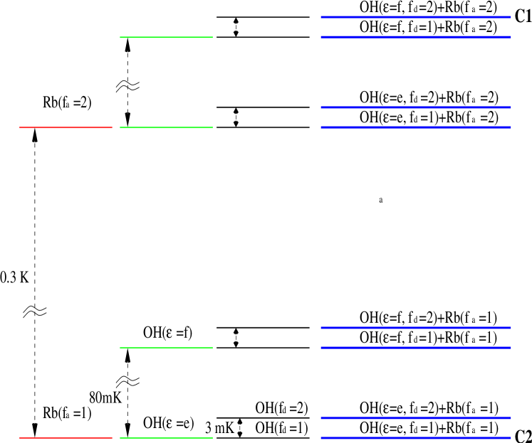
Figure 8: Threshold diagram for the channels of interest, labeled by quantum numbers that characterize the internal states of both colliding partners. These correspond to the ground rotational state $\bar{\omega}=3/2,j=3/2$ of OH. Thresholds corresponding to the incident channels considered in section IV (C1 and C2) are indicated. Hyperfine splitting in Rb and $\Lambda$-doubling and hyperfine splitting in OH are given.

III.3 Solving the Schrödinger equation

The full Hamiltonian operator can be written

$$\hat{H} = -{\hbar^{2}\over{2\mu}}\left[R^{-1}\left(\frac{\partial^{2}}{\partial R^{2}}\right)R-\frac{{\hat{L}}^{2}}{R^{2}}\right]+\hat{V}(R)+\hat{H}_{\rm th},$$ (62)

where $\mu$ is the reduced mass, $\hat{V}(R)$ indicates the potential matrix containing the electronic potential matrix elements given in the previous section and $\hat{H}_{\rm th}$ is the constant thresholds matrix. By construction, any constant difference of energy between channels has been relegated to the threshold matrix so that the potential matrix elements die off at long range.

The coupled-channel equations that result from introducing this Hamiltonian into the total Schrödinger equation are propagated using the log-derivative method of Johnson Johnson , modified to take variable step sizes keyed to the local de Broglie wavelength. The log-derivative matrix $Y$ thus obtained is matched to spherical Bessel functions in the usual way to yield the scattering matrix $S$. Using $T$ matrix elements ($T=i(S-1)$) Mott , the cross section for incident energy $E$ between internal states $\alpha$ and $\beta$, corresponding to a beam experiment, can be obtained using the expression

$$\sigma_{\alpha\rightarrow\beta}(E) = \sum_{LL^{\prime}M^{\prime}_{L}L^{\prime\prime}}\frac{\pi}{k^{2}}i^{L^{\prime\prime}-L}\sqrt{(2L+1)(2L^{\prime\prime}+1)}$$ (63)

$$\times T^{*}_{\alpha L0\rightarrow\beta L^{\prime}M^{\prime}_{L}}(E)T_{\alpha L^{\prime\prime}0\rightarrow\beta L^{\prime}M^{\prime}_{L}}(E),$$

where the collision axis is chosen along the quantization axis (so that only $M_{L}=0$ contributes). The labels $\alpha$ and $\beta$ designate sets of quantum numbers specifying the internal states of both colliding partners ($s_{d}\bar{\lambda}\bar{\omega}\epsilon(ji_{d})f_{d}m_{f_{d}},(s_{a}i_{a})f_{a}m_{f_{a}}$), and $k=(2\mu E/\hbar^{2})^{1/2}$ is the wave number corresponding to incident kinetic energy $E$.

Our aim is to extract information for collisional processes involving OH$(j=3/2,^{2}\Pi_{3/2})+{\rm Rb}(5s^{1},\ ^{2}S_{1/2})$, in any of their hyperfine states, with translational energies in the range $10^{-6}$ to $1$ K. This range comfortably includes both the temperatures currently reached in buffer-gas or Stark deceleration experiments and the target temperatures of sympathetic cooling. A fully converged calculation would require propagation to large values of $R$ and the inclusion of a huge number of channels. Although both covalent and ion-pair channels should be considered, in this pilot study we include only covalent states, except in Section IV.3 below. The large anisotropy of the surfaces included in the calculation makes it necessary to use a large number of OH rotational states and partial waves; the inclusion of rotational states up to $j=11/2$ is required (these states lie $\approx 550$ cm^-1 ($\bar{\omega}=3/2$) and $\approx 850$ cm^-1 ($\bar{\omega}=1/2$) above the ground state, numbers comparable to the depth of the covalent potential energy surfaces). The number of partial waves needed for convergence for each rotational state is shown in Table 3; it may be seen that fewer partial waves are required for higher rotational states. Unfortunately, a fully converged calculation was beyond our computational resources, so we reduced the number of channels to include only $40\%$ of those in Table 3. This gives cross sections accurate to within a factor of 2.

Table 3: Approximate number of partial waves required in a converged calculation for each rotational state ($\bar{\omega},j$).

	$j=1/2$	$j=3/2$	$j=5/2$	$j=7/2$	$j=9/2$	$j=11/2$
$\bar{\omega}=3/2$		70	70	60	50	25
$\bar{\omega}=1/2$	70	70	70	65	50	40

We consider first the collision of atoms and molecules that are both in their maximally stretched states, $(f_{a},m_{f_{a}})=(f_{d},m_{f_{d}})=(2,+2)$. The s-wave incident channel has $L=0$ and $M_{L}=0$, so corresponds to $M_{\mathcal{J}}=+4$. The set of all $M_{\mathcal{J}}=+4$ channels with a defined total parity $p$, including all allowed $M_{L}$ projections, as well as all the $f_{a}$, $f_{d}$, $m_{f_{a}}$ and $m_{f_{d}}$ quantum numbers (or equivalently $m$, $m_{s_{a}}$ and $m_{i_{a}}$, $m_{i_{d}}$) contains 23433 channels. This makes an exact calculation infeasible. We have therefore introduced two approximations to reduce this number. First, the projection $m_{f_{d}}$ for channels with $j>5/2$ is fixed to its initial value; the suppressed projections increase the degeneracy and might split rotational Feshbach resonances, but numerical tests show that making this approximation does not substantially alter the overall magnitude of the cross sections reported here. This approximation reduces the number of channels to 10555. Second, for propagation at large $R$ we disregard channels that are “locally closed”, that is, whose centrifugal barrier is higher than the incident energy in a given amount that is modified until converence.

Even with these approximations, and the suppression of ion-pair channels, it is impractical to perform full calculations. However, dividing the radial solution of the Schrödinger equation into an inner region ($R<R_{0}$) and an outer region ($R>R_{0}$) makes it possible to use different basis sets (“frames”) in each of them. Frame transformations have previously been employed for the simpler problem of alkaline earth+alkaline earth collisions Burke and for electron-molecule collisions Fano . They will be an essential tool for introducing hyperfine structure into atom-molecule and molecule-molecule collision problems Nueva . The calculation is thus divided into two different steps:

• At short range, $R<R_{0}$, the hyperfine interaction is small compared to the depths of the short-range potentials. We therefore represent the Hamiltonian in basis set B3 (see Appendix 2), where the potential is diagonal in nuclear spin projections $m_{i_{a}}$ and $m_{i_{d}}$. There are 8 such blocks (since $(2i_{d}+1)(2i_{a}+1)=8$). We ignore elements of $\hat{H}_{\rm th}$ that couple different pairs of $m_{i_{a}}$ and $m_{i_{d}}$. This reduces a single $(8N)\times(8N)$ calculation to 8 $(N\times N)$ calculations. At $R=R_{0}$ the complete $Y$ matrix can be rebuilt using the partial $Y_{m_{i_{a}},m_{i_{d}}}$ matrices obtained from each subset, $|s_{d}\bar{\lambda}\bar{\omega}\epsilon jm\rangle|s_{a}m_{a}\rangle|LM_{L}\rangle$

  $$\langle LM_{L}|\langle i_{a}m_{i_{a}}|\langle s_{a}m_{s_{a}}|\langle i_{d}m_{i_{d}}|\langle s_{d}\bar{\lambda}\bar{\omega}\epsilon jm|Y|s^{\prime}_{d}\bar{\lambda}^{\prime}\bar{\omega}^{\prime}\epsilon^{\prime}j^{\prime}m^{\prime}\rangle|i_{d}^{\prime}m_{i_{d}}^{\prime}\rangle|s_{a}^{\prime}m^{\prime}_{s_{a}}\rangle|i_{a}^{\prime}m^{\prime}_{i_{a}}\rangle|L^{\prime}M_{L}^{\prime}\rangle$$ (64)

  $$= \delta_{i_{a}i^{\prime}_{a}}\delta_{m_{i_{a}}m^{\prime}_{i_{a}}}\delta_{i_{d}i^{\prime}_{d}}\delta_{m_{i_{d}}m^{\prime}_{i_{d}}}\langle LM_{L}|\langle s_{a}m_{s_{a}}|\langle s_{d}\bar{\lambda}\bar{\omega}\epsilon jm|Y_{m_{i_{a}},m_{i_{d}}}|s^{\prime}_{d}\bar{\lambda}^{\prime}\bar{\omega}^{\prime}\epsilon^{\prime}j^{\prime}m^{\prime}\rangle|s_{a}^{\prime}m^{\prime}_{s_{a}}\rangle|L^{\prime}M_{L}^{\prime}\rangle.$$

  This $Y$ matrix is then transformed into the asymptotic basis set B1. We have found that this frame transform provides a very accurate way to include the Rb-OH hyperfine structure in reduced calculations using only covalent channels. Moreover, owing to the depth of the short-range potentials, $Y$ is weakly dependent on energy and can be interpolated in the inner region.

• At long range, $R>R_{0}$, the $Y$ matrix, expressed already in B1, is propagated to large distances to obtain the $S$ matrix. We invoke an alternative approximation: The coupling between different asymptotic rotational and fine-structure states diminishes at longer distances and can be neglected. Thus the subset corresponding to the ground rotational diatomic state ($j=3/2$, $\bar{\omega}=3/2$) can be propagated by itself to asymptotic distances. We reinstate the full hyperfine Hamiltonian in this region.

It is worth noting that basis set B2, defined in Appendix 2, could also be the basis for another frame transformation. Approximate decoupling of singlet and triplet channels in the inner region would allow a partition of the numerical effort into two smaller groups of channels, and the introduction of the ionic channels in the singlet one.

IV Scattering cross sections

We have calculated elastic and state-resolved inelastic cross sections for two different incident channels for collisions of Rb atoms with OH molecules. These are shown as C1 and C2 in Figure 8. Although we do not include the effects of external fields explicitly in this work, we consider states in which both partners can be in weak-field-seeking states in a magnetic field, and thus magnetically trappable. The OH hyperfine states that can be trapped at laboratory magnetic fields are $(f_{d}=2,m_{f_{d}}=+2,+1,0)$ and $(f_{d}=1,m_{f_{d}}=+1)$, while the corresponding states for Rb are $(f_{a}=2,m_{f_{a}}=+2,+1,0)$; the Rb state $(f_{a}=1,m_{f_{a}}=-1)$ is trappable for fields smaller that $\approx 1250$ gauss.

In the first case, designated C1 in Figure 8, both partners are in maximally stretched states: OH$(\epsilon=f,f_{d}=2,m_{f_{d}}=2)$ + Rb$(f_{a}=2,m_{f_{a}}=2)$. This case corresponds to the highest threshold correlating with OH in its ground rotational state. In this case, OH is also electrostatically trappable. The second case, designated C2 in Figure 8, correlates with the lowest asymptotic threshold in the absence of an external field: OH$(\epsilon=e,f_{d}=1,m_{f_{d}}=1)$ + Rb$(f_{a}=1,m_{f_{a}}=-1)$. Both partners are again magnetically trappable, although in a field they will no longer be the lowest energy states.

Figure 9 shows selected adiabatic curves correlating with the lower rotational states for the collision with both partners in maximally stretched states ($p=+1,M_{\mathcal{J}}=+4$). In our calculations we take $R_{0}=17\ a_{0}$. As described above, for $R<R_{0}$ the hyperfine interaction is partially neglected. For $R>R_{0}$, only hyperfine channels with OH in its ground rotational state are included.

Figure 9: Adiabatic curves correlating with the lower rotational states for the collision in maximally stretched states of both partners ($p=+1,M_{\mathcal{J}}=+4$): for $R<17\ a_{0}$ hyperfine interaction is partially neglected; for long range $R>17\ a_{0}$, only channels with OH in its ground rotational state are considered and full hyperfine is included (inset gives a more detailed image of the latter regime).

IV.1 General behavior: total cross sections

We begin by showing in Figure 10 the total cross sections for incident channels C1 and C2. A brief description of these has been reported previously PRL . Below $10^{-4}$ K for incident channel C1, or $10^{-5}$ K for C2, the Wigner threshold law applies. Namely, as the energy goes to zero, cross sections corresponding to elastic and isoenergetic processes approach a constant value, while those for exoergic processes vary as $1/\sqrt{E}$, rapidly exceeding elastic cross sections. No quantitative predictive power is expected in this region. Rather, the values of threshold cross sections are strongly subject to details of the PES, and are typically only uncovered by experiments.

At higher energies, above $10^{-2}$ K, where many partial waves contribute ($l\geq 4$ for C1 and $l\geq 5$ for C2), the behavior of the cross sections changes and inelastic processes are well described by a semiclassical Langevin capture model 17 ; PRL ,

$$\sigma_{\rm Langevin}(E)=3\pi\left(\frac{C_{6}}{4E}\right)^{1/3}.$$ (65)

This cross section is also plotted in Figure 10 (points). The Langevin expression arises as a limit of the exact quantum expression in Eq. 63, with the usual assumptions: the impact parameter takes values in a continuous range, and the height of the centrifugal barrier, determined using only long-range behavior, determines the number of partial waves that contribute for a given energy. Similar behavior has been observed previously in cold collisions, such as $M+M_{2}$ with $M$ an alkali metal. For Li + Li₂, $l>3$ was found to be a sufficient for the cross sections to exhibit Langevin behavior Li2homo .

As can be seen in Figure 10, the Langevin limit reproduces the general trend across the entire semiclassical energy range. In a Hund’s case (a) system like OH, where the electron spin is strongly tied to the intermolecular axis, the highly anisotropic PES might be expected to disrupt the spin orientation relative to the laboratory frame completely. As a consequence, inelastic processes are expected to be very likely and the Langevin model should describe well the behavior of Rb-OH and similar systems. A similar upper limit for the elastic cross section is given by four times the inelastic one. It is easy to verify that, if the inelastic cross section reaches its maximum value, the elastic and inelastic contributions to the cross section must be equal. This behavior is also seen in Figure 10.

The cross sections for incident channel C2 are quite different from those for incident channel C1. For C2, the cross sections are highly structured, exhibiting a large number of Feshbach resonances. Since the atom and the diatom are both in their lowest-energy state, there are plenty of higher-lying hyperfine states to resonate with. However, the pronounced minimum in the elastic cross section at $E\sim 10^{-4}$ K is the consequence of a near-zero s-wave phase shift.

Figure 10: Elastic and total inelastic cross sections for the cases analyzed: Panel (a) corresponds to OH$(\epsilon=f,f_{d}=2,m_{f_{d}}=2)$ + Rb$(f_{a}=2,m_{f_{a}}=2)$ incident channel (C1). Panel (b) corresponds to OH$(\epsilon=e,f_{d}=1,m_{f_{d}}=1)$ + Rb$(f_{a}=1,m_{f_{a}}=-1)$ incident channel (C2). The points indicate the Langevin cross section.

IV.2 Detailed picture: partial cross sections

Some additional insight into the collision process can be obtained by examining the partial cross sections to various final states. However, there are many of these. Starting in incident channel C1, there are 128 possible outcomes, counting the hyperfine states of both Rb and OH, plus the lambda doublet of OH. To simplify this information, we first break the cross sections into four classes: elastic scattering, scattering in which only the Rb state changes, scattering in which only the OH state changes, and scattering in which both change.

These four possibilities are shown in Figure 11 for both incident channels, C1 and C2. In general, all four processes are likely to occur. This further attests to the complete disruption of the spin during a collision. Nevertheless, at the highest energies probed (where results are less sensitive to potential details) there is a definite propensity for the OH molecule to change its internal state more readily than the Rb atom, at least when only one of them changes. This is probably a consequence of the spherical symmetry of the Rb atom, whereby its electronic spin is indifferent to its orientation. By contrast, the electronic angular momentum of OH is strongly coupled to the molecular axis, and will follow its changes in orientation due to the anisotropies in the interaction.

Figure 11: Total cross sections for 4 types of process are considered: those where only OH partner changes internal state, those where only Rb changes, those where both partners suffer inelastic change and those where neither change. Panel (a) corresponds to OH$(\epsilon=f,f_{d}=2,m_{f_{d}}=2)$ + Rb$(f_{a}=2,m_{f_{a}}=2)$ incident channel (C1). Panel (b) corresponds to OH$(\epsilon=e,f_{d}=1,m_{f_{d}}=1)$ + Rb$(f_{a}=1,m_{f_{a}}=-1)$ incident channel (C2).

A more detailed understanding can be obtained by considering Eq. III.2. For Rb the hyperfine projection is given by $m_{f_{a}}=m_{s_{a}}+m_{i_{a}}$, whereas for OH it is given by $m_{f_{d}}=m_{n}+m_{s_{d}}+m_{i_{d}}$. The nuclear spin projections $m_{i_{a}}$ and $m_{i_{d}}$ are untouched by potential energy couplings. The potential conserves $M_{S}=m_{s_{a}}+m_{s_{d}}$, so that if the Rb electronic spin $m_{s_{a}}$ changes, so will the OH electronic spin $m_{s_{d}}$. On the other hand, OH can also change the projection $m_{n}$ of the rotational angular momentum $n$, which is absent in Rb. Thus OH has more opportunities to change its internal state than does Rb, and this is reflected in the propensities in Figure 11.

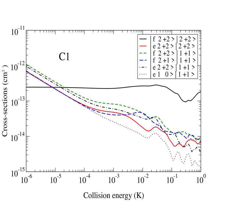
Figure 12: Dominant partial cross sections for OH$(\epsilon=f,f_{d}=2,m_{f_{d}}=2)$ + Rb$(f_{a}=2,m_{f_{a}}=2)$ incident channel (C1).

We first consider incident channel C1, with both collision partners initially in their maximally stretched states. Some of the main outcomes are shown in Fig 12. In the absence of an anisotropic interaction, and remembering that $M_{\mathcal{J}}=m_{f_{a}}+m_{f_{d}}+M_{L}$ is conserved, the sum of the spin projections $M_{F}=m_{f_{a}}+m_{f_{d}}$ would be conserved. Thus inelastic collisions would be impossible. This is because the projection of $m_{f_{d}}$ could not be lowered without raising $m_{f_{a}}$, but $m_{f_{a}}$ could not be raised further. However, the anisotropic PES in Rb-OH allows such changes quite readily.

There remains, however, a propensity for collisions with small values of $\Delta m_{f}$ to be more likely, as seen in Figure 13. Part (a) shows cross sections that change $m_{f_{d}}$ for OH without changing $m_{f_{a}}$ for Rb, while part (b) shows those that change $m_{f_{a}}$ without changing $m_{f_{d}}$. As noted above, Rb appears to be more reluctant to change its projection. In fact, since the potential is diagonal in the states of the nuclei, only consecutive values of $m_{f_{a}}$ are coupled in first order. On the other hand, first-order coupling exists between many different values of $m_{f_{d}}$. Finally, a decrease in the probability of processes with increasing $\Delta M_{F}$ can be related to the diminution of anisotropic terms in the potential when increasing the angular momentum transfer ($k$ in Eq. III.2).

Figure 13: Panel (a) ((b)): inelastic cross sections for $m_{f_{d}}$ ($m_{f_{a}}$) changing collisions. The higher the change, the lower the cross section. They correspond to OH$(\epsilon=f,f_{d}=2,m_{f_{d}}=2)$ + Rb$(f_{a}=2,m_{f_{a}}=2)$ incident channel (C1).

We now consider incident channel C2, OH$(\epsilon=e,f_{d}=1,m_{f_{d}}=1)$ + Rb$(f_{a}=1,m_{f_{a}}=-1)$. This is the lowest threshold in the absence of a field. Only three channels, degenerate with the initial channel, are possible outcomes at very low energies: $|\epsilon=e,1,{+1}\rangle|1,{-1}\rangle$ $|\epsilon=e,1,0\rangle|1,0\rangle$, and $|\epsilon=e,1,{-1}\rangle|1,{+1}\rangle$. Since these states have the same value of $M_{F}=m_{f_{d}}+m_{f_{a}}$ as the initial channel, the processes can occur by ordinary spin exchange with no centrifugal barrier. Partial cross sections for these three channels are shown in Figure 14 (a) over the entire energy range. Intriguingly, inelastic (state-changing) collisions seem to be somewhat suppressed relative to elastic scattering. Suppressed spin-exchange rates would presumably require delicate cancellation between singlet and triplet phase shifts Burke98 . That such a cancellation occurs in a highly multichannel process is somewhat unexpected. However, examining the matrix elements of the potential reveals that there is no direct coupling between the initial state $|\epsilon=e,1,{+1}\rangle|1,{-1}\rangle$ and final state $|\epsilon=e,1,{-1}\rangle|1,{+1}\rangle$. Transitions via potential couplings are therefore a second-order process requiring the mediation of other channels.

Many other exit channels are possible, once energy and angular momentum considerations permit them. Cross sections for several such processes are shown in Figure 14 (b). For example, the channels OH$(\epsilon=e,1,0)$ + Rb$(1,+1)$ and OH$(\epsilon=e,1,0)$ + Rb$(1,-1)$ are not connected to the initial channel by spin exchange, since $M_{F}$ changes by $-1$. In this case, angular momentum shunts from the molecule into the partial-wave degree of freedom, necessitating an $L=1$ partial wave in the exit channel. Therefore, this process is suppressed for energies below the $p$-wave centrifugal barrier, whose height is 1.6 mK.

Figure 14: Some partial cross sections for C2 incident channel: OH$(\epsilon=e,f_{d}=1,m_{f_{d}}=1)$ + Rb$(f_{a}=1,m_{f_{a}}=-1)$. On panel (a) elastic cross section together with partial cross sections for two degenerate processes with the initial channel, opened at zero collision energy, are shown. The processes shown on panel (b) are also degenerate but closed by the centrifugal barrier at zero collision energy.

We conclude this subsection by stressing the vital importance of including the hyperfine structure in these calculations. Figure 15 shows partial cross sections for incident channel C1 scattering into pairs of channels which differ only in the small hyperfine splitting of OH ($\approx 3$ mK). In one example (black and red solid curves), the parity of OH changes from $f$ to $e$, leading to the final channels OH$(\epsilon=e,f_{d}=1,2,m_{f_{d}}=0)$ + Rb$(f_{a}=2,m_{f_{a}}=0)$. These channels, distinguished only by their hyperfine quantum number $f_{d}$, are almost identical at high energies, but quite different at low energies. As a second example, consider the final channels OH$(\epsilon=f,f_{d}=1,2,m_{f_{d}}=0)$ + Rb$(f_{a}=2,m_{f_{a}}=+2)$, (green and orange dashed), which preserve the initial parity. The process with $f_{d}=1$ is exothermic, while the one with $f_{d}=2$ requires the opening of the partial wave threshold. Only after both channels are open, at higher energies, do the cross sections become almost identical.

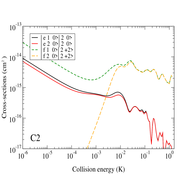
Figure 15: Partial cross sections for two pairs of processes corresponding to incident channel C1 (OH$(\epsilon=f,f_{d}=2,m_{f_{d}}=2)$ + Rb$(f_{a}=2,m_{f_{a}}=2)$) and final channels differing only in the $f_{d}$ quantum number. Their values converge at high kinetic energies but are very different in the cold regime.

IV.3 The harpooning process

We have not yet fully incorporated the ion-pair channel in our calculations, but it is instructive to assess its influence. In the harpooning model it is usually understood that, if the electron transfer takes place at long range, large collision cross sections result Ber . However, for Rb-OH the crossing point $R_{0}\approx 6$ Å gives a geometric cross section of only $\sigma=4\pi R_{0}^{2}\approx 4.5\cdot 10^{-14}$ cm². This is substantially smaller than the quantum-mechanical cross sections we have estimated. Thus while harpooning may enhance cross sections substantially at thermal energies, it is likely to have less overall influence in cold collisions.

The inelastic results above place cross sections near the semiclassical Langevin upper limit. The harpooning mechanism is unlikely to increase their magnitude, but could change their details. For example, it might be expected that the harpooning mechanism would distribute the total probability more evenly among the different spin orientations.

We have explored the influence of the harpooning mechanism in a reduced calculation where the hyperfine structure is neglected. This makes the calculation tractable even with the ion-pair channel included. The resulting elastic and total inelastic cross sections, for incident channel OH$(\epsilon=f,j=3/2,m=3/2)$ + Rb$(s_{a}=1/2,m_{s_{a}}=1/2)$ (maximally stretched in the absence of nuclear degrees of freedom) are shown in Figure 16. They are compared to the results obtained without the ion-pair channels. In the semiclassical region, $E>1$ mK, the general order of magnitude of the cross sections is preserved, although the detailed features are not. In the Wigner regime, by contrast, including the ion-pair channel makes a quite significant change, because completely different phase shifts are generated in low-lying partial waves. We stress again, however, that we do not expect this or any model to have predictive power for the values of low-energy cross sections until the ambiguities in absolute scattering lengths are resolved by experiments.

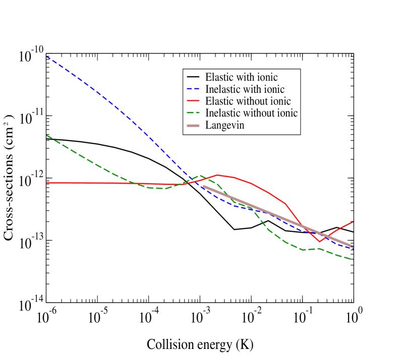
Figure 16: Effect of the inclusion of ion-pair channels in a reduced (neglecting hyperfine structure) calculation. Langevin cross section is also shown for comparison.

V Conclusions and prospects

Based on the results above, we can draw several general conclusions concerning both the feasibility of observing Rb-OH collisions experimentally in a beam experiment and the possibility of sympathetic cooling of OH using ultracold Rb.

We can assert with some confidence that Rb-OH cross sections at energies of tens of mK, typical of Stark decelerators, will be on the order of $10^{-13}\ \rm{cm}^{2}$. This is probably large enough to make the collisions observable. In round numbers, consider a Rb MOT with density $n_{\rm Rb}=10^{10}$ cm^-3, and an OH packet emerging from a Stark decelerator at 10 m/s, with density $n_{\rm OH}=10^{7}$ cm^-3. Further assume that the Rb is stored in an elongated MOT that allows an interaction distance of 1 cm as the OH passes through. In this case, a cross section $\sigma=10^{-13}$ cm² implies that approximately $10^{-3}$ of the OH molecules are scattered out of the packet. This quantity, while small, should be observable in repeated shots of the experiment Yun .

As for sympathetic cooling OH using cold Rb, it seems unlikely that this will be possible for species in their stretched states as in channel C1. The inelastic rates are almost always comparable to, or greater than, the elastic rates. The situation becomes even worse as the temperature drops and cross sections for exoergic processes diverge. Every collision event might serve to thermalize the OH gas, but is equally likely to remove the molecule from the trap altogether, or contribute to heating the gas.

For collision partners in the low-energy states of incident channel C2, the situation is not as bleak, at least in the low-energy limit, since inelastic cross sections do not diverge and may be fairly small. However, we have focused on the weak-magnetic-field seeking state of OH, which will not be the lowest-energy state in a magnetic field. Thus exoergic processes again appear, and inelastic rates will again become unacceptably large. Under these circumstances, rather than “sympathetic cooling,” the gas would exhibit “simply pathetic cooling.”

From these considerations, it seems that the only way to guarantee inelastic rates sufficiently low to afford sympathetic cooling would be to remove all exoergic inelastic channels altogether. Thus both species, atom and molecule, should be trapped in their absolute ground states, using optical or microwave dipole traps Mille or possibly an alternating current trap actrap . Sympathetic cooling would then be forced due to the absence of any possible outcome other than elastic and endoergic processes. The latter might produce a certain population of hyperfine-excited OH molecules, which could then give up their internal energy again and contribute towards heating. However, the molecules are far more likely to collide with atoms than with other molecules, so that this energy would eventually be carried away as the Rb is cooled.

Further aspects of the Rb-OH collision problem need further work. Foremost among these is the possibility that inelastic rates could be reduced or controlled by applying electric and/or magnetic fields. This may result partly from the simple act of moving Feshbach resonances to different energies, or from altering the effective coupling between incident and final channels, as has been hinted at previously Tick ; Krems . In addition, the influence of the ion-pair channel may be significant. There is the possibility, for example, that the highly polar RbOH molecule might be produced by absorption followed by either spontaneous or stimulated emission 9 . Finally, new phenomena are possible, such as analogues of the field-linked states that have been predicted in dipole-dipole collisions 31a ; 31b .

Appendix 1

As described above, we encountered difficulties with non-degeneracies between the ${}^{1}A^{\prime}$ and ${}^{1}A^{\prime\prime}$ components of the ${}^{1}\Pi$ state at linear geometries. These could have been avoided by carrying out the linear calculations in $C_{2v}$ rather than $C_{s}$ symmetry, but $C_{s}$ symmetry was essential to avoid discontinuities at $\theta=0$ and $180^{\circ}$.

To understand the non-degeneracies it is essential to understand the procedure used to generate the basis set used in the CISD calculation.

1. The molecular orbital basis set is partitioned into internal and external sets, and the internal orbitals are in turn partitioned into closed and active sets.

2. A reference space is generated, including all possible arrangements of the $N$ available electrons among the active orbitals that give states of the specified symmetry and spin multiplicity. The closed orbitals are doubly occupied in all reference configurations.

3. A set of $(N$–2)-electron states is generated by all possible 2-electron annihilations from the reference states (with no symmetry constraints). Some of the closed orbitals may be designated as core orbitals, in which case annihilations from them are not included.

4. A set of $(N$–1)-electron states is generated by all possible 1-electron additions to internal orbitals of the $(N$–2)-electron states (with no symmetry constraints).

5. The final CI basis includes states of 3 different classes:

   • Internal states are generated by all possible 1-electron additions to the $(N$–1)-electron states, with the extra electron in an internal orbital, that give states of the specified symmetry and spin multiplicity;

   • Singly external states are generated by all possible 1-electron additions to the $(N$–1)-electron states, with the extra electron in an external orbital, that give states of the specified symmetry and spin multiplicity;

   • Internally contracted doubly external states are generated by 2-electron excitations into the external space from a reference function obtained by solving a small CI problem in the reference space.

The non-degeneracies between the ${}^{1}A^{\prime}$ and ${}^{1}A^{\prime\prime}$ components of the ${}^{1}\Pi$ state arise from two different sources.

First, there is a part of the non-degeneracy due to the internal and singly external configurations. At linear geometries there are both $\Sigma$-type and $\Pi$-type reference configurations. Both types are included for $A^{\prime}$ symmetry, but only the $\Pi$-type reference configurations are included for $A^{\prime\prime}$ symmetry. In the $A^{\prime}$ calculation, therefore, there are additional $\Pi$-type internal and singly external configurations that arise from $\Sigma$-type reference configurations. This effect could in principle be suppressed in MOLPRO by including reference configurations of both symmetries in both calculations at all geometries, but this was prohibitively expensive in computer time. In addition, as described below, it is responsible for only about 20% of the total non-degeneracy.

Secondly, there is a part of the non-degeneracy due to the (contracted) doubly external configurations. It must be remembered that we wish to transform the $1A^{\prime}$ and $2A^{\prime}$ singlet states into a diabatic representation. To do this meaningfully, we need them to be calculated using identical basis sets. If we do the MRCI calculations separately, this is not true: even if the reference space is the same, each state produces a different set of internally contracted doubly external states. It is thus necessary to calculate the two ${}^{1}A^{\prime}$ states in the same MRCI block, so that the basis set contains both sets of contracted functions. However, this results in a larger and more flexible basis set of contracted doubly external functions than is generated in the ${}^{1}A^{\prime\prime}$ case.

It is helpful to document the magnitude of the non-degeneracies in various possible calculations. For RbOH at $\theta=0$ and $R=12$ Å:

• If calculations are carried out in $C_{2v}$ symmetry, the ion-pair and covalent states have different symmetry and the non-degeneracy is not present;

• For $C_{s}$ symmetry with the two ${}^{1}A^{\prime}$ states calculated in a single MRCI block, both sources of non-degeneracy are present and the non-degeneracy is $22.78\,\mu E_{h}$;

• For $C_{s}$ symmetry with the two ${}^{1}A^{\prime}$ states calculated in separate MRCI blocks, only the first source of non-degeneracy is present and the non-degeneracy is $4.08\,\mu E_{h}$;

• For $C_{s}$ symmetry with the two ${}^{1}A^{\prime}$ states calculated in a single MRCI block, but reference configurations of both symmetries included, only the second source of non-degeneracy is present and the non-degeneracy is $18.70\,\mu E_{h}$;

• For $C_{s}$ symmetry with the two ${}^{1}A^{\prime}$ states calculated in separate MRCI blocks, with reference configurations of both symmetries included, there is no non-degeneracy.

Appendix 2

The interaction potential does not involve the spins of the nuclei and is diagonal in the total electronic spin $S$. This makes it expedient to define two additional basis sets.

Basis set B2 is based on Hund’s case (b) quantum numbers for the molecule: the orbital angular momentum of the electron and the rotational angular momentum couple to form $n$, with $\lambda$ projection on the internuclear axis. $n$ coupled to the spin of the electron $s_{d}$ would give us $j$ for the diatomic fragment, as in basis set B1. Instead, in B2 we couple $s_{d}$ with $s_{a}$ to obtain the total spin of the electrons, described by kets $|SM_{S}\rangle$. However, we leave aside the states of the nuclei, which are represented by $|i_{a}m_{i_{a}}\rangle|i_{d}m_{i_{d}}\rangle$, with $m_{i_{a}}$ and $m_{i_{d}}$ being the projections of the nuclear spin of the atom and diatom in the laboratory frame. Basis set B2w is then given by

$$|B2w\rangle=|(s_{d}s_{a})SM_{S}\rangle|nm_{n}\lambda\rangle|i_{d}m_{i_{d}}\rangle|i_{a}m_{i_{a}}\rangle|LM_{L}\rangle,$$ (66)

where $|nm_{n}\lambda\rangle$ represents $\sqrt{\frac{2n+1}{8\pi^{2}}}D_{m_{n}\lambda}^{n*}(\alpha,\beta,\gamma)$. The parity operator $E^{*}$ acts on these states as follows:

$$E^{*}|(s_{d}s_{a})SM_{S}\rangle|nm_{n}\lambda\rangle|i_{d}m_{i_{d}}\rangle|i_{a}m_{i_{a}}\rangle|LM_{L}\rangle=$$

$$(-1)^{n+L}|(s_{d}s_{a})SM_{S}\rangle|nm_{n}-\lambda\rangle|i_{d}m_{i_{d}}\rangle|i_{a}m_{i_{a}}\rangle|LM_{L}\rangle,$$

which allows us to construct combinations of define parity,

$$|B2p\rangle=|(s_{d}s_{a})SM_{S}\rangle|nm_{n}\bar{\lambda}\epsilon\rangle|i_{d}m_{i_{d}}\rangle|i_{a}m_{i_{a}}\rangle|LM_{L}\rangle.$$ (68)

The third basis set, B3, is intermediate between B1 and B2. Here the molecule is again labeled by quantum numbers corresponding to a Hund’s case (a) molecule, as in B1,

$$|B3w\rangle=|s_{d}\sigma\rangle|\lambda\rangle|jm\omega\rangle|i_{d}m_{i_{d}}\rangle|s_{a}m_{s_{a}}\rangle|i_{a}m_{i_{a}}\rangle|LM_{L}\rangle.$$ (69)

However, the part describing the OH fragment is taken as $|jm\omega\rangle|\lambda\rangle|s_{d}\sigma\rangle$, that is, with signed values of $\lambda$, $\sigma$, and $\omega$. In this case, the parity operator $E^{*}$ acts as follows,

$$E^{*}|s_{d}\sigma\rangle|\lambda\rangle|jm\omega\rangle|i_{d}m_{i_{d}}\rangle|s_{a}m_{s_{a}}\rangle|i_{a}m_{i_{a}}\rangle|LM_{L}\rangle$$

$$=(-1)^{j-s_{d}+L}$$

$$\times|s_{d}-\sigma\rangle|-\lambda\rangle|jm-\omega\rangle|i_{d}m_{i_{d}}\rangle|s_{a}m_{s_{a}}\rangle|i_{a}m_{i_{a}}\rangle|LM_{L}\rangle,$$ (70)

so that we can again build combinations of defined parity,

$$|B3p\rangle=|s_{d}\bar{\lambda}\bar{\omega}\epsilon jm\rangle|i_{d}m_{i_{d}}\rangle|s_{a}m_{s_{a}}\rangle|i_{a}m_{i_{a}}\rangle|LM_{L}\rangle.$$ (71)

The change from B2w to B3w, leaving aside the partial wave and nuclear spin states, is given by

$$|s_{d}\sigma\rangle |\lambda\rangle|jm\omega\rangle|s_{a}m_{s_{a}}\rangle$$

$$= \sum_{m_{s_{d}}}\sum_{n}\sum_{S}\sum_{M_{S}}\left(\begin{array}[]{ccc}s_{d}&s_{a}&S\\ m_{s_{d}}&m_{s_{a}}&-M_{S}\end{array}\right)\left(\begin{array}[]{ccc}s_{d}&n&j\\ m_{s_{d}}&m_{n}&-m\end{array}\right)\left(\begin{array}[]{ccc}s_{d}&n&j\\ -\sigma&-\lambda&\omega\end{array}\right)$$

$$\times (-1)^{(m-\omega+s_{d}-s_{a}+M_{S})}|nm_{n}\lambda\rangle|(s_{d}s_{a})SM_{S}\rangle.$$

References

- (1) J. J. Hudson, B. E. Sauer, M. R. Tarbutt, and E. A. Hinds, Phys. Rev. Lett. 89, 023003 (2002).
- (2) L. Santos, G. V. Shlyapnikov, P. Zoller, and M. Lewenstein, Phys. Rev. Lett. 85, 1791 (2000); Phys. Rev. Lett. 88, 139904(E) (2002).
- (3) K. Goral, L. Santos, and M. Lewenstein, Phys. Rev. Lett. 88, 170406 (2002).
- (4) B. Damski, L. Santos, E. Tiemann, M. Lewenstein, S. Kotochigova, P. Julienne, and P. Zoller, Phys. Rev. Lett. 90, 110401 (2003).
- (5) M. A. Baranov, M. S. Marenko, V. S. Rychkov, and G. V. Shlyapnikov, Phys. Rev. A 66, 013606 (2002).
- (6) N. Balakrishnan and A. Dalgarno, Chem. Phys. Lett. 341, 652 (2001).
- (7) E. Bodo and F. A. Gianturco, Eur. Phys. J. D 31, 423 (2004).
- (8) P. F. Weck and N. Balakrishnan, Eur. Phys. J. D 31, 417 (2004).
- (9) E. R. Hudson, H. J. Lewandowski, B. C. Sawyer, and J. Ye, physics/0601054.
- (10) P. Soldán, M. T. Cvitaš, J. M. Hutson, and C. S. Adams (Eds.), Interactions of Cold Atoms and Molecules (CCP6, Daresbury, 2002).
- (11) Ultracold Polar Molecules: Formation and Collisions. Special issue of Eur. Phys. J. D 31, No. 2 (2004).
- (12) J. M. Hutson and P. Soldán, Int. Rev. Phys. Chem. 25, xxx (2006) (in press for October 2006: update in proof).
- (13) R. V. Krems, Int. Rev. Phys. Chem. 24, 9 9 (2005).
- (14) P. F. Weck and N. Balakrishnan, Int. Rev. Phys. Chem. 25, 283 (2006).
- (15) E. Bodo and F. A. Gianturco, Int. Rev. Phys. Chem. 25, 313 (2006).
- (16) H. L. Bethlem, F. M. H. Crompvoets, R. T. Jongma, S. Y. T. van de Meerakker, and G. Meijer, Phys. Rev. A 65, 053416 (2002).
- (17) H. L. Bethlem and G. Meijer, Int. Rev. Phys. Chem. 22, 73 (2003).
- (18) J. R. Bochinski, E. R. Hudson, H. J. Lewandowski, and J. Ye, Phys. Rev. A 70, 043410 (2004).
- (19) R. deCarvalho, J. M. Doyle, B. Friedrich, T. Guillet, J. Kim, D. Patterson, and J. D. Weinstein, Eur. Phys. J. D 7, 289 (1999).
- (20) D. J. Larson, J. C. Bergquist, J. J. Bollinger, W. M. Itano, and D. J. Wineland, Phys. Rev. Lett. 57, 70 (1986).
- (21) B. Roth, C. Zhang, D. Offenberg, A. Wilson, A. Ostendorf, and S. Schiller, unpublished work.
- (22) G. Modugno, G. Ferrari, G. Roati, R. J. Brecha, A. Simoni, and M. Inguscio, Science 294, 1320 (2001).
- (23) L. González-Sánchez, E. Bodo, and F. A. Gianturco, Phys. Rev. A 73, 022703 (2006).
- (24) N. Balakrisnan, G. C. Groenenboom, R. V. Krems, and A. Dalgarno, J. Chem. Phys. 118, 7386 (2003).
- (25) H. Cybulski, R. V. Krems, H. R. Sadeghpour, A. Dalgarno, J. Kłos, G. C. Groenenboom, A. van der Avoird, D. Zgid, and G. Chałasinski, J. Chem. Phys. 122, 094370 (2005).
- (26) R. C. Forrey, V. Kharchenko, N. Balakrishnan, and A. Dalgarno, Phys. Rev. A 59, 2146 (1998).
- (27) J. L. Bohn, Phys. Rev. A 61, 040702(R) (2000); ibid., 62, 032701 (2000).
- (28) T. Stoecklin, A. Voronin, and J. C. Rayez, Phys. Rev. A 66, 042703 (2002).
- (29) P. Soldán, M. T. Cvitaš, J. M. Hutson, P. Honvault, and J.-M. Launay, Phys. Rev. Lett. 89, 153201 (2002).
- (30) M. T. Cvitaš, P. Soldán, J. M. Hutson, P. Honvault, and J.-M. Launay, Phys. Rev. Lett. 94, 033201 (2005).
- (31) M. T. Cvitaš, P. Soldán, J. M. Hutson, P. Honvault, and J.-M. Launay, Phys. Rev. Lett. 94, 200402 (2005).
- (32) G. Quéméner, P. Honvault, J.-M. Launay, P. Soldán, D. E. Potter and J. M. Hutson, Phys. Rev. A 71, 032722 (2005).
- (33) M. Lara, J. L. Bohn, D. E. Potter, P. Soldán, and J. M. Hutson, Phys. Rev. Lett. (submitted).
- (34) S. Y. T. van de Meerakker, P. H. M. Smeets, N. Vanhaecke, R. T. Jongma, and G. Meijer, Phys. Rev. Lett. 94, 023004 (2005).
- (35) T.-S. Ho and H. Rabitz, J. Chem. Phys. 104, 2584 (1996).
- (36) R. D. Levine and R. B. Bernstein, Molecular Reaction Dynamics and Chemical Reactivity (Oxford University Press, 1987), p. 134.
- (37) P. Soldán and J. M. Hutson, Phys. Rev. Lett. 92, 163202 (2004).
- (38) H.-J. Werner, P. J. Knowles, R. Lindh, M. Schütz et al., MOLPRO quantum chemistry package, version 2002.6 (2002). For more information see http://www.molpro.net/
- (39) T. Leininger, A. Nicklass, W. Kuchle, H. Stoll, M. Dolg, and A. Bergner, Chem. Phys. Lett. 255, 274 (1996).
- (40) P. Soldán, M. T. Cvitaš, and J. M. Hutson, Phys. Rev. A 67, 054702 (2003).
- (41) T. H. Dunning, Jr., J. Chem. Phys. 90, 1007 (1989).
- (42) M. Abramowitz and I. A. Stegun (Eds.), Handbook of Mathematical Functions, 9th printing (Dover, New York, 1972), p. 888.
- (43) H.-J. Werner and P. J. Knowles, J. Chem. Phys. 89, 5803 (1988).
- (44) J. A. Pople and H. C. Longuet-Higgins, Mol. Phys. 1, 372 (1958).
- (45) E. P. F. Lee and T. G. Wright, J. Phys. Chem. A 107, 5233 (2003).
- (46) A. Degli Esposti and H.-J. Werner, J. Chem. Phys. 93, 3351 (1990).
- (47) M.-L. Dubernet and J. M. Hutson, J. Chem. Phys. 99, 7477 (1993).
- (48) H.-S. Lee, A. B. McCoy, R. R. Toczłowski, and S. M. Cybulski, J. Chem. Phys. 113, 5736 (2000).
- (49) S. F. Boys and F. Bernardi, Mol. Phys. 19, 553 (1970).
- (50) M. Meuwly and J. M. Hutson, J. Chem. Phys. 110, 8338 (1999).
- (51) P. Soldán, E. P. F. Lee, and T. G. Wright, J. Chem. Phys. 116, 2395 (2002). There is a typographical error in Eq. 4 of this paper: the “” sign should be “+” in this equation.
- (52) T.-S. Ho and H. Rabitz, J. Chem. Phys. 113, 3960 (2000).
- (53) P. Soldán and J. M. Hutson, J. Chem. Phys. 112, 4415 (2000).
- (54) T. Hollebeek, T.-S. Ho, and H. Rabitz, Annu. Rev. Phys. Chem. 50, 537 (1999).
- (55) D. M. Brink and G. R. Satchler, Angular Momentum, 3rd ed. (Oxford University Press, 1993).
- (56) J. A. Coxon, Can. J. Phys. 58, 933 (1980).
- (57) E. Arimondo, M. Inguscio, and P. Violino, Rev. Mod. Phys. 49, 31 (1977).
- (58) I. Johansson, Ark. Fys. 20, 135 (1961).
- (59) B. R. Johnson, J. Comput. Phys. 14, 445 (1973).
- (60) N. F. Mott and H. S. W. Massey, The Theory of Atomic Collisions, 3rd ed. (Clarendon Press, Oxford, 1965).
- (61) E. S. Chang and U. Fano, Phys. Rev. A 6, 173 (1972).
- (62) J. P. Burke, C. H. Greene, and J. L. Bohn, Phys. Rev. Lett. 81, 3355 (1998).
- (63) B. Gao, E. Tiesinga, C. J. Williams, and P. S. Julienne, Phys. Rev. A 72, 042719 (2005).
- (64) R. D. Levine and R. B. Bernstein, Molecular Reaction Dynamics and Chemical Reactivity (Oxford University Press, 1987).
- (65) J. Ye, private communication.
- (66) D. DeMille, D. R. Glenn, and J. Petricka, Eur. Phys. J. D 31, 375 (2004)
- (67) J. van Veldhoven, H. L. Bethlem, and G. Meijer, Phys. Rev. Lett. 94, 083001 (2005).
- (68) C. Ticknor and J. L. Bohn, Phys. Rev. A 71, 022709 (2005).
- (69) A. V. Avdeenkov, D. C. E. Bortolotti, and J. L. Bohn, Phys. Rev. A 69, 012710 (2004).
- (70) A. V. Avdeenkov and J. L. Bohn, Phys. Rev. Lett. 90, 043006 (2003).
- (71) S. Inouye, J. Goldwin, M. L. Olsen, C. Ticknor, J. L. Bohn, and D. S. Jin, Phys. Rev. Lett. 93, 183201 (2004).
- (72) J. M. Vogels, B. J. Verhaar, and R. H. Blok, Phys. Rev. A 57, 4049 (1998).
- (73) J. P. Burke, J. L. Bohn, B. D. Esry, and C. H. Greene, Phys. Rev. A 55, R2511 (1996).
- (74) H. J. Metcalf and P. van der Straten, Laser Cooling and Trapping (Springer, New York, 1999).