Reconstructing the impulse response of a diffusive medium with the Kramers-Kronig relations

Abstract

The Kramers-Kronig (KK) algorithm, useful for retrieving the phase of a spectrum based on the known spectral amplitude, is applied to reconstruct the impulse response of a diffusive medium. It is demonstrated by a simulation of a 1D scattering medium with realistic parameters that its impulse response can be generated from the KK method with high accuracy.

]

I introduction

Recently there has been a growing interest in light propagation in diffusive or turbid media [1]. This can be attributed to several areas of application-driven research. Diffusive media are ubiquitous in our environment, and imaging through them is always a challenge. Clouds, mist, fog, dust and smoke decrease the visibility on land while surface waves and turbid water reduce visibility at sea. In the medical field, the main obstacle that a physician encounters while trying to diagnose internal organs is the diffusivity rather than the absorption of the biological tissues. As a consequence, many methods were developed to image through and to investigate diffusive media [1].

One of the most intuitive methods to investigate a diffusive medium is to measure its’ impulse response by a fast detector [2, 3, 4, 5, 6], since, in principle, the impulse response carries all the optical information of any linear medium. In practice, fast detectors measure the intensity of the impulse response. The ’first-light’ component of the impulse response carries the ballistic information of the medium. This information can be used in the reconstruction of the ballistic image of the diffusive medium. Obviously, since the number of ballistic photons is extremely small, the image can be partially reconstructed by the quasi-ballistic (or ”snake”) photons, which would impair the spatial resolution of the image.

Assuming that the amount of detected quasi-ballistic photons is sufficient for the image reconstruction, in order to obtain high resolution images the detectors must be very fast to distinguish between the (quasi) ballistic and the diffusive photons. As a consequence such an imaging technique requires complicated and expensive equipment.

This is one of the main motivations for developing spectral techniques [7, 8, 9, 10], i.e., techniques which work in the spectral domain instead of the temporal one [4, 5, 6]. In one of these techniques the spectral response of the medium $H\left(\omega\right)=A\left(\omega\right)\exp\left[{i\varphi\left(\omega\right)}\right]$ is measured for each wavelength in a wide spectral range [11, 12, 13]. While an amplitude $A\left(\omega\right)$ measurement is a relatively simple task (and fast, since it does not require long averaging), a phase $\varphi\left(\omega\right)$ measurement is more complicated since it usually requires interferometric processes that are inherently complicated and susceptible to fluctuations. Therefore, phase measurements are of limited value when the medium varies in time. However, if the phase is reconstructed from the amplitude measurement and the process is sufficiently fast, the temporal impulse response can be easily generated even for a varying medium by a simple inverse Fourier transform. Since in most cases the diffusive medium can be regarded as linear (and hopefully time-invariant) system the Kramers-Kronig (KK) method [14, 15] can be used to derive the phase from the amplitude measurement.

Nevertheless, the KK method has several drawbacks. Firstly, in order to derive the phase one needs the amplitude over the entire spectrum (from zero to infinity), while experiments can produce amplitude measurements for only a finite range of frequencies. As a consequence, any evaluation of phases with the KK method is always an approximation (see, for example, ref.[16]). Some methods were developed to improve these approximations (by improving the convergence of the integrals) such as the singly and multiply subtractive KK relations ([17] and [18] respectively).

A more complicated problem arises from the logarithm function, which diverges whenever the spectral response of the medium $H\left(\omega\right)$ vanishes. As a consequence the full KK relation is [19]

$$\varphi_{KK}(\omega)=-\frac{\omega}{\pi}P\int_{0}^{\infty}d\omega^{\prime}\frac{\ln|H(\omega^{\prime})|}{\omega^{\prime 2}-\omega^{2}}+\sum_{j}\arg\left(\frac{\omega-\omega_{j}}{\omega-\omega^{*}_{j}}\right)$$ (1)

where the $P$ denotes Cauchy’s principal value. The first term on the right is the ordinary KK relation, while the second one is the Blaschke term, which takes account all of the zeros $\omega_{j}$ of $H\left(\omega\right)$.

The problem with the zeros of $H\left(\omega\right)$ is more fundamental since while the first mentioned problem can be mitigated, at least in principle, by measuring the amplitude for a larger spectral range, the zeros of $H\left(\omega\right)$ cannot in general be deduced from the amplitude measurements alone. This problem is confronted mainly in reflection measurements, where $H\left(\omega\right)$ may vanish at certain complex frequencies (for a discussion on this subject see refs. [20] and [21]). However, a diffusive medium in the transmission configuration is a good candidate for the implementation of the KK method in the following case.

In any diffusive medium the diffusion coefficient of the medium $D$ and its size $L$ determines the smallest frequency scale $\delta\omega\sim D/L^{2}$, which is related to its reciprocal parameter $t_{D}\sim L^{2}/D$ – the mean time a photon dwells in the diffusive medium . If the measured spectral range $\Delta\omega\equiv\omega_{\max}-\omega_{\min}$ is considerably larger than $\delta\omega$ then the main features of the impulse response can be retrieved from the KK relations. Moreover, we will demonstrate that in this regime it is possible to evaluate the amplitude $\left|{H\left(\omega\right)}\right|$ beyond the spectral range (i.e., $\omega<\omega_{\min}$ and $\omega>\omega_{\max})$ by a certain average over its values inside $\omega_{\min}<\omega<\omega_{\max}$. In what follows we will revert to wavenumbers instead of frequencies, but the transition between the two is trivial.

In most previous works the desired parameter was the refractive index of a medium, so that the KK method was mostly implemented for cases where the attenuation was caused by absorption rather than by scattering. As a result, using the KK method as a tool to measure the impulse response of a diffusive medium was not common. Recently, we demonstrated [12] that the KK method, even in its simplest and most naive form can be used to reconstruct the impulse response of a Fabry-Perot interferometer, whose response is governed solely by scattering. It was shown that with relatively simple equipment its’ impulse response can be evaluated with very high temporal resolution (less than 200fs).

In this paper we demonstrate by a numerical simulation that the KK method can be useful in determining the phases of the transfer function of a diffusive medium. It is also shown that the calculated spectral response can be used in reconstructing the medium’s impulse response with high accuracy.

II The model

We investigate a 1D homogenous medium with $N$ small scatterers, each having a different refractive index and width, randomly distributed in the medium. For simplicity it is assumed that the width of each scatterer $l_{j}$ is considerably smaller than the beam’s wavelength $\lambda$ (i.e., $l_{j}<<\lambda$ for every $j)$, however, this is not a restrictive assumption since a diffusive medium, whose dimensions are considerably larger than the medium’s diffusion length is characterized, almost by definition, only by a median value for the scattering coefficient (i.e., as long as the set of scattering coefficients are similar the fine structure of each scatterer is not important; similarly, the exact locations of the scatterers have a negligible effect on the diffusion coefficient).

For simplicity we ignore polarization effects, and thus the 1D stationary-state wave equation has the form

$$\frac{\partial^{2}}{\partial x^{2}}\psi^{2}+\left({\frac{2\pi n\left(x\right)}{\lambda}}\right)^{2}\psi=0$$ (2)

where $\psi\left(x\right)$ is the electromagnetic field and $n\left(x\right)$ is the refractive index.

In general, the refractive index of a diffusive medium, modeled as a homogenous medium with multiple random scatterers, has the general form presented in fig.1. For simplicity, however, we choose to simulate the variations in the refractive index of the medium by delta functions, which corresponds to scatterers whose dimensions $l_{j}$ are considerably smaller than the beam’s wavelength $l_{j}<<\lambda$, consistent with our previous assumption. It should be stressed, that any small 1D scatterer (with respect to the wavelength) can be replaced for any practical reason with a delta function, the reason being that neither its width $l_{j}$ nor its strength $\delta n_{j}$ (the difference between its refraction index and the surrounding) appears separately in the scattering solutions, only their product $l_{j}\delta n_{j}$ does. Therefore, a small scatterer, whose width and strength are $l_{j}$ and $\delta n_{j}$ respectively can be replaced by a delta function whose prefactor is proportional to $l_{j}\delta n_{j}$ (see below for details).

FIG. 1.: Refractive index as a function of location for a diffusive medium

The square of the refraction index can be separated into homogenous ($n_{0}^{2})$ and varying ($2n_{0}\Delta n)$ parts

$$\frac{\partial^{2}}{\partial x^{2}}\psi^{2}+\left({\frac{2\pi}{\lambda}}\right)^{2}\left[{n_{0}^{2}+2n_{0}\Delta n\left(x\right)}\right]\psi=0$$ (3)

With the definition of the wavenumber $k\equiv 2\pi n_{0}/\lambda$ the wave equation can be written

$$\frac{\partial^{2}}{\partial x^{2}}\psi+k^{2}\left({1+2\frac{\Delta n\left(x\right)}{n_{0}}}\right)\psi=0,$$ (4)

where $2\Delta n\left(x\right)/n_{0}=\sum\limits_{j=1}^{N}{\alpha_{j}\delta\left({x-L_{j}}\right)}$, $N$ is the number of scatterers, $L_{j}=L_{j-1}+a_{j}=\sum\limits_{m=1}^{j}{a_{m}}$ is the position of the $j$th scatterer, i.e., $a_{j}$ are the distances between two adjacent scatterers, and

$$\alpha_{j}=2\frac{\delta n_{j}l_{j}}{n_{0}}$$ (5)

is the strength of the $j$th scatterer, where $\delta n_{j}$ and $l_{j}$ are the change in its refractive index and its size respectively.

Therefore, the wave equation for the diffusive medium reads

$$\frac{\partial^{2}}{\partial x^{2}}\psi+k^{2}\left[{1+\sum\limits_{j=1}^{N}{\alpha_{j}\delta\left({x-L_{j}}\right)}}\right]\psi=0\quad.$$ (6)

FIG. 2.: A schematic presentation of the diffusive medium. Each scatterer is presented in the model as a delta function change in the refractive index.

In the appendix we elaborate on the derivation of the medium’s spectral response $H\left(k\right)$ from eq.6. We then apply the KK method to a finite spectrum $k_{\min}\leq k\leq k_{\max}$ to determine the phase:

$$\varphi_{KK}\left(k\right)=-\frac{k}{\pi}P\int\limits_{k_{\min}}^{k_{\max}}{dk^{\prime}\frac{\ln\left|{H\left({k^{\prime}}\right)}\right|}{k^{\prime 2}-k^{2}}}.$$ (7)

which is then substituted into:

$$H_{KK}\left(k\right)=\left|{H\left(k\right)}\right|\exp\left[{i\varphi_{KK}\left(k\right)}\right]$$ (8)

to evaluate the medium’s spectral response. If we keep $\Delta k\equiv k_{\max}-k_{\min}>>Dn/\left({cL^{2}}\right)$ (where $n$ is the refractive index of the medium) then most of the features of the impulse response can be derived. Moreover, in this regime, approximation (7) can be improved by noticing that the mean value of $\ln\left|{H\left(k\right)}\right|$ does not change much beyond the measured region $k_{\min}\leq k\leq k_{\max}$ (at least in its spectral vicinity). Therefore, the boundaries of the integral (7) can be taken as 0 and $\infty$ while $\ln\left|{H\left(k\right)}\right|$ for $0<k<k_{\max}$and $k_{\max}<k<\infty$ is replaced with its average value, i.e.,

$$\begin{array}[]{l}\varphi_{KK}\left(k\right)=-\frac{k}{\pi}P\int\limits_{k_{\min}}^{k_{\max}}{dk^{\prime}\frac{\ln\left|{H\left({k^{\prime}}\right)}\right|}{k^{\prime 2}-k^{2}}}-\\ \frac{k}{\pi}\left\langle{\ln\left|{H\left(k\right)}\right|}\right\rangle\left[{\int\limits_{0}^{k_{\min}}{dk^{\prime}\frac{1}{k^{\prime 2}-k^{2}}+\int\limits_{k_{\max}}^{\infty}{dk^{\prime}\frac{1}{k^{\prime 2}-k^{2}}}}}\right]\\ \end{array}$$ (9)

where $\left\langle{\ln\left|{H\left(k\right)}\right|}\right\rangle\equiv\left({k_{\max}-k_{\min}}\right)^{-1}\int_{k_{\min}}^{k_{\max}}{dk^{\prime}}\ln\left|{H\left({k^{\prime}}\right)}\right|$ is the mean value of $\ln\left|{H\left(k\right)}\right|$ in the measured region.

It should be noted that in cases where the KK method is used to derive the refractive index (as is the case in negligibly scattering media) the variations in $\ln\left|{H\left(k\right)}\right|$ are of the same scale as the spectral range $\Delta k$, i.e., $d\ln\left|{H\left(k\right)}\right|/dk\sim\Delta k^{-1}$. Therefore, in these cases analytical continuation and extrapolations are used to approximate $\ln\left|{H\left(k\right)}\right|$ beyond the measured region [22]. In the scattering medium case the situation is considerably different, namely $d\ln\left|{H\left(k\right)}\right|/dk>>\Delta k^{-1}$, and therefore extrapolations has little value. On the other hand the spectral variations are so strong that they rapidly converge to the average value.

By solving the integrals one obtains an evaluation of the phases from the amplitude measurements

$$\varphi_{KK}\left(k\right)=-\frac{k}{\pi}P\int\limits_{k_{\min}}^{k_{\max}}{dk^{\prime}\frac{\ln\left|{H\left({k^{\prime}}\right)}\right|}{k^{\prime 2}-k^{2}}}+\Delta\varphi_{KK}\left(k\right)$$ (10)

where

$$\Delta\varphi_{KK}\left(k\right)\equiv-\frac{1}{2\pi}\left\langle{\ln\left|{H\left(k\right)}\right|}\right\rangle\ln\left({\frac{k-k_{\min}}{k+k_{\min}}\cdot\frac{k_{\max}+k}{k_{\max}-k}}\right)$$ (11)

is a correction term.

This phase is then substituted into eq. (8) to reconstruct the full transfer function.

If the spectrum of the input signal is a rectangular function in the spectral domain $k_{\min}\leq k\leq k_{\max}$ (and therefore the field is proportional to $E_{in}\left(t\right)\propto\exp\left({i\bar{k}ct}\right){\mathrm{sinc}}\left({\Delta kct/2}\right)$, where $\Delta k\equiv k_{\max}-k_{\min}$ and $\bar{k}\equiv\left({k_{\max}+k_{\min}}\right)/2)$ the exact impulse response, which will be measured at the end of the medium, i.e., at $x>L_{N}$, is

$$I\left(t\right)=\left|{\int\limits_{k_{\min}}^{k_{\max}}{dk^{\prime}H\left({k^{\prime}}\right)\exp\left({ik^{\prime}ct}\right)dk^{\prime}}}\right|^{2}$$ (12)

while the KK reconstruction, which is based only on the amplitude (or intensity) measurements, predicts

$$I_{KK}\left(t\right)=\left|{\int\limits_{k_{\min}}^{k_{\max}}{dk^{\prime}H_{KK}\left({k^{\prime}}\right)\exp\left({ik^{\prime}ct}\right)dk^{\prime}}}\right|^{2}.$$ (13)

We will demonstrate by a simulation that in a realistic case the latter expression is a very good approximation to the former.

III Simulation

For simplicity we choose air as the homogenous medium, i.e., $n_{0}=1$ (however, the results can easily be scaled to any dielectric medium with an arbitrary $n_{0})$ with 150 small scatterers, where the distance between them is a random variable, distributed uniformly between 0 and $5\mu m$ (i.e., $0\leq a_{j}\leq 5\mu m)$. Similarly, the strength of each scatterer is also a uniform random number so that $0\leq\alpha_{j}\leq 0.03\mu m$ (this corresponds to glass particles having widths on the order of tens of nanometers).

FIG. 3.: The impulse response of the medium. The upper plot is the exact reconstruction, while the lower one is the KK reconstruction.

We assume that the incoming pulse that penetrates the medium has a rectangular spectral shape, i.e., $E_{in}\left(t\right)\propto\exp\left({i\bar{k}ct}\right){\mathrm{sinc}}\left({\Delta kct/2}\right)$, with $\bar{\omega}\equiv\bar{k}c=2\pi\times 750\mbox{THz}$ and $\Delta\omega\equiv\Delta kc=2\pi\times 300\mbox{THz}$.

Since $D\cong cl_{RW}/n$ where $l_{RW}\cong a/R$ ($a$ is the average distance between scatterers and $R$ is the mean reflection coefficient) is the random walk in the diffusion process, then the minimum spectral range required is $\delta k\cong a/RL^{2}=\left({NRL}\right)^{-1}$ (where $N$ is the total number of scatterers).

In this case the measured spectral range is six orders of magnitude larger than $\delta k$ i.e., $\delta k\cong 15m^{-1}<<6.3\times 10^{6}m^{-1}\cong\Delta k$.

In Fig.3 the reconstruction of the impulse responses of the exact solution $I\left(t\right)$ and the KK reconstruction $I_{KK}\left(t\right)$ are presented.

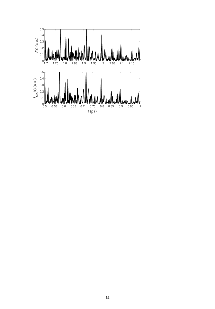
FIG. 4.: Zoom-in of fig.3

As can be seen, except for the delay between the two pulses, which is a direct consequence of the KK technique, the two signals are very similar. Evidently, they are not identical but the differences between them are quite small. In Fig.4 we reveal details of the temporal response and compare the two responses over a small temporal window, showing that the two are alike even on the microscopic level.

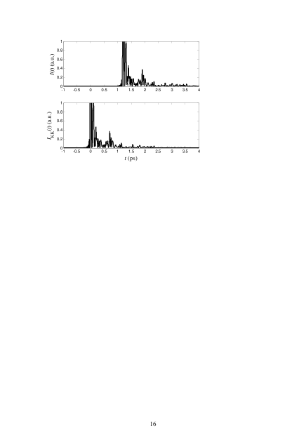
FIG. 5.: Same as Fig.3 but with a spectral width of $\Delta\omega=2\pi\times 30\mbox{THz}$.

If the spectrum of the incoming pulse is narrower, i.e., the incoming pulse is temporally broader, the spikes in the outgoing pulse are respectively wider. In Fig. 5 and 6 the impulse response of the same system is presented when the spectral width of the incoming pulse is ten times narrower (than in Figs. 3 and 4), that is, $\Delta\omega=2\pi\times 30\mbox{THz}$. As can be seen from these plots, the KK approximation is even better for the spectrally narrow pulse. Therefore, although the integration in the KK expressions covers a narrower region, and in principle should yield inferior results, since the spikes are temporally wider and therefore are less susceptible to dispersion deformation, the reconstruction is improved. The problem is, however, that as $\Delta k$ decreases and gets closer to $\delta k$ there is insufficient spectral information to reconstruct the complete impulse response and the error in the evaluation of macroscopic averages (such as the diffusion coefficient) increases.

FIG. 6.: Same as Fig.4 but with a spectral width of $\Delta\omega=2\pi\times 30\mbox{THz}$.

IV The effect of the correction term

To illustrate the importance of the correction term $\Delta\varphi_{KK}\left(k\right)$ in eq.8 we repeat the simulation for a bandwidth $\Delta\omega\equiv\Delta kc=2\pi\times 150\mbox{THz}$ with and without the CT.

In the upper panel of Fig.7 the reconstruction was made with the CT, and in the lower panel the CT was absent. There is a clear improvement in the upper panel.

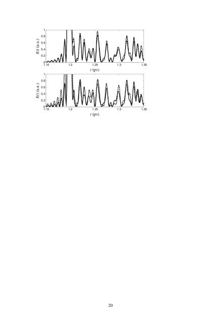
FIG. 7.: In upper figure the reconstruction was done with the CT, while in lower one the calculations were done without it. In both cases the solid line represents the direct calculation, and the dashed line corresponds to the KK reconstruction.

To understand the influence of the correction term we can expand it with respect to the zero-correction point $k_{0}\equiv\sqrt{k_{\min}k_{\max}}$

$$\begin{array}[]{l}\Delta\varphi_{KK}\left(k\right)=\\ -\frac{1}{2\pi}\left\langle{\ln\left|{H\left(k\right)}\right|}\right\rangle\left[{4\kappa-2\eta\kappa^{2}+\frac{16}{3}\left({1+\frac{8}{3}\eta^{2}}\right)\kappa^{3}+O\left({\kappa^{4}}\right)}\right]\\ \end{array}$$ (14)

where $\eta\equiv\frac{\Delta k}{k_{0}}$ is a relatively small parameter, which characterizes the normalized spectral width ($\Delta k\equiv k_{\max}-k_{\min})$ and $\kappa\equiv\frac{k-k_{0}}{\Delta k}$ is the normalized wavenumber.

The first term in the expansion is responsible for a constant time delay, which therefore has a trivial influence on the solution. Moreover, this linear delay, unless $\left|{H\left(k\right)}\right|$ is very small due to the multiple scattering, is on the same scale as the initial pulse width $\tau\equiv\left({c\Delta k}\right)^{-1}$,

$$\tau_{delay}^{linear}\cong d\Delta\varphi_{KK}^{linear}\left(k\right)/d(ck)=-\frac{2}{\pi}\left\langle{\ln\left|{H\left(k\right)}\right|}\right\rangle\tau.$$ (15)

When $\Delta k<<k_{0}$, i.e., $\eta<<1$ the second term, which is the first dispersion term, can be neglected. Therefore, the first term which causes the main deformation is of the third order, so that

$$\Delta\varphi_{KK}^{non-linear}\left(k\right)\cong-\frac{8}{3\pi}\left\langle{\ln\left|{H\left(k\right)}\right|}\right\rangle\kappa^{3}.$$ (16)

The dispersion coefficient is therefore proportional to $\left\langle{\ln\left|{H\left(k\right)}\right|}\right\rangle$.

Since $\left|\kappa\right|\leq 1$ the time-delay, which is a consequence of this term is bounded by

$$\tau_{delay}^{non-linear}\cong\frac{d\Delta\varphi_{KK}^{non-linear}\left(k\right)}{d(ck)}<-\frac{2}{\pi}\left\langle{\ln\left|{H\left(k\right)}\right|}\right\rangle\tau,$$ (17)

which is independent of the spectral width $\Delta k$. From this respect, the deformation in the signal is proportional to the peaks’ temporal width, however, when $\Delta k$ decreases the average $\left\langle{\ln\left|{H\left(k\right)}\right|}\right\rangle$ is a better approximation to the value of $\ln\left|{H\left(k\right)}\right|$ outside the measured spectral width $\Delta k$, and therefore the KK reconstruction is improved.

V Summary

We have demonstrated through numerical simulations that the KK method can be used to reconstruct the impulse response of a scattering medium with realistic parameters. It was shown that when the measured spectral width is considerably larger than the reciprocal of the diffusion length, i.e. $\Delta k\equiv k_{\max}-k_{\min}>>Dn/\left({cL^{2}}\right)$, the KK method yields a satisfactory prediction of the impulse response. Moreover, it was demonstrated that it is possible to take advantage of the fact that in a diffusive medium the spectral variations are very large but their running average has relatively small variations. Therefore, the integrand of the KK relations can be evaluated even outside the measured spectral domain as the average value of the measurements. It was shown that this evaluation improves the reconstruction of the impulse response.

Although we focused in this work on the optical properties of a diffusive medium, this technique can be implemented to any wave dynamics in diffusive media, e.g., acoustic scattering (photon scattering), x-ray scattering, electron scattering etc.

Owing to the simplicity and speed of the KK method, we believe that this technique is a promising tool for characterizing and imaging through diffusive media.

This research was supported by the ISRAEL SCIENCE FOUNDATION (grant no. 144/03-11.6).

VI Appendix A: Calculations of the spectral response (transfer) function $H\left(k\right)$

FIG. 8.: An illustration of the incoming and outgoing waves at the vicinity of a single scatterer.

Since we are discussing a 1D medium, consisting of the scatterers in an otherwise totally homogenous environment, then in every point in space between two scatterers the field of the incoming and outgoing waves (see Fig.8) can be described by two coefficients. Therefore, for a given $k$ the vector

$${\rm{\bf v}}_{j}=\left({{\begin{array}[]{*{20}c}{u_{j}^{+}\hfill}\\ {u_{j}^{-}\hfill}\\ \end{array}}}\right)$$ (18)

fully describes the field between the $j$th and ($j+$1)th scatterers, which can be written as

$$\psi\left({x_{j}<x<x_{j+1}}\right)=u_{j}^{+}\exp\left({ikx}\right)+u_{j}^{-}\exp\left({-ikx}\right).$$ (19)

By applying the continuity of the field at the two ends of the scatterer at $x=0$

$$\psi\left({x=-0}\right)=\psi\left({x=+0}\right),$$ (20)

which can be written as

$$u_{j}^{+}+u_{j}^{-}=u_{j+1}^{+}+u_{j+1}^{-}.$$ (21)

Similarly, the discontinuity of the field at $x=0$

$$\left.{\frac{\partial}{\partial x}\psi}\right|_{x=+0}-\left.{\frac{\partial}{\partial x}\psi}\right|_{x=-0}=-\alpha_{j}\psi\left(0\right)$$ (22)

can be written

$$ik\left({u_{j+1}^{+}-u_{j+1}^{-}-u_{j}^{+}+u_{j}^{-}}\right)=-\alpha\left({u_{j}^{+}+u_{j}^{-}}\right)$$ (23)

Therefore, the influence of each of the scatterers can be describe by the 2x2 matrix,

which relates ${\rm{\bf v}}_{j}=\left({{\begin{array}[]{*{20}c}{u_{j}^{+}\hfill}\\ {u_{j}^{-}\hfill}\\ \end{array}}}\right)$ to ${\rm{\bf v}}_{j+1}=\left({{\begin{array}[]{*{20}c}{u_{j+1}^{+}\hfill}\\ {u_{j+1}^{-}\hfill}\\ \end{array}}}\right)$ by

$${\rm{\bf v}}_{j+1}=A_{j}{\rm{\bf v}}_{j}$$ (24)

where

$$A_{j}=\left({{\begin{array}[]{*{20}c}{1-i\eta_{j}\hfill}&{i\eta_{j}\hfill}\\ {-i\eta_{j}\hfill}&{1+i\eta_{j}\hfill}\\ \end{array}}}\right)$$ (25)

and $\eta_{j}\equiv\alpha_{j}k/2$. The homogenous medium between the $j$th and ($j+$1)th scatterers can be described by the matrix

$$D_{j}=\left({{\begin{array}[]{*{20}c}{\exp\left({ika_{j}}\right)\hfill}&0\hfill\\ 0\hfill&{\exp\left({-ika_{j}}\right)\hfill}\\ \end{array}}}\right).$$ (26)

With these two types of matrices, one can generate the matrix of the medium that includes the first $j$ scatterers $M_{j}$ if the matrix of the $j$-1 scatterers $M_{j-1}$ is known

$$M_{j}=A_{j}D_{j}M_{j-1}.$$ (27)

Therefore, with a simple recursion the matrix of a medium $M_{N}$ with an arbitrary number of scatteres $N$ can easily be generated.

Finally, the transfer function $H\left(k\right)$, which in our case is the transmission coefficient of the medium, can easily be reconstructed from the matrix of the entire medium

$$M_{N}=\left({{\begin{array}[]{*{20}c}{m_{11}\hfill}&{m_{12}\hfill}\\ {m_{21}\hfill}&{m_{22}\hfill}\\ \end{array}}}\right)$$ (28)

by

$$H\left(k\right)=\det\left({M_{N}}\right)/m_{22}$$ (29)

for every $k$.

REFERENCES

- [1] V. Tuchin, Tissue Optics: Light Scattering Methods and Instruments for Medical Diagnosis, (Society of Photo Optical, 2000)
- [2] L. Wang, P. P. Ho, F. Liu, G. Zhang, and R. R. Alfano, “Ballistic 2-D imaging through scattering walls using an ultrafast optical Kerr gate,” Science 253, 769–771 (1991)
- [3] J. C. Hebden and D.T. Delpy, “Enhanced time-resolved imaging with a diffusion model of photon transport,” Opt. Lett. 19, 311 (1994)
- [4] G. M. Turner, G. Zacharakis, A. Soubret, J. Ripoll, V. Ntziachristos, “Complete-angle projection diffuse optical tomography by use of early photons,” Opt. Lett. 30, 409 (2005)
- [5] A. Ya. Polishchuk, J. Dolne, F. Liu, and R. R. Alfano, “Average and most-probable photon paths in random media,” Opt. Lett. 22, 430 (1997)
- [6] L. Wang, X. Liang, P. Galland, P. P. Ho, and R. R. Alfano, “True scattering coefficients of turbid matter measured by early-time gating,” Opt. Lett. 20, 913 (1995)
- [7] R. Trebino, Frequency-resolved optical gating: the measurement of ultrashort lasers (Boston, Kluwer Academic Publishers 2002)
- [8] G. Stibenz, G. Steinmeyer, “Interferometric frequency-resolved optical gating,” Opt. Express, 13, 2617 (2005)
- [9] X. Intes, B. Chance, M.J. Holboke and A.G. Yodh, ”Interfering diffusive photon-density waves with an absorbing-fluorescent inhomogeneity”, Opt. Express 8, 223 (2001)
- [10] A. Yodh and B. Chance, ”Spectroscopy and imaging with diffusing light,” Physics Today 48, 34-40 (1995)
- [11] E. Granot and S. Sternklar, ”Spectral ballistic imaging: a novel technique for viewing through turbid or obstructing media”, J. Opt. Soc. Am. A 20, 1595 (2003)
- [12] E. Granot, S. Sternklar, D. Schermann, Y. Ben-Aderet, and M.H. Itzhaq, ”200 femtosecond impulse response of a Fabry-Perot etalon with the spectral ballistic imaging technique”, Appl. Phys. B 82, 359-362 (2006)
- [13] E. Granot, S. Sternklar, Y. Ben-Aderet and D. Schermann, ” Quasi-ballistic imaging through a dynamic scattering medium with optical-field averaging using Spectral-Ballistic-Imaging”, Optics Express, in press.
- [14] R. Kronig, “On the theory of dispersion of X-rays’, J. Opt. Soc. Amer., 12, 547 (1926)
- [15] H.A. Kramers,Estratto dagli Atti del Congresso Internazionale di Fisici Como (Nicolo Zonichello, Bologna, 1927).
- [16] G.W.Milton, D.J. Eyre, and J.V. Mantese, “Finite Frequency Range Kramers Kronig Relations: Bounds on the Dispersion”, Phys. Rev. Lett., 79, 3062 (1997)
- [17] R.K. Ahrenkiel, ”Modified Kramers-Kronig analysis of optical spectra”, J. Opt. Soc. Am. 61, 1651-1655 (1971)
- [18] K.F. Palmer, M.Z. Williams, and B.A. Budde, ”Multiply subtractive Kramers-Kronig analysis of optical data,” Appl. Opt. 37, 2660-2673 (1998).
- [19] J.S. Toll, “Causality and the Dispersion Relation: Logical Foundations’, Phys. Rev. 104, 1760 (1956)
- [20] R.H.J. Kop, P. de Vries, R. Sprik, and A. Lagendijk, “Kramers-Kronig relations for an interferometer”, Opt. Commun. 138,118-126 (1997).
- [21] M. Beck and I.A. Walmsley, and J. D. Kafka, ”Group Delay Measurements of Optical Components Near 800nm”, IEEE J. Quant. Electron. 27, 2074 (1991)
- [22] V. Lucarini, J.J. Saarinrn, K.-E. Peiponen, and E.M. Vartiainen, ”Kramers-Kronig Relations in Optical Materials Research”, (Springer-Verlag Berlin Heidelberg 2005)