Abstract

The design of the LHC and future colliders aims their operation with high intensity beams, with bunch population, $N_{p}$, of the order of $10^{11}$. This is dictated by a desire to study very rare processes with maximum data sample. HEP colliders are engineering structures of many kilometers in length, whose transverse compactness is achieved by the application of the superconducting technologies and limitations of cost. However the compactness of the structural elements conceals and potential danger for the stable work of the accelerator. This is because a high intensity beam of positively charged particles (protons, positrons, ions) creates around itself an electric self-field of very high intensity, $10^{5}-10^{6}$ V/cm. Being located near the conducting surfaces, at the distances of 1-20 mm away from them, the field of such bunches activates the field emission of electrons from the surface. These electrons, in addition to electrons from the ionization of residual gases, secondary electrons and electrons knocked out by synchrotron radiation, contribute to the development of a dense electron cloud in the transport line. The particles of the bunch, being scattered on the dense electron cloud with $N_{e}\sim N_{p}$, leaves the beam and may cause noticeable damage. The paper presents an analysis of the conditions, under which the field emission in the LHC collimator system may become a serious problem. The analogous analysis of a prototype of the International Linear Collider (ILC) project, USLC, reveals that a noticeable field emission will accompany positron bunches on their entire path during acceleration.

Keywords: Field emission, high electric field, proton, positron, electron cloud, LHC, ILC

1 Introduction

Searches for rare processes and the production of new particles require collider experiments to be runs with the highest possible luminosity, given by the standard expression

$$\mathcal{L}\,\sim\,\frac{n_{b}\cdot N_{1}\cdot N_{2}}{\sigma_{x}\sigma_{y}}.$$ (1)

To achieve this goal it is necessary to have beams with maximal bunch population, $N_{i}$, large number of bunches, $n_{b}$, and bunches with minimal transverse sizes, $\sigma_{x}$, $\sigma_{y}$. The electric and magnet self-fields created by an intense particle bunch, with modification by the accelerator environment (beam pipe, accelerator gaps, magnets, collimators, etc.) due to induced surface charges or currents, can have very high values at a distance of the order of a few millimeters from the bunch.

It is a well known fact that under the influence of an electric field $F$ of the order of 10⁵ V/cm at room temperature the smooth surface of solids (conductors, semiconductors, dielectrics) and liquids emits electrons (see [1] and references therein). The phenomenon, known now as electron field emission (FE), was discovered by Robert Wood [2] in 1897. Later, in 1928, Fowler and Nordheim [3] proposed a quantum theory of field emission from metals in terms of electrons tunneling through a potential barrier. Application of a high electric field to the metal produces a triangular shaped potential energy barrier through which electrons, arriving at the metal surface, may quantum mechanically tunnel.

Such electron emission usually precedes electrical breakdown in vacuum and is called pre-breakdown emission. We note that the maximum field strength that can be maintained between two conductors in air is limited to less than about 10⁴ V/cm, above which dielectric breakthrough leads to the formation of a plasma. With semiconductors, of the order of 10⁶ V/cm can be maintained. Fields of the order of 10⁸ V/cm = 1 V/Å can also be established within 10³ Å of a metal tip with a tip radius of less than 10³ Å, provided breakthrough is avoided by working in ultrahigh vacuum. In fields larger than 1 V/Å a variety of processes start to develop: field desorption, field evaporation, vacuum discharge.

In this paper, we discuss the field emission phenomena activated in strong fields created by a positively charged particle beam. Primary attention is paid to the field emission processes and beam induced multipacting in the LHC collimator system. The primary and secondary collimators in the IR3, IR6 and IR7 insertions are made of graphite [77]-[83] with parallel jaw surfaces and small gaps, $\sim$2 mm, at 7 TeV. As shown below, for the LHC bunch parameters and structural features of the LHC collimator system, the density of the electron emission current can reach a significant magnitude, which in turn can lead to a ”thrombosis” of the collimators.

The paper is organized as follows. In Section 2 we briefly review the classical Fowler-Nordheim theory for point cathodes, following which we give an estimation of the tunneling time and discuss deviations from the F-N theory due to extensions to non-zero temperatures and ”real” broad-area cathodes. In Section 3 we discuss electrical self-fields generated by charged particles encountered in high energy physics: an elementary particle, a relativistic dipole, a particle bunch. In Section 4, the results of studies made with the use of the modified F-N theory are presented. Here we discuss the field emission in the LHC collimator system and the main linac beam pipe of the US linear collider. Finally, Section 5 discusses the dynamics of emitted electrons, the electron multiplication chain, and the development of an electron cloud in the self-fields of a bunch.

2 Field Emission in Strong Electric Fields

2.1 Fowler-Nordheim theory

In the framework of Fowler-Nordheim (F-N) theory, the current density of field emission of electrons from a metal can be written in the following form [3],[4]-[11]

$$J_{FN}\,=\,e\int n(\mathcal{E}_{x})D(\mathcal{E}_{x},F)d\mathcal{E}_{x},$$ (2)

where $D(\mathcal{E}_{x},F)$ is the penetration coefficient and $n(\mathcal{E}_{x})$ is the number of electrons at the energy $\mathcal{E}_{x}$ incident in the x-direction on the surface barrier from inside of the metal.

An electron outside a metal is attracted to the metal as a result of the charge it induces on the surface (image force). In the externally applied accelerating electric field $F$, the potential energy of the electron is

$$V(x)\,=\,-\frac{e^{2}}{4x}\,-\,eFx,\ \ \ \ {\rm when}\ \ \ x>0,$$ (3)

where $x$ denotes the distance from the surface and the first term accounts for the image potential. With use of the potential energy (3) and the Fermi energy distribution of electrons in the conduction band, one finds [3],[4]-[11] that

$$J_{{}_{FN}}(F)\,=\,A\frac{F^{2}}{\varphi\cdot t^{2}(y)}\exp\Big{\{}-B\frac{\ \varphi^{3/2}}{F}\vartheta(y)\Big{\}}\,,$$ (4)

where $J$ is the current density in A/cm², $F$ is electric field on the surface in V/cm, and $\varphi$ is the work function in eV. The field-independent constants A and B and the variable $y$ are

$$A=\frac{e^{3}}{8\pi h}\,=\,1.5414\cdot 10^{-6},\ \ B=\frac{8\pi\sqrt{2m}}{3eh}\,=\,6.8309\cdot 10^{7},\ \ y=\frac{\sqrt{e^{3}F}}{\varphi}=3.7947\cdot 10^{-4}\frac{\sqrt{F}}{\varphi}$$ (5)

where $-e$ is the charge on the electron, $m$ is the electron mass and $h$ is Planck’s constant. The numerical values of $A$ and $B$ correspond to recent values of the physical constants [13]. We note that under field emission conditions, 0$<y\leq$1.

The Nordheim function $\vartheta(y)$ takes into account a lowering of the potential barrier due to the image potential (the Schottky effect) and its distinction from an idealized triangular shape. The function $t(y)$ in the denominator of equation (4) is defined as

$$t(y)\,=\,\vartheta(y)-(2y/3)(d\vartheta/dy).$$ (6)

The function $\vartheta(y)$ varies from $\vartheta(0)=1$ to $\vartheta(1)=0$ with the increase in field strength, however $t(y)$ is quite close to unity at all values of $y$.

For a typical metallic $\varphi$ of 4.5 eV, fields of the order of 10⁷ V/cm are needed to have measurable emission currents. In considering magnitudes, one must always keep in mind the rapid variation of the exponential function. For instance, an increase in $F$ of only a factor of two from $1\times 10^{7}$ to $2\times 10^{7}$ V/cm increases the current density by 15 orders of magnitude (from $10^{-18}$ to $10^{-3}$A/cm²) !

At a field strength of the order of $F_{cr}=\varphi^{2}/e^{3}=6.945\cdot 10^{6}\cdot\varphi^{2}$ V/cm the height of the potential barrier vanishes and $\vartheta(1)=0$. For instance, for copper $\varphi_{Cu}=4.65$ eV giving $F_{cr}(Cu)=1.5\cdot 10^{8}$ V/cm, and similarly for graphite, $\varphi_{gr}=4.6$ eV, $F_{cr}(gr)=1.47\cdot 10^{8}$ V/cm. At this field level one would expect the orderly bound states characteristic of the solid to lose their integrity.

For a long time only tabulated values of $\vartheta(y)$ and $t(y)$ [14] were used in calculations, see [5]-[11]. Recently [15], several parameterizations of the functions $\vartheta(y)$ and $t(y)$ were proposed.

The theory of field emission from metals has been subjected to fairly extensive verification. A variety of methods have been employed over many years for the experimental measurements of the emission current as a function of the field strength, the work function and the energy distribution of the emitted electrons [7]-[11]. The F-N theory (4) of electron emission from plane and uniform metal surfaces (single-crystal plane) at $T\approx 0$ may therefore be considered well established on experimental basis as well as on theoretical grounds.

2.2 Tunneling Time

Using the Heisenberg uncertainty principle one can estimate the tunneling time. For electrons near the Fermi level, the uncertainty in their momenta, $\Delta p$, should correspond a barrier of height $\varphi$ where

$$\varphi\,=\,\frac{(\Delta p)^{2}}{2m},\ \ \ \ \Delta p\,=\,\sqrt{2m\varphi}.$$ (7)

If the corresponding uncertainty in position,

$$\Delta x\simeq\frac{\hbar}{2\sqrt{2m\varphi}}$$ (8)

is of the order the barrier width

$$\Delta x\sim\frac{\varphi}{eF},$$ (9)

one expects to find electrons being emitted.

On the other hand, the uncertainty in energy is of the order

$$\Delta\epsilon\approx eF\Delta x$$ (10)

and therefore the estimated value of the tunneling time is

$$\Delta t\approx\frac{\sqrt{2m\varphi}}{eF}\approx 3.37\cdot 10^{-8}\frac{\sqrt{\varphi}}{F}.$$ (11)

Here the field strength $F$ is in V/cm, the work function $\varphi$ is in eV and the tunneling time $\Delta t$ is given in seconds. As an example, for graphite and a field of $10^{6}$ V/cm this gives $\Delta t=7.23\cdot 10^{-14}$ s, quite a short time scale, when the field is large. If the field is created by a relativistic bunch of length $L$, the field is acting on a certain area of the surface during the time $\tau=L/c$. For a LHC bunch of $L$=7.55 cm one obtains $\tau=2.52\cdot 10^{-10}$ s, which is long in comparison with the emission time $\Delta t$.

2.3 Deviations from the Fowler-Nordheim theory

2.3.1 Temperature dependence

The main equation (4) of the F-N theory was derived for an idealized metal in the framework of the Sommerfeld model, with an ideally flat surface and at a very low temperature, $T\approx 0$. The temperature dependence of the field emission current (FEC) is completely connected with the change of the spectrum of electrons in the metal with an increase in $T$. Therefore, at non-zero temperatures the F-N theory must be modified to take into account the thermal excitation of electrons above the Fermi level. For the so-called extended field emission region, Murphy and Good [5] (see also [6],[11]) obtained the following elegant equation

$$J_{{}_{FN}}(F,T)\,=\,\frac{\pi\omega}{\sin\pi\omega}J_{{}_{FN}}(F,0),$$ (12)

which account for the temperature dependence of the FEC. Here $\omega=k_{{}_{B}}T/k_{{}_{B}}T_{{}_{0}}$ and

$$k_{{}_{B}}T_{{}_{0}}\,=\,\frac{2}{3}\frac{F}{Bt(y)\sqrt{\varphi}},$$ (13)

where $k_{{}_{B}}$ is the Boltzmann’s constant, and $T$ is the absolute temperature in K. It can be shown [5] that equation (12) is a valid approximation when the following two conditions are satisfied:

$$\omega<\Big{[}1+\frac{1}{\Gamma_{1}}\Big{]}^{-1},\ \ \ \Gamma_{1}=\frac{\varphi(1-y)}{k_{{}_{B}}T_{{}_{0}}}-\frac{2}{\pi}\Big{(}\frac{2}{y}\Big{)}^{1/2}t(y)$$ (14)

and

$$\omega<\Big{[}1+\frac{1}{\Gamma_{2}}\Big{]}^{-1},\ \ \ \Gamma_{2}\simeq\Big{(}\frac{2\varphi}{k_{{}_{B}}T_{{}_{0}}t(y)}\Big{)}^{1/2}.$$ (15)

At very low temperatures, when $\pi\omega$ is small, equation (12) reduces to (4). By expanding $\sin\pi\omega$ in a series, one gets for practical use the formula

$$J_{{}_{FN}}(F,T)/J_{{}_{FN}}(F,0)=1+1.40\cdot 10^{8}(\varphi/F^{2})T^{2}.$$ (16)

It is easy to estimate using (16) that for $\varphi=$4.5 eV at room temperature, $T=300$K, and $F=1\times 10^{7}$ V/cm and $2\times 10^{7}$ V/cm, the temperature factor in (12) equals 1.57 and 1.14, respectively. Thus, the temperature factor appear to be a sizeable correction.

The energy distribution of the emitted electrons is determined by two effects: the low-energy slope by the tunneling probability, and the high-energy slope by the electron distribution in the metal, and thus by the temperature $T$ of the emitter. For increasing fields, the width of the energy distribution will grow approximately with the field, while the position of the spectrum stays close to the Fermi level, $E_{{}_{F}}$ [11]:

$$\frac{dJ}{d\epsilon}\,=\,\frac{J_{{}_{FN}}(F,0)}{e\,k_{{}_{B}}T_{{}_{0}}}\cdot\frac{\exp(\epsilon/k_{{}_{B}}T_{{}_{0}})}{1+\exp(\epsilon/k_{{}_{B}}T)}.$$ (17)

Here $\epsilon=E-E_{{}_{F}}$ and $E$ is the kinetic energy of the electron.

2.3.2 Anomalous High FEC

Since the first experimental verifications of the F-N field emission theory, it was noticed that for broad-area cathodes the electrical breakdown typically occurs for field values one or two orders of magnitude smaller and pre-breakdown FEC is many orders of magnitude greater than the values predicted by the F-N equation. Nevertheless the observed emission current follows the F-N law, provided one makes the substitution $F\rightarrow F_{\!{}_{eff}}=\beta_{{}_{FN}}F$ for all occurrences of $F$ in (12) [19, 20, 21, 22]. Here $\beta_{{}_{FN}}$ is known as the field enhancement factor. Generally, $\beta_{{}_{FN}}$ values in the range 50 $<\beta_{{}_{FN}}<1000$ have been observed in many experiments. Emission does not occur homogeneously over the surface but is rather concentrated in $\mu$m and sub-$\mu$m sized spots [1, 20, 24]. Then electrons are concentrated in tiny jets and with further increase in voltage, this ultimately leads to breakdown. Physics of the local field enhancement and a vacuum arc discharge, in general, is very complex and still not completely understood. For reviews see [20],[25], [28]. As one sees from (4) , FEC increases both with an increase of $F$ as well as with decrease of $\varphi$, or due to a combination of these two factors. There are a number of mechanisms which lead to an increase of FEC. Here we enumerate some of them.

Geometrical field enhancement. The real surface of solids is not perfect. For many years, the anomalous emission was universally explained by invoking a ’projection model’ [19, 20, 22, 23]. This model assumes the presence on the cathode surface of a number of microscopic projections (crystalline defects, impurities, whiskers or dust particles), sharp enough to cause a geometric enhancement of the local field at the projection tip to a value some 100 times greater than the nominally applied field. The projection model was confirmed by experimental evidence [1, 20, 23] obtained with shadow/scanning electron microscopy. Even on optically polished cathodes made of stainless steel, tungsten, copper or aluminum, needle-like projections about 2 $\mu$m high have been found. These projections are capable of producing field enhancements of the order of 100 at pre-breakdown emission sites.

Resonant tunneling. To account for enhanced emission from gas condensation, another model assumes that ad-atoms are responsible for creating localized energy levels near the surface. One dimensional calculations [32] show that the tunneling process of electrons with energies close to the localized states can be resonantly enhanced. The calculations predict that tunneling is enhanced by up to a factor of 10⁴ for adsorbates less than a single monolayer thick. For example, adsorbed water with its strong dipole moment can be a critical factor in enhanced electron field emission [33]. Water is certainly one of the main adsorbates on the conductor surface, especially if the surface is not baked. There is also observation that adsorbed oxygen enhances field emission [34].

Surface states (SS). By the level of complexity, this is a completely different mechanism resulting the FEC increase due to a lower electron work function of SS. A semi-infinite crystal extending from $x=-\infty$ to $x=0$ can be viewed as a stack of atomic layers parallel to the given crystallographic plane but, in contrast to the infinite crystal, all layers cannot in general be identical. Consequently, the potential the electron sees at the metal-vacuum interface is unavoidably different from that in the bulk material because the electronic charge distribution is different on the surface. On metal surfaces, the density of electrons is high, of the order of 10¹⁵ cm^-2. That gives rise to creation and decay of a variety of electronically excited SS [39, 40, 11]. The term applies because the wave function of such a state is localized near the surface, decaying ”exponentially” on either side of it. The surface states are classified as Tamm [36] and Shockley [37] surface states (TSSS), and image potential states (IPS) [38]. Tamm states are more localized and arise when the potential in the top surface layer is significantly distorted, whereas Shockley states show a strong free-electron-like dispersion and may be interpreted as dangling bonds of surface atoms. Such SS are described by wave functions whose center of gravity lies in the immediate neighborhood of the metal-vacuum interface on the metal side of it. Self-consistent calculations [41] and angle-resolved photoemission measurements [42], have shown that such states exist on the (100) plane of copper. Employment of scanning tunneling microscopy at low temperatures allows one to detect the surface topology and view SS of many noble metals. For a state-of-the-art review see [49].

Image potential states [38] (see also [46]-[49], [39]), arise for an additional electron in front of the surface. The screening of the charge by the metal electrons give rise to a long-range Coulomb-like attractive image potential which leads to bound states which form a Rydberg series with energies $E_{n}$, where

$$E_{n}\,=\,\frac{-0.85}{(n+a)^{2}}\,eV,\ \ \ \ n=1,2,...,\ \ \ \ 0\leq a\leq 0.5$$ (18)

converging toward the vacuum energy. Multiphoton photoemission spectroscopy allows us to identify IPS on graphite [50]. For IPS on graphite a quantum defect of $a=-0.04\pm 0.05$ is obtained. This demonstrates that IPS on graphite exhibit an almost ideal hydrogen-like behaviour. The maximum of the IPS wave function density with n=1 is located several Angstroms away from the surface at the vacuum side [47, 64].

While the energy levels of TSSS are spread around the Fermi level, the energy levels of IPS are allocated very close to the vacuum level, $E_{n}\geq-$1.0 eV. That is, the effective work function of TSSS or IPS is equal to $\varphi_{eff}\,=\,|E_{n}|$.

Fullerenes, nanoparticles, nanotubes etc [51]-[53]. The LHC collimator jaws are made of graphite [78]-[84]. Graphite can be polished only mechanically, and therefore may serve as a large area emission surface. The simplest explanation for this is that the surface morphology [54] consists of countless fractures, protrusions, edges, and other features which are readily demonstrated to emit electrons with field enhancement. Fig 1 shows the typical graphite surface at high magnification [62]. In conjunction with the previous discussion, we shall consider briefly some properties of graphite and its derivatives.

Graphite consists of layers which are formed by regular hexagons. Partial thermal decomposition of graphite layers (as a result of heating at higher local emission current densities) can produce on the surface fullerene molecules, nanoparticles and also long tiny tubes, nanotubes. Under the influence of a high voltage field these objects are able to emit electrons.

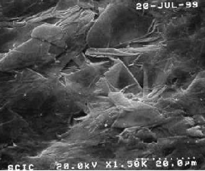
Figure 1: Typical rough graphite surface [62].

The $C_{60}$ molecule occupies the central place among fullerenes. This molecule resembles the commonly-used surface of a football. The carbon atoms are distributed on a spherical surface at the vertices of twenty regular hexagons and twelve regular pentagons. The radius of the $C_{60}$ molecule, deduced from X-ray structure analysis [56], is 0.357 nm. The common structural components found in graphite and the $C_{60}$ fullerene molecule determine the nature of the process of formation of fullerenes by the decomposition of graphite. Moderate heating of graphite breaks the bonds between the separate layers and an evaporated layer then splits into separate fragments. These fragments are combinations of hexagons one of which becams used to form a cluster.

The process of formation of fullerenes from graphite yields further various structures which are composed, like graphite, of six-member carbon rings. These structures are closed and empty inside. They include nanoparticles and nanotubes. The nanoparticles are closed structures similar to fullerenes, but of much larger size. In contrast to fullerenes, they may contain several layers. Such multilayer spherical structures are called onions. The study [55] of field emission properties of diamond-like carbon films indicate that the films have a faceted morphology with carbon cluster size in the range 150-400 nm. The fitting of I-F (current-electric field) data to the F-N equation gives $\beta_{{}_{FN}}\simeq$160, assuming $\varphi$ = 5 eV.

Carbon nanotubes (CNT) are elongated structures with surfaces formed by regular hexagons. Separate extended graphite fragments, which are then vent into a tube, form the base of CNT. These tubes are up to several microns long with diameters of a few nanometers. They are multilayer structures with rounded ends. One end is attached to a surface and the other is free.

As follows from direct measurements [57]-[63], CNT have quite a high field emission capability. This property centers around the extraordinarily small diameter of CNT, which provides a sizeable enhancement of the electric field strength near the CNT cap in relation to that averaged over the entire volume of the interelectrode gap. For instance, at a voltage near 650 V, an emitting area of about 1 mm² provides an emission current of order 0.5 mA. The measured emission characteristics correlate well with the F-N equation, with the condition that the value of the electric field strength is taken at the point of the electron emission. Since this point is situated close to the sharpened top of the CNT cap, the local magnitude of the electric field considerably exceeds its mean value. Thus, the above mentioned effect of field enhancement becomes involved, with the magnitude of $\beta_{{}_{FN}}$ estimated to be of the order of 1000, assuming the work function to be close to $\varphi$ = 5 eV.

High emission properties of CNT cannot be attributed only to their high aspect ratio. As demonstrated in model calculations and measurements [64, 65], single- and multiwalled CNT generate both IPS as discussed above and a new class of surface states, the tubular image states, owing to their quantized centrifugal motion. Measurements of binding energies and the temporal evolution of image state electrons were performed using femtosecond time-resolved photoemission. A cluster of IPS with n=1 is located near 0.75 eV below the vacuum level. These data are in agreement with results obtained in the course of studies of the emission properties of CNT [60, 66]. The values of the effective work function calculated from the Fowler-Nordheim plot are in the range 0.3 $-$ 1.8 eV and the highest value of $\beta_{{}_{FN}}$ extracted from the data is of the order of 1300.

3 The Electric Field of Relativistic Charges

3.1 Single Charged Particle

The electric field of a charged particle at rest is spherically symmetric. If the particle is moving with a uniform velocity ${\bf v}$ in an inertial frame ${\bf S}$, its electric field is deformed: along the direction of motion the electric field becomes weaker by a factor $\gamma^{2}$, while in the transverse direction the electric field is enhanced by a factor $\gamma$. Here, $\gamma$ denotes the particle Lorentz factor.

Let $(x,y,z)$ be the coordinates and ${\bf\vec{r}}$ the position vector of the point P in ${\bf S}$, the z-axis of the frame being taken along the direction of motion of the charged particle. Then the components of the electric field produced by a rapidly moving charge $q$ are [16], [17]

$$\vec{F}\,=\,\frac{\kappa\,q\,\gamma}{[x^{2}+y^{2}+\gamma^{2}(z-vt)^{2}\,]^{3/2}}\,(x,y,z-vt),$$ (19)

where the value of $\kappa$ depends on the system of units used, in our case $\kappa=1$ . We use the particle charge $q$ rather than the elementary charge $e$ to include particles with multiple charges such as ions for which $q=Ze$. At $t=0$ and $z=r\,cos\,\theta$, where $\theta$ is the angle which the vector ${\bf\vec{r}}$ makes with the z-axis, equation (19) can be rewritten in the form

$$\vec{F}\,=\,\kappa\frac{q\,\gamma}{r^{2}}\Big{[}\frac{1-\beta^{2}}{1-\beta^{2}\,sin^{2}\,\theta}\Big{]}^{3/2}\,\frac{\bf\vec{r}}{r},\hskip 14.22636pt\vec{B}\,\sim\vec{\beta}\times\vec{F}.$$ (20)

Thus, the magnitude of the electric field at $\theta\,=\,0^{\circ}$ or $\theta\,=\,180^{\circ}$, $F_{\parallel}$, is given by

$$F_{\parallel}\,=\,\kappa\frac{q}{\gamma^{2}\,r^{2}},$$ (21)

while in the transverse direction, the magnitude of the electric field is

$$F_{\perp}\,=\,\kappa\frac{q\,\gamma}{r^{2}}.$$ (22)

As seen from Eq.(22), the increase of the strength of the electric field in the transverse direction corresponds efficiently to an increase of the particle electric charge, $Q_{eff}=\gamma Ze$.

In accelerators, charged particles move in front of conducting surfaces and one has to account for the image charge induced by the particle. In this section we discuss only the case when a positively charged particle is moving parallel to a grounded conducting plane. The particle and the image charge form a dipole. The complete form of the electric field vector of the relativistic dipole is presented in Appendix .

Let the surface of the conductor coincide with the (y,z)-plane and (0,y,z) be a point on the plane. The electric field at this point is normal to the surface and is directed into it. The components of the field from a positive point charge, located at the distance $h$ above the plane, are (see Appendix)

$$\vec{F}\,=\,\frac{2\kappa q\gamma}{\big{[}h^{2}+y^{2}+\gamma^{2}(z-vt)^{2}\big{]}^{3/2}}(-h,0,0).$$ (23)

Thus, at $t$=0 the magnitude of the electric field at the point directly beneath the positive charge is

$$F_{\perp}\,=\,\frac{2\kappa q\gamma}{h^{2}}.$$ (24)

We find that accounting for the image charge doubles the electric field strength on the surface.

From equation (24) we conclude that only particles with ultra-high energies are able to produce significant field strengths at macroscopic distances. Let us substitute in (24) the numerical values of constants. That gives

$$F_{\perp}\,=\,2.88\cdot 10^{-7}\frac{Z\gamma}{h^{2}}\,,$$ (25)

where $h$ is the transverse distance in cm, $F$ is the electric field in V/cm. For instance, the field strength of 1 V/cm at a distance 1 cm from the particle is generated by a positron of energy 1.75 TeV or a proton of energy $3.25\cdot 10^{3}$ TeV. Thus, only particles of ultra-high energies (e.g. cosmic rays) are capable to generate a large field strength at macroscopic distances.

3.2 Bunch of Charged Particles

Let us consider a bunch of $N$ positively charged particles uniformly distributed within a circular cylinder of length $L$. Suppose that the bunch axis is along the coordinate z-axis and the bunch is moving along the z-axis with a relativistic velocity $\vec{v}=c\vec{\beta}$. The radial electric self-field of such a rapidly moving bunch is described by [18]

$$F_{\perp}(r,z)\,=\,\kappa\frac{qN\gamma}{rL}\Big{\{}\frac{z}{\sqrt{r^{2}+\gamma^{2}z^{2}}}\Big{(}1+\frac{3}{8}\frac{b^{2}}{r^{2}}C^{2}_{1}\Big{)}+\frac{L-z}{\sqrt{r^{2}+\gamma^{2}(l-z)^{2}}}\Big{(}1+\frac{3}{8}\frac{b^{2}}{r^{2}}C^{2}_{2}\Big{)}\Big{\}}$$ (26)

with

$$C_{1}\,=\,\Big{[}1+\frac{\gamma^{2}z^{2}}{r^{2}}\Big{]}^{-1},\ \ \ \ C_{2}\,=\,\Big{[}1+\frac{\gamma^{2}(L-z)^{2}}{r^{2}}\Big{]}^{-1}.$$ (27)

The field described by (26), has a different behavior at distances far apart from the bunch and in the near region, $r\leq L$. At very large distances, $r\gg\gamma z$ and $r\gg\gamma(L-z)$, equation (26) reduces to the Coulomb form (22). At the same time, in the near region and beyond the bunch tails, $\gamma z\approx\gamma(L-z)\gg r$ and equation (26) simplifies to

$$F_{\perp}\,=\,\kappa\frac{2qN}{L}\frac{1}{r},$$ (28)

which coincides with the external field of a continuous beam with the linear charge density $\lambda=qN/L$.

In an accelerator, a charged beam is influenced by its an environment (beam pipe, magnets, collimators, etc.), and a high-intensity bunch induces surface (image) charges or currents into this environment. This modifies the electric and magnetic fields around the bunch. For instance, if the bunch is moving in the midplane between infinitely wide conducting planes at $x=\pm h$ (this simple geometry models a collimator gap), then the transverse component of the bunch electric field is described by [18]

$$F_{\perp,tot}(x)\,=\,\kappa\frac{2qN}{Lh}\cdot\frac{\pi/2}{\sin(\frac{\pi}{2}\delta)}.$$ (29)

where $\delta=x/h$. Thus, on the surface, $\delta=1$, the field is enhanced by a factor $\pi/2$ due to the presence of the conducting planes. If the bunch is displaced in the horizontal plane by $\bar{x}$ from the midplane the resulting field behaves as [18]

$$F_{\perp,tot}(x,\bar{x})\,=\,\kappa\frac{2qN}{Lh}\cdot\Big{[}\frac{\pi}{2}\cdot\frac{\cos(\frac{\pi}{2}\bar{\delta})}{\sin(\frac{\pi}{2}\delta)-\sin(\frac{\pi}{2}\bar{\delta})}-\frac{\bar{\delta}}{\delta-\bar{\delta}}\Big{]}.$$ (30)

Here $\bar{\delta}=\bar{x}/h$. Equations (28)-(30) demonstrates that although in the relativistic limit the electric field does not depend on $\gamma$, the field strength may be very high if $N$ is large and the product $Lh$ is small.

4 Field Emission in HEP Colliders

In Section 2 the conditions were described under which FE starts to develop. Let us examine in this section the performance of the Large Hadron Collider (LHC) and the US Linear Collider (USLC) [67], in an attempt to display their ”bottlenecks”. In the following, we shall not consider well established locations such as RF superconductive cavities, where FE routinely occurs and leads to the rapid growth of power dissipation with field. Our consideration here is limited to locations where bunches are moving close to conducting surfaces and create electric fields strong enough to activate observable FE effects. For the analysis we need to know the beam parameters, distances to the closest surfaces, their shapes, and materials their constituent.

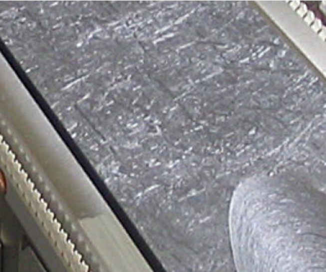
Figure 2: View from the close distance to the LHC collimator jaw surface [79].

4.1 The LHC Collimator System

Each of the two LHC rings will store 2808 bunches, each bunch populated with $N=1.15\cdot 10^{11}$ protons at energies of up to 7 TeV (nominal design parameters). To handle the high intensity LHC beams and the associated high loss rates of protons, a strongly acting collimator system was designed and constructed [77]-[83]. The LHC collimators must restrict the mechanical aperture in the machine and clean the primary halo so that quenches of magnets are avoided. To provide the required beam quality at the interaction points, primary and secondary collimators must be physically close to the high intensity beams. This impose strong limitations on the materials of the jaws and the length of the jaws. In the ”final” solution for the collimation system [83], [84], the collimators in IR3 and IR7 (and IR6) are made of graphite with parallel jaw surfaces and small gaps, $\sim$2 mm, at 7 TeV. Therefore, the first candidate for a bottleneck is the very narrow collimator gap.

Different scenarios for the beam parameters are foreseen in the LHC operation. These parameters are listed in Table 1 [85]. For the nominal scenario, in accordance with (29), the field strength at a distance of 1 mm from a bunch is equal 69 KV/cm. At this field level FEC is negligible if calculated with use of the classical FN equation (4). However, the surface of a jaw made of graphite may be polished only mechanically and the resulting surface roughness is high (see Fig 2). The surface roughness and many other surface effects as discussed in Section 2 are characterized by the field enhancement parameter $\beta_{{}_{FN}}$, whose actual value needs to be determined by direct measurements. Thereby, the calculations of FEC presented below are performed for a range of $\beta_{{}_{FN}}$ values. The FEC density, $J_{{}_{FN}}(\beta_{{}_{FN}}F,T)$, calculated for the graphite jaws with use of (29) and (12) at $T$=300 K, $h$=0.1 cm and $\varphi$=4.6 eV is shown in Fig. 1. For $\beta_{{}_{FN}}$ below 300 and the nominal scenario (LHC-n), the electron emission is negligible. FEC for $\beta_{{}_{FN}}$ in the range 300-500 begins to be notable and at higher $\beta_{{}_{FN}}$ may became a very serious problem. In the advanced scenarios (LHC-0/1), when bunches are twice as short and their population is higher by the factor 1.48 (the field level on the surface increases by the factor 2.94), the emission current at $\beta_{{}_{FN}}$=200 increases by 14 orders of magnitude ! At higher $\beta_{{}_{FN}}$, a very dense electron flow will cause electrical breakdown in vacuum, jaw surface heating and damage. The electron flow could also disturb the proton beam trajectory and give rise to loss of protons. The current density depicted in Fig. 1 can be translated into the number emitted electrons, $N_{e}$. A bunch with parameters from Table 1, expose the area $\delta\!A=2L\cdot\sigma^{*}$ during the time $\tau=L/c$ will extract from both jaw surfaces $N_{e}=2\delta\!A\tau J$ electrons. That gives $N_{e}=7.93\cdot 10^{7}J$ for LHC-n and $N_{e}=1.36\cdot 10^{7}J$ for LHC-0/1, respectively. Fig. 2 shows the evolution of $N_{e}$ with $\beta_{{}_{FN}}$. We note that at $\beta_{{}_{FN}}\approx$520 the number of extracted electrons $N_{e}$(LHC-n) is comparable with the number of protons per bunch.

Table 1

LHC Beam Scenarios [85, 86, 87]
bunch parameters	Nominal	Phase 0	Phase 1	”Super-bunch”
bunch population, N	1.15$\times 10^{11}$	1.7$\times 10^{11}$	1.7$\times 10^{11}$	5.6$\times 10^{14}$
bunch radius, $\sigma^{*}$	16.7 $\mu$m	11.3 $\mu$m	-	-
bunch length, $L$	7.55 cm	3.78 cm	3.78 cm	7500 cm
beam energy	7 TeV	7.45 TeV	7.45 TeV	7 TeV

Figure 3: Densities of the electron current emitted from a graphite collimator jaw at $T$=300 K,
$\varphi$=4.6 eV for the different beam scenarios.

Figure 4: The number of electrons extracted by a single bunch from jaw surfaces at $T$=300 K,
$\varphi$=4.6 eV and $h$=0.1 cm for the different beam scenarios.

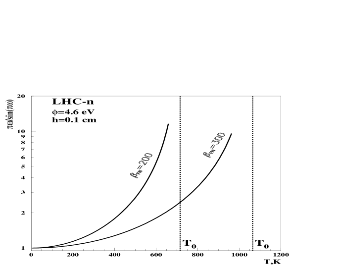
Figure 5: The temperature increment of the FE current (12) at different $\beta_{{}_{FN}}$ in the temperature
range as restricted by the conditions (14)-(15). $T_{0}$ denotes the temperature limit as determined
from (13).

Figure 6: Densities of the electron current ejected from the copper beam screen at $T$=20 K:
(LHC-n, LHC-0/1) due to presence of the surface image-potential states (IPS), $\varphi$(IPS)= 0.92 eV,
LHC-sb) the super-bunch scenario , $\varphi$(Cu)= 4.65 eV.

The FE current rises not only with $F_{eff}$, but the number of active emitters also increases with the field. A local increase of the emission current causes Joule heating of the emission tip which in turn leads to an increase of FEC. Fig. 3 illustrates the effect. It shows the temperature dependent factor in (12), whose rise is limited by the conditions (14) and (15). For a given field strength and higher temperatures it is necessary to apply equations of the thermo-field-emission theory [5, 6].

Joule heating by FEC is not the only mechanism responsible for an abrupt increase of FEC. Many studies point out that other mechanisms are also responsible for melting or damage of the emitter, such as the bombardment of the surface by ions. These ions are created by FEC as it passes through a cloud of gas evolving from the emission site [26, 27]. The plasma that develops can create an electric field on the order of 10⁷ V/cm at its interface with the conducting wall and may result in an explosion of the emitter [28]-[31],[20].

In Section 2 we noted that the image potential states on the surface of solids are characterized by low values of the work function, $\varphi<$ 1 eV. If we hypothesize that the field emission due to IPS contributes in an important way to FEC, then the inner beam screen, consisting of copper tubes lining the LHC vacuum chamber, is another candidate for a bottleneck. Indeed, the proton beam is moving at a distance of $\sim$2 cm away from the beam screen wall with cryopumping slots [91, 92], whose sharp edges could be very effective emission sites with high $\beta_{{}_{FN}}$. Fig. 4 shows the dependence of the FEC density on $\beta_{{}_{FN}}$ calculated with $\varphi$=0.92 eV, $h$=2cm and $T$=20 K, the temperature at which the beam screen will be maintained. As seen from the figure, for the LHC-n scenario IPS electrons will be seen only if $\beta_{{}_{FN}}>$500. However, in the LHC-0/1 scenario emission will be large already if $\beta_{{}_{FN}}\sim$150 or higher. At $\beta_{{}_{FN}}\approx$ 600 the top of the surface potential barrier is located below the energy level of IPS with n=1. These electrons escape the surface freely and this is reflected as a change in the slope of the curve. In Fig 6 also shown calculations for the super-bunch scenario (see Table 1) with the nominal work function for cooper, $\varphi$= 4.65 eV.

The results presented in Fig 6 are to some extent speculative. The calculations were performed assuming that the density of IPS electrons, pumped by the soft component of the synchrotron radiation from the bulk to the surface is of the same order as the density of electrons at the Fermi level. Nevertheless they give rise to a cause for concern that FE from the beam screen may amplify electron cloud formation.

4.2 The US Linear Collider

In the similar way we may evaluate the level of the field emission in other colliders, for example proposed US superconducting linear collider (USLC) [67] which can became a prototype of a future international linear collider (ILC). The USLC will bring into collision electrons and positrons at energy $\sqrt{s}$=500 GeV or, after an energy upgrade, 1000 GeV. The vacuum chamber in the positron ring will be coated throughout with a material with low secondary electron yield (e.g. conditioned titanium nitride, TiN) to prevent build-up of electron cloud. The beam pipe has a circular internal cross-section, with radius $h$=21 mm. The vacuum chambers are all constructed from an aluminum alloy. The bunch length is extraordinary short. The bunch compressors must reduce the $\sim$5 mm rms length of the bunches extracted from the damping rings to 300 $\mu$m bunch length required for the main linac and final focus systems. For optimum collider performance in the cold option, bunches with a charge of $N=2.0\cdot 10^{10}$ and a length of $L=300\mu$m will be injected for acceleration in the main linac.

For a beam well centered in the circular beam pipe, the image charge effect is vanished [68]. For this reason, instead of (29) we use in calculations equation (28). As a result, the electric field strength on an ideal smooth surface is characterized by the parameter $N/hL$. Direct calculations shows that

$$\Big{(}\frac{N}{hL}\Big{)}_{{}_{USLC}}>\frac{\pi}{2}\Big{(}\frac{N}{hL}\Big{)}_{{}_{LHC}},$$ (31)

denoting that with the same $\beta_{{}_{FN}}$ and $\varphi$ as for the LHC, the field emission from the USLC beam pipe surface will be stronger than in the LHC collimators. Fig. 7 shows the FE current density predicted for a variety of $\varphi$ values. The range of $\varphi$ employed in the calculations reflects uncertainties in the work function of TiN reported by different authors [69]-[76]. There is an observation [70], that changing the nitrogen concentration can modify the work function of TiN. Furthermore, a thickness dependency of the work function was observed for TiN/Al [71]. For a TiN layer with thickness less than 20 angstroms, the TiN/Al gate work function is the same as reported Al work-function (about 4.08 eV). For TiN layers of thickness greater than 100 angstroms, the TiN/Al gate work function is approximately the same as reported TiN work-function (4.5 V). For TiN layers with thickness from 20 angstroms to 100 angstroms, the work function can change as the TiN thickness is changed. The TiN crystal orientation is important because the metal work function is strongly dependent on this quantity. According to [72], (100) orientation TiN has $\varphi\simeq$4.6 eV and 4.4 eV in the (111) orientation. The work function of the TiN film was found to be sensitive to the film morphology, stipulated by a sputtering technology and may be as low as 3.72 eV [73].

In this way, the uncertainty in the value of $\varphi$ gives rise to an uncertainty in the current density of 3-5 orders of magnitude.

We finally point out that parameters of the positron and proton bunches and the beam pipe geometry at the HERA collider are such that even at $\beta_{{}_{FN}}=10^{3}$ the emission current density is well below $10^{-17}$ A/cm².

Figure 7: Densities of the electron current emitted from the USLC main linac beam pipe at $T$=20 K
and various values of the work function.

Figure 8: Energy distributions of the emitted electrons for the four values of the surface temperature. The curves are drawn according to (17).

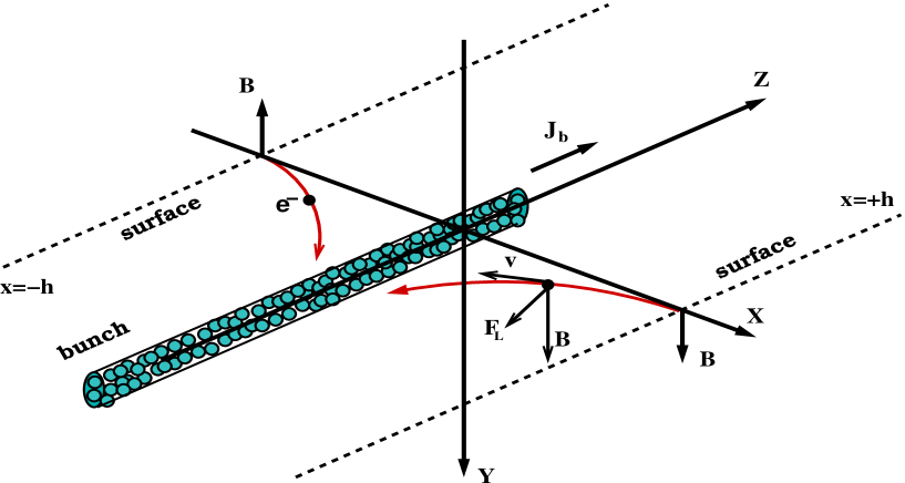
Figure 9: Illustration to Eq. (32). Electrons ejected from the surface with the velocity $\mathbf{v}=(\mathtt{v_{x}},0,0)$ are accelerated in the radial electric field and rotated by the magnetic field $\mathbf{B}$, created by a cylindrical proton bunch. The Lorentz force acting on the electron is denoted by $\mathtt{\mathbf{F}_{L}}$ and the beam current by $\mathbf{J_{b}}$.

5 Electron Dynamics in the Bunch Fields

In this section we discuss in a semiquantitative way the fate of electrons after their emission in the LHC collimator gap. Electrons leaves the surface with different energies. The energy spectra of electrons just ejected by the surface is presented in Fig 8. For a given imposed field, the width of the energy distribution grows with an increase of the surface temperature and more energetic electrons easier escapes the emitter.

Let us consider a single electron motion in the self-fields of a bunch. The analysis is based on the classical Lorentz equation [88, 89, 90]

$$\frac{d\vec{p}}{dt}\,=\,e\vec{F}+ec[\vec{\beta}^{(e)}\times\vec{B}].$$ (32)

To be specific, assume that the electron is emitted from the plane surface with the velocity vector, $\vec{\beta}^{(e)}=\vec{v}^{(e)}/c$, normal to the surface. The surface is placed parallel to the ($0,\,y,\,z$) plane at a distance $x=+h$. The bunch is moving along the line (0,0,z) in the positive $z$ direction, as shown in Fig. 9. In the simple geometry chosen, we consider, only as an illustration, the evolution of an electron trajectory in the ($x,\,0,\,z$) plane; in this way components of the self-field vectors can be set $\vec{F}=(F_{x},0,0)$ and $\vec{B}=(0,B_{y},0)$, where $F_{x}$ is of the form (29) and [18]

$$B_{y}\,=\,\frac{\kappa}{c}\frac{2qN}{Lh}\Big{[}\frac{B_{{}_{f}}}{\delta}+(1-B_{{}_{f}})\frac{\pi/2}{\sin(\frac{\pi}{2}\delta)}\Big{]}\cdot\beta^{(b)}_{\!z}.$$ (33)

Here $\beta^{(b)}_{z}$ is the $z$-component of the bunch velocity, $\delta=x/h$, $B_{{}_{f}}=\sqrt{2\pi}L/2\pi R$ is the Laslett bunching factor and $R$ the average LHC machine radius. In the LHC-n scenario, $B_{{}_{f}}=7.05\times 10^{-6}$ [93, 94] and terms proportional to $B_{{}_{f}}$ can be omitted in (33).

Surface irregularities of a very small size possess tips that cause a local field enhancement and increased emission. The field of such a tip decays with distance approximately as [10]

$$M(\delta)=1+\beta_{{}_{FN}}\Big{(}\frac{\rho}{\rho+h|1-\delta|}\Big{)}^{2},$$ (34)

where $\delta=x/h$ is a normalized distance from the emission tip, $\rho$ the tip radius. The self-fields $\vec{F}$ and $\vec{B}$ enter equation (32) multiplied by the factor (34).

For numerical calculations, it is convenient rewrite (32) by use the dimensionless time $\tau=t/\tau_{0}$ with $\tau_{0}=L/c$. For a full generality, we retain a relativistic treatment of equation (32) which in components becomes

$$\frac{d(\beta^{(e)}_{x}\gamma^{(e)})}{d\tau}\, = \,(1-\beta^{(e)}_{z}\beta^{(b)}_{z})\cdot\mathcal{F}(\delta),$$

$$\frac{d(\beta^{(e)}_{z}\gamma^{(e)})}{d\tau}\, = \,-\beta^{(e)}_{x}\beta^{(b)}_{z}\cdot\mathcal{F}(\delta),$$ (35)

where the function $\mathcal{F}(\delta)$ outside the bunch takes the form

$$\mathcal{F}(\delta)=\mathcal{A}\cdot\frac{M(\delta)}{\sin(\frac{\pi}{2}\delta)},\ \ \ \ \ \sigma^{*}<|x|\leq h,$$ (36)

and inside the bunch is [18]

$$\mathcal{F}(\delta)=\frac{2\mathcal{A}}{\pi}\Big{(}\frac{h^{2}}{{\sigma^{*}}^{2}}+\frac{\pi^{2}}{24}\Big{)}\delta,\ \ \ \ \ |x|\leq\sigma^{*}$$ (37)

with the dimensionless constant

$$\mathcal{A}=\frac{\kappa\pi}{mc}\frac{eqN}{Lh}\tau_{0}.$$

A direct estimation gives that $\mathcal{A}=O(1)$ for the LHC-n parameters. Fig 9 schematically shows electron trajectories and forces acting on the electron as a consequence of equation (32).

Let us analyze the system (35). For a relativistic bunch one may put $\beta^{(b)}_{z}=+1$ and therefore below we omit superscripts in the electron velocity components. A partial solution of (35) can be found for nonrelativistic electrons, $\gamma\simeq 1$, by taking a ration of the two equations. That gives

$$\beta_{x}\frac{d\beta_{x}}{d\tau}=(\beta_{z}-1)\frac{d\beta_{z}}{d\tau}.$$

After integration of the last equation and some algebra one finds a solution in the form

$$\beta_{z}=1-\sqrt{1+\beta^{2}_{x}-\beta^{2}_{0}}\,,$$

where the integration constant $\beta_{0}$ is fixed by initial conditions $\beta_{z}=$0, $\beta_{x}=\beta_{0}$ at $t$=0. This equation connects the $p_{z}$ and $p_{x}$ components of the electron momentum in the following way

$$p_{z}=-\frac{{p^{2}}_{\!\!\!{}_{x}}-{p^{2}}_{\!\!\!{}_{0}}}{2mc}.$$ (38)

Equation (38) implies that during the electron acceleration $p_{z}$ remains negative and much smaller than $p_{x}$. Thus, the electron displacement in the $z$ direction is expected to be small too.

The magnetic field of the bunch gives rise to the $p_{z}$ component and the electron turn in the ($x$,0,$z$) plane. For an accelerated charge the radiation emitted at any instant is approximately the same as that emitted by a particle moving instantaneously along the arc of a circular path whose radius of curvature is $R_{i}$. The frequency spectrum of radiation emitted by a charge in instantaneously circular motion is characterized by the critical frequency

$$\omega_{c}=\frac{3}{2}\frac{c}{R_{i}}\gamma^{3},$$ (39)

beyond which there is negligible radiation at any angle [88, 90]. The corresponding energy of the photon is $E_{{}_{\gamma}}=\hbar\omega_{c}$.

For a nonrelativistic charge whose motion is described by the system (35) with $\gamma^{(e)}=1$, the instantaneous radius $R_{i}$ can be found in the following way. Let the point ($x_{0}$, $z_{0}$) be the center of the circle of radius $R_{i}$

$$(x-x_{0})^{2}+(z-z_{0})^{2}={R^{2}}_{\!\!i}$$ (40)

whose infinitesimal arc with the point ($x$, $z$) on it coincide at the moment $\tau$ with the electron trajectory. To find $R_{i}$ we differentiate (40) twice by $\tau$ and find relations between $x-x_{0}$, $z-z_{0}$ and $\beta_{x}$, $\beta_{z}$, $\dot{\beta_{x}}$ and $\dot{\beta_{z}}$. Using (35) for $\dot{\beta_{x}}$ and $\dot{\beta_{z}}$, we obtain

$$R_{i}(\tau)=\frac{c\tau_{0}\beta^{3}}{|\mathcal{F}(\delta)|(\beta^{2}_{x}-\beta^{2}_{z}+\beta_{z})}.$$ (41)

Now we are in a position to present numerical results. The input parameters for a numerical solution of the system (35) are listed in Table 2. These are the distance, $h$, from the bunch center to the collimator plane, the tip radius $\rho$ in equation (34), the field enhancement factor at the surface, $\beta_{{}_{FN}}$, the electron velocity $\beta$, or its kinetic energy $E_{{}_{kin}}$. Parameters of the proton beam are correspond to the LHC-n scenario, see Table 1.

Table 2

Input paramerets for the system (35)
$h$, mm	$\rho$, m	$\beta_{{}_{FN}}$	$E_{{}_{kin}}$, eV	$\beta_{x}$	$\beta_{z}$
1	1.0$\times 10^{-8}$	300	4.6	-4.2$\times 10^{-3}$	0.0

Table 3 presents parameters of the electron trajectory, whose numerical values were calculated at the emission point ($\delta$=1), at the bunch center ($\delta$=0) and at the opposite collimator plate ($\delta=-$1). The trajectory is split into three parts. At the first stage, the electron is accelerating by the field (36) and moves toward the bunch (Fig 9). The local field enhancement (34) causes an extremely high acceleration rate and a rapid increase of the electron momentum. At the start time the instant curvature of the trajectory $R_{i}$ is very small and the energy loss $E_{{}_{\gamma}}$ through radiation can run up to 5% of the initial electron energy. At later times with an increase in the distance from the surface, the energy loss by radiation is very low, $E_{{}_{\gamma}}\sim 10^{-6}-10^{-4}$ eV.

At the second stage, the electron is crossing the bunch. The internal field of the bunch is described by (37). At the bunch center the electron momentum reaches a maximum value of 151 KeV/c at $\tau=$0.129 after emission. An average distance between protons in the LHC-n bunch is of the order of 100 nm and the electron either passes through the bunch or will

Table 3

Selected paramerets of the electron trajectory
$\delta$	$\tau$	$\beta$	$E_{{}_{kin}}$, eV	p, KeV/c	$R_{i}$, m	$\omega_{c}$, Hz	$E_{{}_{\gamma}}$, eV	$\sqrt{s_{ep}}$, GeV
1	0	4.2$\times 10^{-3}$	4.6	2.17	1.1$\times 10^{-6}$	4.3$\times 10^{14}$	0.283	-
0	0.129	0.293	2.3$\times 10^{4}$	151.0	7.7$\times 10^{-2}$	6.7$\times 10^{9}$	4.4$\times 10^{-6}$	2.94
-1	0.254	3.3$\times 10^{-2}$	271.1	16.6	4.8$\times 10^{-3}$	9.5$\times 10^{10}$	6.2$\times 10^{-5}$	-

be scattered by a proton. In the later case, the electron and the proton undergo an elastic or inelastic collision at the center of mass energy of 2.94 GeV. In the rest frame of the proton, the electron carries the momentum of 4.13 GeV/c. Such an amount of energy is enough for hadron production in an inelastic $ep$ collision.

At the last stage, the electron is decelerated by the bunch field. If the electron passes the bunch without scattering, then at the moment when $\tau=$0.254 it impacts the opposite plate of the collimator at $\delta=$-1 with a kinetic energy of 271 eV. For a fully symmetric configuration and neglecting the electron energy loss in the course of acceleration and deceleration, the electron has to arrive at the opposite plate with the same kinetic energy as at the start point. The energy difference arise due to an additional acceleration of the electron in the enhanced field at the tip apex and the assumption that at the end point the surface is flat.

Above, we considered the emission of a single electron, when at $\tau$=0 the emission point and the bunch head had the same z-coordinate. However, the field emission occurs throughout the entire region $L$, covered by the field of the bunch. Each electron reaches the bunch center after time $\Delta\tau\approx$ 0.129. If now account a bunch movement, then electrons emitted at $1-2\Delta\tau<\tau<1$, will experience only initial acceleration or deceleration in the wake field of the bunch. Thus, the electron energy spectrum will be very broad, from 4.6 eV to 23 KeV. As a result of emission from both collimator plates, the proton bunch occurs in the electron streams being intersected. For high $\beta_{{}_{FN}}$ it is necessary take into account the space charge of electron clouds, whose electric field reduces the the strength of the bunch field and leads to a decrease of the electron emission. Nevertheless, the leading part of the bunch of length $\Delta\tau$ will always remains out of the electron cloud and triggers the field emission.

The interaction between the electron and the surface results in the ejection of secondary electrons from the material. The secondary electrons consist of true secondaries and those elastically reflected. The number of secondary electrons is given by the secondary emission coefficient (SEC) that depends on the surface characteristics and on the impact energy of the primary. In turn, the secondaries are accelerated and, on impact, produce further generation of electrons. The electron-cloud build-up is sensitive to the intensity, spacing, and length of the proton bunches. The electron flow increases exponentially if the number of emitted electrons exceeds the number of impacting electrons, and if their trajectories satisfy some specific conditions. For most materials the SEC exceeds unity for impact energies in a range from a few tens of eV to a few thousand of eV. This type of electron multiplication, so-called multipacting, and build-up a cloud of electrons has been studied recently very intensively [91]-[104]. In the LHC arcs, as believed, the dominant source of electrons will be photo-electrons from synchrotron radiation and beam-induced multipacting to be the leading source of sustained electron-production.

The region near the scrapers and collimators is susceptible to a high beam-loss, and is potentially another location of high electron concentration. Protons incident on the collimator surfaces produce secondary electrons. Depending on the energy of the beam and the incident angle, the secondary electron-to-proton yield can greatly exceed unity when the incident beam is nearly parallel to the surface.

In conclusion let us note that any heterogeneous structures such as a grooved metal surface [105, 106] introduced with intention to combat with the multiplication of electrons and located near an intensive positively charged beam, may in real conditions actually provoke field emission.

6 Praemonitus Praemunitus

The analysis performed in the previous sections makes it possible to draw the conclusion that in the addition to the known electron sources, electron field emission intensified by multipacting can make a dominant contribution to the build-up of an electron cloud in the LHC collimator system and may become a serious problem. The analysis of the ILC prototype reveals that a noticeable field emission will accompany positron bunches on their entire path during acceleration.

From the examples considered we learn that the level of field emission is controlled by two essential parameters. The first of these, $\beta_{{}_{FN}}$, is wholly determined by the state of the emitting surface and by the processes proceeding on it. Therefore, control of $\beta_{{}_{FN}}$ is possible only within certain limits. The effect of surface aging will increase $\beta_{{}_{FN}}$ with time. The actual value of $\beta_{{}_{FN}}$ for the graphite jaw can be obtained only by direct measurement.

For $\beta_{{}_{FN}}$ below 300 and the nominal LHC-n scenario, the electron emission is negligible. If the $\beta_{{}_{FN}}$ value is in the range of 300-500, FEC begins to be notable. At higher $\beta_{{}_{FN}}$, FEC may became a very serious problem. In the advanced scenarios (LHC-0/1), when bunches are twice as short and their population is higher by a factor 1.48, the emission current at $\beta_{{}_{FN}}$=200 increases by 14 orders of magnitude as compared with LHC-n. At higher $\beta_{{}_{FN}}$, a very dense electron flow will cause electrical breakdown in vacuum, jaw surface heating and damage. The electron flow could also disturb the proton beam trajectory and give rise to a loss of protons.

The value of the second parameter, N/hL, is assigned by the beam parameters and the distance to the conducting surface. It is possible and necessary to choose the components of $\beta_{{}_{FN}}$N/hL in the way to minimize the electron field emission.

Acknowledgments. The author is grateful to P. Bussey, P.F. Ermolov, E. Lohrmann, E.B. Oborneva, V.I. Shvedunov and A.N. Skrinsky for useful discussions and comments. A special thanks goes to O. Brüning whose talk [85] stimulated the interest of the author to problems discussed in the paper.

Appendix: Electric Field of a Relativistic Dipole

Take two point charges, +q and -q, separated by a distance $2h$. The charges are at rest in frame ${\bf\bar{S}}$ and the $\bar{x}$-axis passes through the charges. We denote the coordinates of a point in the frame ${\bf\bar{S}}$ by $(\bar{x},\bar{y},\bar{z})$. Then the potential from the two charges (a dipole) is given by

$$\varphi(\bar{x},\bar{y},\bar{z})\,=\,\kappa\Big{\{}\frac{q}{\sqrt{(\bar{x}-h)^{2}+\bar{y}^{2}+\bar{z}^{2}}}-\frac{q}{\sqrt{(\bar{x}+h)^{2}+\bar{y}^{2}+\bar{z}^{2}}}\Big{\}}.$$ (A-1)

We obtain the electric field of a dipole at rest by the usual rule:

$$\vec{F}\,=\,-\,\vec{\nabla}\varphi$$ (A-2)

or in components

$$\bar{F}_{x}=\kappa q\Big{[}\frac{\bar{x}-h}{\bar{D}^{3}_{-}}\,-\,\frac{\bar{x}+h}{\bar{D}^{3}_{+}}\Big{]},\ \ \ \bar{F}_{y}=\kappa q\Big{[}\frac{1}{\bar{D}^{3}_{-}}\,-\,\frac{1}{\bar{D}^{3}_{+}}\Big{]}\,\bar{y},\ \ \ \bar{F}_{z}=\kappa q\Big{[}\frac{1}{\bar{D}^{3}_{-}}\,-\,\frac{1}{\bar{D}^{3}_{+}}\Big{]}\,\bar{z},$$ (A-3)

where

$$\bar{D}_{\pm}\,=\,\sqrt{(\bar{x}\pm h)^{2}+\bar{y}^{2}+\bar{z}^{2}}.$$ (A-4)

Now, suppose that the dipole is moving along the z-axis of the frame ${\bf S}$ with velocity $v$. Then the space coordinates in ${\bf S}$ and ${\bf\bar{S}}$ are related by the Lorentz equations

$$\bar{x}\,=\,x,\ \ \ \bar{y}\,=\,y,\ \ \ \bar{z}\,=\,\gamma(z-vt),$$ (A-5)

The transformation laws for the components of the electric field can be written as

$$F_{x}\,=\,\gamma\bar{F}_{x},\ \ \ F_{y}\,=\,\gamma\bar{F}_{y},\ \ \ F_{z}\,=\,\bar{F}_{z}.$$ (A-6)

Substituting expressions of $\bar{F}$ from (A-3) into (A-6) and account (A-5), we arrive at

$$F_{x} = \kappa q\gamma\Big{[}\frac{x-h}{D^{3}_{-}}\,-\,\frac{x+h}{D^{3}_{+}}\Big{]}$$ (A-7)

$$F_{y} = \kappa q\gamma\Big{[}\frac{1}{D^{3}_{-}}\,-\,\frac{1}{D^{3}_{+}}\Big{]}\,y$$ (A-8)

$$F_{z} = \kappa q\gamma\Big{[}\frac{1}{D^{3}_{-}}\,-\,\frac{1}{D^{3}_{+}}\Big{]}\,(z-vt),$$ (A-9)

where

$$D_{\pm}\,=\,\sqrt{(x\pm h)^{2}+y^{2}+\gamma^{2}(z-vt)^{2}}.$$ (A-10)

On the plane $x=0$

$$F_{x}\,=\,-\,\frac{2\kappa q\gamma h}{\big{[}h^{2}+y^{2}+\gamma^{2}(z-vt)^{2}\,\big{]}^{3/2}},\ \ \ F_{y}\,=\,F_{z}\,=\,0.$$ (A-11)

References

- [1] R.P.Little and W.T. Whitney, Electron emission preceding electrical breakdown in vacuum, J. Appl. Phys. 34 (1963) 2430.
- [2] R. W. Wood, A new form of cathode discharge and the production of X-rays, together with some notes on diffraction, Phys. Rev. (Series I) 5, (1897) 1-10.
-
[3]
R.H. Fowler and L.W. Nordheim, Proc. Roy. Soc.(London) 119 (1928) 173.
L.W. Nordheim, Proc. Roy. Soc.(London) 121 (1928) 626.
L. Nordheim, Die Theorie der Electronenemission der Metalle, ”Physikalische Zeitschrift”, Bd. 30, N 7, (1929) 117. - [4] A. Sommerfeld, H. Bethe, Elektronentheorie der Metalle, Springer-Verlag, 1967.
- [5] E.L. Murphy and R.H. Good, Jr, Phys. Rev. 102 (1956) 1464.
- [6] S.G. Christov, Surf. Sci., 70 (1978) 32.
- [7] R.H. Good jr. and E. W. Müller, Field Emission, in: Encyclopedia of Physics, Vol. XXI, S. Flügge (Ed.), 1956.
- [8] M.I. Elinson and G.F. Vasiliev, Autoelectron emission (in Russian), M, 1958.
- [9] V.N. Shrednik, in ”Cold cathodes” (in Russian), Ed. M.I. Elinson, M, 1974.
- [10] R. Gomer, Field Emission and Field Ionization, AIP, NY, 1993.
- [11] A. Modinos, Field, Thermionic, and Secondary Electron Emission Spectroscopy, Plenum Press, NY, 1983.
- [12] P.W. Hawkes and E. Kasper, Theory of electron emission, in: Princeples of Electron Optics, Vol. 2, Academic Press, 1996.
- [13] S. Eidelman et al., Review of Particle Physics, Phys. Lett. B592 (2004) 1.
- [14] R.E. Burgess, H. Kroemer and J.M. Houston, Phys. Rev. 90 (1953) 515.
- [15] B.B. Levchenko, On parametrizations of the Nordheim function, E arXiv:cond-mat/0512513, 2005.
- [16] M. Saleem and M. Rafique, Special Relativity: Applications to Particle Physics and the Classical Theory of Fields, Ellis Horwood, 1993.
- [17] R.P. Feynman, R.B. Leighton and M. Sands, The Feynman lectures on physics, Definitive edition, v.2, Addison Wesley, 2005.
- [18] B.B. Levchenko, Real and Image Fields of a Relativistric Bunch, DESY report 06-094, 2006; E arXiv:physics/0604013, 2006.
- [19] T.J. Lewis, High field electron emission from irregular cathode surfaces, J. Appl. Phys. 26 (1955) 1405.
- [20] I.N. Slivkov, Electrical Insulation and a Vacuum Discharge (in Russian), Atomizdat, M., 1972.
- [21] H.A. Schwettman J.P. Turneare and R.F. Waites, Evidence for surface-state-enhanced field emission in rf superconducting cavities, L. Appl. Phys. 45 (1974) 914.
- [22] R.J. Noer, Electron field emission from broad-area electrodes, Appl. Phys. A 28 (1982) 1.
- [23] M. Jimenez et al., Electron field emission from large-area cathodes: evidence for the projection model, J. Phys. D: Appl. Phys. 27 (1994) 1038.
- [24] N.S. Xu, Y. Tzeng and R.V. Lathman, J. Phys. D 27 (1994) 1988.
- [25] Vacuum Arcs, Theory and Applications,Ed. J.M. Laffetry, Wiley, NY., 1980.
- [26] J. Knobloch and H. Padamsee, Microscopic investigation of field emitters located by thermometry in 1.5 GHz superconducting niobium cavities. Part. Accel. 53(1996) 53.
-
[27]
J. Knobloch, Advanced Thermometry Studies of Superconducting RF Cavities, Ph.D thesis,
1997, http://www.lns.cornell.edu/public/CESR/SRF/dissertations
/knobloch/knobloch.html . - [28] E.A. Litvinov, G.A. Mesyats, D.I. Proskourovsky, Field emission and explosive electron emission processes in vacuum discharges, Soviet Physics Uspekhi, 26(2) (1983) 138.
- [29] G.N. Fursey, Field emission and vacuum breakdown, IEEE Transaction on Electrical Insulation EI-20(4), (1985) 659.
- [30] E.A. Litvinov, Theory of explosive electron emission, IEEE Transaction on Electrical Insulation EI-20(4), (1985) 683.
- [31] F.R. Schwirzke, Vacuum breakdown on metal surfaces, IEEE Transaction on Plasma Science 19(5), (1991) 690.
- [32] C.B. Duke and M.E. Alferieff, Field emission through atoms adsorbed on a metal surface, J. Chem. Phys. 46 (1967) 923.
- [33] J. Halbritter, Enhanced electron emission and its reduction by electron and ion impact. IEEE Transc. Electr. Insul. EI-!*(3) (1983) 253.
- [34] Q.S. Shu et al., Influence of condensed gases on field emission and the performance of superconducting rf cavities, IEEE Transactions on Magnetics. Proc. 14-th Applied Superconductivity Conf. MAG-25 (1989) 1868.
- [35] S.H. Jo et al., Field emission of carbon nanotubes grown on carbon cloth, Appl. Phys. Lett. 85 (2004) 810.
- [36] I.E. Tamm, Z. Phys. 76 (1932) 849.
- [37] W. Shockley, On the Surface States Associated with a Periodic Potential, Phys. Rev. 56, (1939) 317.
- [38] P.M. Echenique and J.B. Pendry, The existance and detection of Rydberg states at surfaces, J. Phys. C., 11 (1978) 2065.
- [39] Ansgar Liebsch, Electronic Excitations at Metal Surfaces, Premium Press, NY,
- [40] M. Prutton, Introduction to Surface Physics, Clarendon Press, Oxford, 1994.
- [41] J. R. Smith, J. G. Gay, and F. J. Arlinghaus, Self-consistent local-orbital method for calculating surface electronic structure: Application to Cu (100), Phys. Rev. B 21 (1980) 2201.
- [42] P. Heimann, J. Hermanson, H. Miosga, and H. Neddermeyer, d-like surface-state bands on Cu(100) and Cu(111) observed in angle-resolved photoemission spectroscopy,Phys. Rev. B 20 (1979) 3059.
- [43] H.J. Kreuzer, Surface Physics and Chemistry in High Electric Fields, in: Chemistry and Physics of Solid Surfaces VIII, Springer Ser. Surf. Sci., Vol. 22, Eds. R. Vanselov, R. Howe, (Springer, Berlin, 1990) p. 133.
- [44] J.H. Block, Field Desorption and Photon-Induced Feild Desorption, in:Chemistry and Physics of Solid Surfaces IV, Springer Ser. Chem. Phys., Vol. 20, Eds. R. Vanselov, R. Howe, (Springer, Berlin, 1982) p. 407.
- [45] H.D. Hangstrum, Surface Electronic Interactions of Slow Ions and Metastable Atoms, in: Chemistry and Physics of Solid Surfaces VII, Springer Ser. Surf. Sci., Vol. 10, Eds. R. Vanselov, R. Howe, (Springer, Berlin, 19??) p. 341.
- [46] D. Straub and F.J. Himpsel, Identification of image-potential surface states on metals, Phys. Rev. Lett. 52 (1984) 1922
- [47] U. Höfer, Self-trapping of electrons at surfaces , Science, 279 i. 5348 (1998) 190.
- [48] U. Höfer et al., Time-resolved coherent photoelectron spectroscopy of quantized electron states on metal surfaces, Science, 277, i. 5331 (1997) 1480.
- [49] P.M. Echenique et al., Decay of electronic excitations at metal surfaces, Surf. Sci. Rep. 52 (2004) 219.
- [50] J. Lehmann et al. Properties and dynamics of the image potential states on graphite investigated by multiphoton photoemission spectroscopy. Phys. Rev. B 60 (1999) 17037.
- [51] A.V. Eletskii and B.M. Smirnov, Fullerenes and carbon structures, Phys-Usp., 38 (1995) 935.
- [52] A.V. Eletskii, Carbon nanotubes, Phys-Usp., 40 (1997) 899.
- [53] A.V. Eletskii, Carbon nanotubes and their emission properties, Phys-Usp., 45 (2002) 369.
- [54] C.E. Hunt and Yu Wang, Application of vitreous and graphitic large-area carbon surfaces as field-emission cathodes, Appl. Surf. Sci. 251 (2005) 159.
- [55] A.H. Jayatissa, F. Sato and N. Saito, Enhanced field emission current from diamod-like carbon films deposited by laser ablation of C fullerene, J. Phys. D: Appl. Phys. 32 (1999) 1443.
- [56] W. Krätschmer, K. Fostiropolos, D. Huffman, Chem. Phys. Lett. 170 (1990) 167.
- [57] W. De Heer et al., in Fullerenes and Fullerene Nanostructures, Eds H. Kuzmany et al., Singapure: World Scietific, 1996, p. 215.
- [58] A.G. Rinzler et al. Science 269 (1995) 1550.
- [59] L.A. Chernozatonskiî et al., Chem Phys. Lett. 233 (1995) 63.
- [60] V.V. Zhirnov, E.I. Givargizov, and P.S. Plekhanov, Field emission from silicon spikes with diamond coatings, J. Vac. Sci. Technol. 13 (1995) 418.
- [61] V.I. Merkulov et al., Field-emission studies of smooth and nanostructured carbon films, Appl. Phys. Lett. 75 (1999) 1228
- [62] Z.F. Ren et al., Progress on production of carbon nanotubes, in Proc. 32-nd Int. SAMPE Techn. Conf. Nov. 2000, p.200.
- [63] Y. Cho, G. Kim, S. Lee and J. Ihm, Field emission of carbon nanotubes and the electronic structure of fullerenes encapsulated in carbon nanotubes, In ”Technical Proc. of the 2002 Int. Conf. on Computational Nanoscience and Nanotechnology”, Nanotech 2002, p. 291.
- [64] M.Zamkov et al., Time-Resolved Photoimaging of Image Potential States in Carbon Nanotubes, Phys. Rev. Lett. 93 (2004) 156803.
- [65] M.Zamkov et al., Image-potential states of single and multiwalled carbon nanotubes, Phys. Rev B70 (2004) 115419.
- [66] D. Carnahan, M. Reed, Z. Ren and K. Kempa, Field emission arrays of carbon nanotubes, See on the page http:// www.nano-lab.com/publications.html
-
[67]
U.S. Linear Collider Technology Options Study, SLAC, 2004,
http://www.slac.stanford.edu/xorg/accelops/ - [68] L.J. Laslett, On intensity limitations imposed by transverse space-charge effects. Rept. BNL-7534, Brookhaven National Laboratory, 1963. In ”Selected Works of J.Jackson Laslett”, Lawrence Berkeley Laboratory, University of California, PUB-616, Vol. III, 1987.
- [69] V.S. Fomenko and G.V. Samsonov, Handbook of Thermionic Properties (Plenum Press, New York, 1966) .
- [70] H. Wakabayashi, Y. Saito, K. Takeuchi, T. Mogami, and T. Kunio, in Technical Digest of IEEE International Electron Device Meeting (1999) 253.
- [71] Zheng et al Work function tuning for MOSFET gate electrodes, United States Patent, 6.373.111, 2002.
- [72] A. Yagishita et al. Improvement of threshold voltage deviation in damascene metal gate transistos, IEEE Trans. Electron Devices, 20 n 12 (1999) 632.
- [73] B.R. Rogers, Underlayer work function effect on nucleation and film morphology of chemical vapor deposited aluminum, Thin Solid Films 408 (2002) 87.
- [74] J. Westlinder, G. Sjöblom, J. Olsson, Variable work function in MOS capacitors utilizing nitrogen-controlled TiNx gate electrodes, Microelectronic Engineering, 75 (2004) 389. http://portal.acm.org/citation.cfm?id=1061284.1061291
- [75] D. Park et al, ”SiON/Ta2O5/TiN Gate-Stack Transistor with 1.8nm Equivalent SiO2 Thickness,” International Electron Devices Meeting Technical Digest, pp. 381-384, December 1998.
- [76] A. L. Hanson et al, Electron emission from ion bombarded stainless-steel surfaces coated and noncoated with TiN and its relevance to the design of high intensity storage rings, J.Vac.Sci. Technol. A 19 (2001) 2116
-
[77]
LHC Design Report, Vol.1, Ch. 18 Beam Cleaning and Collimation System, p. 467.
http://ab-div.web.cern.ch/ab-div/Publications/LHC-DesignReport.html -
[78]
LHC Collimation Working Group,
http://lhc-collimation.web.cern.ch/lhc-collimation -
[79]
LHC Collimation Project, Pictures/Carbon-carbon jaw.
http://lhc-collimation-project.web.cern.ch/lhc-collimation-project - [80] R.W. Aßmann et al., Designing and Building a Collimation System for the High-Intensity LHC Beam, in: Proc. 2003 Part. Acc. Conf., Ed. J. Chew, 2003, p. 45.
- [81] R.W. Aßmann, Collimators and cleaning: Could this Limit the LHC Performance?, in: Proceedings ”LHC Performance Workshop- Chamonix XII”, (2003) 163.
- [82] O. Aberle et. all, LHC Collimation: Design and Results from Prototyping and Beam Tests, in: Proc. 2005 Part. Acc. Conf., Knoxville, Ed. C. Horak, 2005, p. 1078.
-
[83]
R.W. Aßmann, The LHC Collimation System, AB Seminar, 10.03.2005,
http://lhc-collimation-project.web.cern.ch/lhc-collimation-project
/files/ab-seminar-mar05-a.pdf -
[84]
Basic Design Parameters and Location for Collimators in the LHC,
http://lhc-collimation-project.web.cern.ch/lhc-collimation-project . - [85] O. Brüning, The LHC Collider: Basics and machine physics challenges, DESY seminar, 24.05.2005.
- [86] O. Brüning et al, LHC Luminosity and energy upgrade : A Feasibility Study, CERN-LHC-Project Report-626, 2002.
- [87] M. Benedikt et al, Report of the High Intensity Protons Working Group, CERN-AB-2004-022 OP/RF, 2004.
- [88] A.A. Sokolov and I.M. Ternov, Radiation from relativistic electron, AIP Transl. Ser., NY, 1986
- [89] L.D. Landau and E.M. Lifshitz, The classical theory of fields, Butterworth-Heinemann, 2002.
- [90] J.D. Jackson, Classical electrodynamics, John WileySons, Inc., 1999.
- [91] O. Gröbner, Overview of the LHC vacuum system, Vacuum, 60 (2000) 25.
- [92] J. Gollies, Electron Clouds with Copper Linings, CERN Courier, 39, 6 (1999)
- [93] F. Ruggiero, Single-beam collective effects in the LHC, CERN SL/95-09, 1995.
-
[94]
LHC Design Report, Vol.1, Ch. 5 Collective Effects, p. 97.
http://ab-div.web.cern.ch/ab-div/Publications/LHC-DesignReport.html - [95] R. Cimino, I.R. Collins, M.A. Furman, M. Pivi, F. Ruggiero, G. Rumolo and F. Zimmermann, Can Low-Energy Electrons Affect High Energy Physics Accelerators?, Phys. Rev. Lett. 93 (2004) 014801.
- [96] O. Gröbner, Technological Problems Related to the Cold Vacuum System of the LHC, Vacuum, 47 (1996) 591.
- [97] O. Gröbner, Beam induced multipacting, (1998) 3589.
- [98] G. Arduini et al., Present Understanding of Electron Cloud Effects in the Large Hadron Collider, CERN, LHC Proj. Rep. 645, 2003.
- [99] O. Brüning et al., Electron Cloud and Beam Scrubbing in the LHC, in: Proc. 1999 Part. Acc. Conf., New York, Eds. A. Luccio, W. MacKay, 1999, p.2629.
-
[100]
Electron Cloud in the LHC,
http://ab-abp-rlc.web.cern.ch/ab%2Dabp%2Drlc%2Decloud/ - [101] M. Blaskiewicz, Electron Cloud Effect in Present and Future High Intensity Hadron Machines, in: Proc. 2003 Part. Acc. Conf., Ed. J. Chew, 2003, p.302.
-
[102]
J. Wei and R. Macek, Electron Cloud Effect in High-Intensity Proton accelerators,
in: Proc. ECLOUD’02 mini-workshop, CERN-2002-001, 2002
http://wwwslap.cern.ch/collective/ecloud02/ - [103] J. Wu et al., Electron-Cloud Effects in Transport Lines of a Normal Conducting Linear Collider, in: Proc. 2005 Part. Acc. Conf., Knoxville, Ed. C. Horak, 2005, p. 2527.
- [104] F. Zimmermann, Overview of LHC Electron-Cloud Effects & Present Understanding, CARE CERN-GSI bilateral meeting, March 30-31, 2006
- [105] G. Stupakov, M. Pivi, Suppression of the Effective Secondary Emission Yield for a Grooved Metal Surface, LCC-0145, SLAC-TH-04-045, 2004.
- [106] M.T.F. Pivi et al., Suppressing Electron Cloud in Future Linear Colliders, in: Proc. 2005 Part. Acc. Conf., Knoxville, Ed. C. Horak, 2005, p. 24.