Fluid dynamics at arbitrary Knudsen on a base of Alexeev-Boltzmann equation: sound in a rarefied gas

Abstract

The system of hydrodynamic-type equations is derived from Alexeev’s generalized Boltzmann kinetic equation by two-side distribution function for a stratified gas in gravity field. It is applied to a problem of ultrasound propagation and attenuation. The linearized version of the obtained system is studied and compared with the Navier-Stokes one at arbitrary Knudsen numbers. The problem of a generation by a moving plane in a rarefied gas is explored and used as a test while compared with experiment. It is good agreement between predicted propagation speed, attenuation factor and experimental results for a wide range of Knudsen numbers

Introduction

Fluid mechanics equations in its’ most popular form (Euler, Navier-Stokes, Fourier-Kirchhoff,Burnett, etc) appear in methods based on Boltzmann kinetic equation by means of expansion in Knudsen number(Kn). The first important version of such theory was made by Hilbert. It implies analiticity in Kn of both distribution function as well as momenta functions. Further development of the theory by Chapman-Enskog and Grad [1] weaken analiticity condition of the momenta on Kn. It allowed to deride NS, Burnett equations for the Chapman-Enskog method and 13 momenta Grad equations widely used in fluid dynamics description. Failures in deep Knudsen regime penetration recovered by direct attempts with many-moment theories lead to more deep understanding of the problem [2, 3, 4]. The Knudsen independent expansion of the basic (Boltzmann) equation was used, namely one of Gross-Jackson, starting from the celebrating BGK model. The unification of Chapman-Enskog and Gross-Jackson approaches[5] exploits an idea of nonsingular perturbation method in its Frechet expansion form [6].

One of important verification of fluid dynamics system relates to the problem of sound propagation. Its simplest version considers the plane harmonic wave with the correspondent dispersion relation. Such case obtained by linearization of the basic system reproduces the known experiments of [7] rather well. It incorporated in a direct scheme of kinetic approach [8]. The fluid mechanics systems, based on BGK [9] model of collision integral, obtained recently in [5] and [10], give good results for velocity of sound in Kn $0.1\div 10$ but fail in attenuation description [11].

Developing the method based on Gross-Jackson collision integral for a non-isotropic fluid for a problem, which specifies [12] a direction in it we use an idea of von Karman to divide the phase speed with respect of particle velocity direction along/against the direction axis [13]. Such situation takes place if a gas is stratified in gravity field, that yields appearance of interne gravity waves branch with the obvious necessity to account wide range of Kn [14].

Struchtrup [15] regularizes 13-moment Grad equations doing the same thing as a test. His linearization results in a dispersion relation, which acoustic branch gives an attenuation coefficient that also does not fit experiments.

Our article is devoted to this problem; we tried to improve the results on a way of next Gross-Jackson model [16], the tendency was good but the changes were not enough. Considering an alternative possibility to compensate the discrepancy in relaxation timeestimation, we adress to the Alexeev generalization of Boltzmann equation [17].

Alexeev-Boltzmann equation looks like:

$$\frac{Df}{Dt}-\frac{D}{Dt}\left(\tau\frac{Df}{Dt}\right)=J^{B}\ ,$$ (1)

where $\frac{D}{Dt}=\frac{\partial}{\partial t}+\vec{V}\frac{\partial}{\partial\vec{r}}+\frac{\vec{F}}{m}\frac{\partial}{\partial\vec{V}}$ is the substantional(particle) derivative, $\vec{V}$ and $\vec{r}$ are the velocity and radius vector of the particle, respectively, $\tau$ is the mean time between collisions, $J^{B}$ is the collision Boltzmann integral.

We apply our method for the generalized Boltzmann equation of Alexeev and such ”joint” theory gives a better agreement with the experimental data [7] for attenuation at arbitrary Knudsen number.

Generalized fluid dynamics equations

Consider the kinetic equation with the model integral of collisions in BGK form [9]:

$$J^{B}=\nu\left(f_{\it l}-f\right),\$$ (2)

here

$$f_{\it l}=\displaystyle\frac{n}{\pi^{3/2}v_{\scriptscriptstyle T}^{3}}\exp\left(-\frac{(\vec{V}-\vec{U})^{2}}{v_{\scriptscriptstyle T}^{2}}\right)$$

- local- equilibrium distribution function. $v_{\scriptscriptstyle T}=\sqrt{2kT/m}$ denotes the average thermal velocity of particles of gas, $\nu=\nu_{0}\exp(-z/H)$ – is the effective frequency of collisions between particles of the gas at height $z$, $H=kT/mg$ – is a parameter of the gas stratification. It is supposed, that density of the gas n, its average speed $\vec{U}=(U_{x},U_{y},U_{z})$ and temperature $T$ are functions of time and coordinates.

Following the idea of the method of piecewise continuous distribution functions let’s search for the solution $f$ of the equations(1) as a combination of two locally equilibrium distribution functions, each of which gives the contribution in its own area of velocities space:

$$f(t,\vec{r},\vec{V})=\left\{\begin{array}[]{rcl}f^{+}&=&\displaystyle n^{+}\left(\frac{m}{2\pi kT^{+}}\right)^{3/2}\exp\left(-\frac{m(\vec{V}-\vec{U}^{+})^{2}}{2kT^{+}}\right)\ ,\qquad v_{z}\geq 0\vspace{1mm}\\ f^{-}&=&\displaystyle n^{-}\left(\frac{m}{2\pi kT^{-}}\right)^{3/2}\exp\left(-\frac{m(\vec{V}-\vec{U}^{-})^{2}}{2kT^{-}}\right)\ ,\qquad v_{z}<0\\ \end{array}\right.$$ (3)

here $n^{\pm},U^{\pm},T^{\pm}$ depending on $t,z$ are functional parameters.

The double number of parameters of the distribution function results in its deviations from a local-equilibrium one. In the range of small Knudsen numbers $Kn<<1$ we should have $n^{+}=n^{-}$,$T^{+}=T^{-}$, $U^{+}=U^{-}$ and distribution function start from a local equilibrium and at the small difference between the functional ’up’ and ’down’ parameters produces the Navier-Stokes equations. The theory is also valid at big Kn(free molecular regime)[18].

We restrict ourselves by the case of one-dimensional disturbances $\vec{U}=(0,0,U)$, using a set of linearly independent momenta functions:

$$\begin{array}[]{rclrrcl}\varphi_{1}&=&m\ ,&\varphi_{4}&=&mV_{z}^{2}\ ,\vspace{2mm}\\ \varphi_{2}&=&mV_{z}\ ,&\varphi_{5}&=&\displaystyle mV_{z}V^{2}\ ,\vspace{2mm}\\ \varphi_{3}&=&\displaystyle\frac{1}{2}mV^{2}\ ,&\varphi_{6}&=&\displaystyle mV_{z}^{3}\ .\\ \end{array}$$ (4)

Here the first three functions are collisional invariants. Let’s define a scalar product in velocity space:

$$<\varphi_{n},f>\equiv<\varphi_{n}>\equiv\int d\vec{v}\>\varphi_{n}f\ .$$ (5)

$$\begin{array}[]{lll}<m>=\rho\ ,&<mV_{z}>=\rho U\ ,&<\frac{1}{2}m\xi^{2}>=\frac{3}{2}\frac{\rho}{m}kT\ ,\\ <m\xi_{z}^{2}>=P_{zz}\ ,&<\frac{1}{2}m\xi_{z}\xi^{2}>=q_{z},&<\frac{1}{2}m\xi_{z}^{3}>=\displaystyle\bar{q}_{z}.\\ \end{array}$$ (6)

where $\vec{\xi}=\vec{V}-\vec{U}$ is the peculiar velocity. Here $\rho=nm$ is mass density, $P_{zz}$ is the diagonal component of the pressure tensor, $q_{z}$ is a vertical component of a heat flux vector, $\bar{q}_{z}$ is a parameter having dimension of the heat flux.

If we now multiply the kinetic equation with the model integral of collisions in BGK form by $\varphi_{i}$ and integrate over velocity space, the fluid dynamic equations appear:

$$\begin{array}[]{l}\displaystyle\frac{\partial}{\partial t}\rho+\frac{\partial}{\partial z}(\rho U)-\tau\frac{\partial^{2}}{\partial^{2}t}\rho-2\tau\frac{\partial^{2}}{\partial t\partial z}(\rho U)-\tau\frac{\partial^{2}}{\partial^{2}z}(P_{zz}+\rho U^{2})=0\ ,\vspace{2mm}\\ \displaystyle\frac{\partial}{\partial t}\rho U+\frac{\partial}{\partial z}(P_{zz}+\rho U^{2})-\tau\frac{\partial^{2}}{\partial^{2}t}(\rho U)-2\tau\frac{\partial^{2}}{\partial t\partial z}(P_{zz}+\rho U^{2})-\tau\frac{\partial^{2}}{\partial^{2}z}(2\bar{q}_{z}+3UP_{zz}+\rho U^{3})=0\ ,\vspace{2mm}\\ \displaystyle\left(\frac{\partial}{\partial t}-\tau\frac{\partial^{2}}{\partial^{2}t}\right)(\frac{\rho U^{2}}{2}+\frac{3}{2}\frac{\rho}{m}kT)+\left(\frac{\partial}{\partial z}-2\tau\frac{\partial^{2}}{\partial t\partial z}\right)(\frac{\rho U^{3}}{2}+U\frac{3}{2}\frac{\rho}{m}kT+UP_{zz}+q_{z})-\vspace{1mm}\\ \displaystyle-\tau\frac{\partial^{2}}{\partial^{2}z}\left(\frac{\rho U^{4}}{2}+2U(q_{z}+\bar{q}_{z})+U^{2}(\frac{3}{2}\frac{\rho}{m}kT+\frac{5}{2}P_{zz})+<\frac{m}{2}\xi_{z}^{2}\xi^{2}>\right)=0\ ,\vspace{2mm}\\ \displaystyle\left(\frac{\partial}{\partial t}-\tau\frac{\partial^{2}}{\partial^{2}t}\right)(\rho U^{2}+P_{zz})+\left(\frac{\partial}{\partial z}-2\tau\frac{\partial^{2}}{\partial t\partial z}\right)(\rho U^{3}+3P_{zz}U+2\bar{q}_{z})-\vspace{1mm}\\ \displaystyle-\tau\frac{\partial^{2}}{\partial^{2}z}\left(\rho U^{4}+8U\bar{q}_{z}+6P_{zz}U^{2}+<m\xi_{z}^{4}>\right)=\nu(\frac{\rho}{m}kT-P_{zz})\ ,\vspace{2mm}\\ \displaystyle\left(\frac{\partial}{\partial t}-\tau\frac{\partial^{2}}{\partial^{2}t}\right)(\rho U^{3}+2P_{zz}U+3\frac{\rho}{m}kTU+2q_{z})+\left(\frac{\partial}{\partial z}-2\tau\frac{\partial^{2}}{\partial t\partial z}\right)(\rho U^{4})+\vspace{1mm}\\ \displaystyle+\left(\frac{\partial}{\partial z}-2\tau\frac{\partial^{2}}{\partial t\partial z}\right)(4U(q_{z}+\bar{q}_{z})+U^{2}(3\frac{\rho}{m}kT+5P_{zz})+<m\xi_{z}^{2}\xi^{2}>)-\vspace{1mm}\\ \displaystyle-\tau\frac{\partial^{2}}{\partial^{2}z}\left(U^{2}(6q_{z}+14\bar{q}_{z})+2<m\xi_{z}^{4}>U+3<m\xi_{z}^{2}\xi^{2}>U+<m\xi_{z}^{3}\xi^{2}>\right)-\vspace{1mm}\\ \displaystyle-\tau\frac{\partial^{2}}{\partial^{2}z}(\rho U^{5}+U^{3}(3\frac{\rho}{m}kT+9P_{zz}))=-2\nu q_{z}-2\nu U(P_{zz}-\frac{\rho}{m}kT)\ \ ,\vspace{2mm}\\ \displaystyle\left(\frac{\partial}{\partial t}-\tau\frac{\partial^{2}}{\partial^{2}t}\right)(\rho U^{3}+3P_{zz}U+2\bar{q}_{z})+\vspace{1mm}\\ \displaystyle+\left(\frac{\partial}{\partial z}-2\tau\frac{\partial^{2}}{\partial t\partial z}\right)(\rho U^{4}+8U\bar{q}_{z}+6P_{zz}U^{2}+<m\xi_{z}^{4}>)-\vspace{1mm}\\ \displaystyle-\tau\frac{\partial^{2}}{\partial^{2}z}\left(\rho U^{5}+10U^{3}P_{zz}+20U^{2}\bar{q}_{z}+5<m\xi_{z}^{4}>U+<m\xi_{z}^{5}>\right)=\vspace{1mm}\\ \displaystyle=-2\nu\bar{q}_{z}-3\nu U(P_{zz}-\frac{\rho}{m}kT),\end{array}$$ (7)

where

$$\begin{array}[]{ll}\displaystyle\quad J_{1}=\frac{m}{2}<\xi_{z}^{2}\xi^{2}>\ ,&J_{2}=\frac{m}{2}<\xi_{z}^{4}>\ ,\\ \displaystyle J_{3}=\frac{m}{2}<\xi_{z}^{5}>,&J_{4}=\frac{m}{2}<\xi_{z}^{3}\xi^{2}>\ .\\ \end{array}$$ (8)

The system (7) of the equations according to the derivation scheme is valid at all Kn. To close the description it is enough to plug the two-side distribution function into (6), that yields for $n^{\pm},U^{\pm},T^{\pm}$ as function of $\rho,U,T,P_{zz},q_{z},\bar{q}_{z}$. We base here on an expansion in small Mach numbers $M=max|\displaystyle\frac{U}{v_{T}}|\$, up to the first order. The values of integrals (8) as functions of thermodynamic parameters of the system (7) are:

$$\begin{array}[]{l}\displaystyle\quad J_{1}=-\frac{5}{2}\rho(\frac{kT_{0}}{m})^{2}+\frac{11}{4}{\frac{kT_{0}P_{zz}}{m}}+\frac{9}{4}(\frac{k}{m})^{2}\rho T_{0}T\ ,\\ \displaystyle J_{2}=-\frac{3}{2}\rho(\frac{kT_{0}}{m})^{2}+\frac{9}{4}{\frac{kT_{0}P_{zz}}{m}}+\frac{3}{4}(\frac{k}{m})^{2}\rho T_{0}T\ ,\\ \displaystyle J_{3}=6\frac{kT_{0}}{m}\bar{q}_{z}+\frac{kT_{0}}{m}q_{z}+4\rho_{0}U\frac{k^{2}T_{0}^{2}}{m^{2}}-4\rho U\frac{k^{2}T_{0}^{2}}{m^{2}}\ ,\\ \displaystyle J_{4}=6\frac{kT_{0}}{m}\bar{q}_{z}+3\frac{kT_{0}}{m}q_{z}+6\rho_{0}U\frac{k^{2}T_{0}^{2}}{m^{2}}-6\rho U\frac{k^{2}T_{0}^{2}}{m^{2}}.\end{array}$$ (9)

Substitute $J_{I}$ into (7) gives modification of fluid dynamics equations at arbitrary Knudsen numbers.

Let us report the results of investigation of quasi-plane waves parameters as a function of Kn. For this purpose we proceed in a standart way:linearizing the system (7) that impose the dispersion relation as a link between frequency and complex wave number.

In the model of hard spheres in the continual limit $\tau$ can be connected with the dynamical viscosity $\eta$ [2]

$$\tau p=0.786\eta.$$

$\tau$ and $\nu$ are linked :

$$\tau=0.786\nu.$$

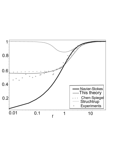
Figure 1: The inverse non-dimensional phase velocity as a function of the inverse Knudsen number. The results of this paper are compared to Navier-Stokes, Chen-Spiegel [10], regularization of Grad’s method [15] and the experimental data [7]

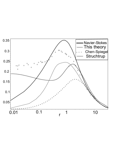
Figure 2: The attenuation factor of the linear disturbance as a function of the inverse Knudsen number.

In figures 1, 2 a comparison of our results of numerical calculation of dimensionless sound speed and attenuation factor depending on $r\sim\frac{1}{Kn}$ is carried out in a parallel way with the results by other authors. The Navier-Stokes prediction is qualitatively wrong at big Knudsen number. Our results for phase speed give the good consistency with the experiments at all Knudsen numbers. However, our results for the attenuation of ultrasound are good (as we can see in experiment) for the number r up to order unity and in the free molecular regime. Taking into account disadvantages of model integral of collisions it is planed to consider kinetic equation with full integral of collisions. It will permit to describe processes in transition regime.

References

• [1] H. Grad Communications on Pure and Applied Mathematics 2, N 4, 331-407 (1949).
• [2] S. Chapmann, T.G. Cowling, The Mathematical Theory of Non-Uniform Gases, third ed., Cambridge University Press, Cambridge, UK, 1970.
• [3] G.A. Bird Molecular Gas Dynamics and the Direct Simulation of Gas Flows, Clarendon Press, Oxford, England, 1994.
• [4] A.V. Bobylev, Sov. Phys. Dokl. 262, N 1, 71-75 1982.
• [5] S.B. Leble , D.A. Vereshchagin Advances in Nonlinear Acoustic (ed.H.Hobaek).Singapore. World Scientific. 1993. pp. 219-224.
• [6] S.B. Leble Nonlinear Waves in Waveguides with Stratification. Berlin: Springer-Verlag, 1990,164p.
• [7] E. Meyer , G. Sessler , Z.Physik 149. 15-39 ( 1957).
• [8] S.K. Loyalka, T.S. Cheng, Phys. Fluids.,22. N 5. 830-836 (1979).
• [9] E.P. Gross , E.A. Jackson , Phys. Fluids 2, N 4, 432-441 (1959)
• [10] E.A. Spiegel and J.-L. Thiffeault , Physics of Fluids, 15 (11), 3558-3567.(2003)
• [11] D.A. Vereshchagin, S.B. Leble, M.A. Solovchuk, Physics Letters A, 348 , 326-334.(2006)
• [12] L. Lees, J.Soc.Industr. and Appl.Math., 13,N 1, 278-311.(1965)
• [13] D.A. Vereshchagin, S.B. Leble. Nonlinear Acoustics in Perspective, ed. R.Wei. 142-146.(1996)
• [14] D.A. Vereshchagin, S.B. Leble, Piecewise continuous distribution function method: Fluid equations and wave disturbances at stratified gas , physics/0503233,(2005)
• [15] H. Struchtrup, M. Torrilhon, Phys.Fluids 15, N 9, 2668-2680 (2003)
• [16] S.B. Leble, M.A. Solovchuk. One-dimensional ultrasound propagation at stratified gas: Gross-Jackson model, physics/0607161 (2006)
• [17] B.V. Alexeev, Generalized Boltzmann Physical Kinetics, Elsevier, 2004
• [18] F. Sharipov , W. Jr.Marques , and G. M. Kremer , J. Acoust. Soc. Am. 112 (2), 395-401(2002)