Abstract

We consider the nonspherically decaying radiation field that is generated by a polarization current with a superluminally rotating distribution pattern in vacuum, a field that decays with the distance $R_{\rm P}$ from its source as $R_{\rm P}^{-1/2}$, instead of $R_{\rm P}^{-1}$. It is shown (i) that the nonspherical decay of this emission remains in force at all distances from its source independently of the frequency of the radiation, (ii) that the part of the source that makes the main contribution toward the value of the nonspherically decaying field has a filamentary structure whose radial and azimuthal widths become narrower (as $R_{\rm P}^{-2}$ and $R_{\rm P}^{-3}$, respectively), the farther the observer is from the source, (iii) that the loci on which the waves emanating from this filament interfere constructively delineate a radiation ‘subbeam’ that is nondiffracting in the polar direction, (iv) that the cross-sectional area of each nondiffracting subbeam increases as $R_{\rm P}$, instead of $R_{\rm P}^{2}$, so that the requirements of conservation of energy are met by the nonspherically decaying radiation automatically, and (v) that the overall radiation beam within which the field decays nonspherically consists, in general, of the incoherent superposition of such coherent nondiffracting subbeams. These findings are related to the recent construction and use of superluminal sources in the laboratory and numerical models of the emission from them. We also briefly discuss the relevance of these results to the giant pulses received from pulsars.

OCIS codes: 230.6080, 030.1670, 040.3060, 250.5530, 260.2110, 350.1270

1 Introduction

1.A Preamble

Maxwell’s generalization of Ampère’s law[1] establishes that electromagnetic radiation can be equally well generated by a time-dependent electric polarization current, with a density $\partial{\bf P}/\partial t$, as by a current of accelerated free charges with the density ${\bf j}$:

$$\nabla\times{\bf H}=\frac{4\pi}{c}{\bf j}+\frac{1}{c}\frac{\partial{\bf D}}{\partial t}=\frac{4\pi}{c}({\bf j}+\frac{\partial{\bf P}}{\partial t})+\frac{1}{c}\frac{\partial{\bf E}}{\partial t};$$ (1)

here, ${\bf E}$ and ${\bf H}$ are the electric and magnetic fields, ${\bf D}$ is the displacement and $c$ is the speed of light in vacuo. A remarkable aspect of the emission from such polarization currents is that the motion of the radiation source is not limited by $c$. Although the speed of charged particles cannot exceed $c$, nothing prevents the distribution pattern of a polarization current, created by the coordinated motion of subluminal particles, from moving faster than light.[2, 3, 4] Indeed, radiation from such superluminal polarization currents has been observed in the laboratory.[5, 6, 7, 8]

Since electric polarization arises from separation of charges, a polarization current is by its nature volume-distributed. In fact, no superluminal source can be point-like; for, if a point source were to move faster than its own waves, it would generate caustics on which the field strength would diverge.[2, 9]

There is growing experimental and theoretical interest in radiation by polarization currents whose distribution patterns move at a superluminal speed with acceleration.[8] One of the simplest implementations of such sources employs distribution patterns that have the time dependence of a traveling wave with circular superluminal motion; here, the acceleration is centripetal. We are investigating the use of polarization currents with such superluminally rotating distribution patterns in applications relating to communications and radar.[10, 6] Furthermore, one of the proposed models of the radio emission from pulsars postulates the presence of sources of this type in the magnetospheres of rapidly rotating neutron stars.[11, 12] The clarification of a diverse set of current questions, therefore, hinges on an understanding of the radiation from superluminal polarization currents undergoing circular motion [13, 14, 15].

Our purposes in the present paper are (i) to examine the geometry of those regions within such extended sources that make the dominant contribution toward the radiation field observed at a given point and time, and (ii) to identify the salient features Uof the angular distribution of this radiation. A detailed knowledge of the extent and geometry of the contributing part of the source is required not only for the efficient design of practical superluminal sources of this type (e.g. for the design of the dielectric in which the polarization current is generated),[6] but also for understanding the narrow widths of the giant pulses that are received from pulsars.[16] Likewise, a knowledge of the evolution of the angular distribution of the radiation with distance both facilitates the experimental detection of the tightly-beamed large-amplitude component of the emission from such sources and establishes a connection between two observed features (the nanostructure and the high brightness temperature) of the pulsar emission. [17, 18, 19, 20]

In Ref. 13, the field of a superluminally rotating extended source was evaluated by superposing the fields of its constituent volume elements, i.e. by convolving its density with the familiar Liénard-Wiechert field of a rotating point source. This Liénard-Wiechert field is described by an expression essentially identical to that which is encountered in the analysis of synchrotron radiation, except that its value at any given observation time receives contributions from more than one retarded time. The multivalued nature of the retarded time is an important feature of all superluminal emission; we shall begin, therefore, by describing the relationship between observation (reception) time and retarded (emission) time for the particular case of a rotating source with the aid of Fig. 1.

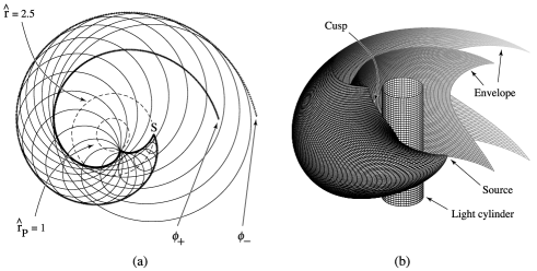
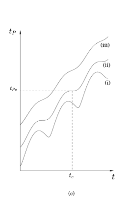
Fig. 1: (a) Cross-section of the Čerenkov-like envelope (bold curves) of the spherical Huygen’s wave fronts (fine circles) emitted by a small element ${\rm S}$ within an extended, rotating superluminal source of angular velocity $\omega$. S is on a circle of radius $r=2.5c/\omega$, or, in our dimensionless units, $\hat{r}\equiv r\omega/c=2.5$; i.e. its instantaneous linear velocity is $r\omega=2.5c$. The cross-section is in the plane of ${\rm S}$’s rotation; dashed circles designate the light cylinder $r_{\rm P}=c/\omega$ ($\hat{r}_{\rm P}=1$) and the orbit of ${\rm S}$. (b) Three-dimensional view of the light cylinder, the envelope of wave fronts emanating from ${\rm S}$, and the cusp along which the two sheets $\phi_{\pm}$ of this envelope meet tangentially. (c) The relationship between reception time $t_{\rm P}$ and source (retarded) time $t$ [ Eq. (4)] plotted for $\hat{r}=2.5$ and three different observation points. The maxima and minima of curve (i) occur on the sheets $\phi_{\pm}$ of the envelope, respectively. Curve (ii) corresponds to an observation point that is located on the cusp. Note that the waves emitted during an interval of retarded time centered at $t_{c}$ are received over a much shorter interval of observation time at $t_{P_{c}}$. Curve (iii) is for an observation point that is never crossed by the rotating sheets of the envelope. (After Ref. 13.)

1.B Multivalued retarded times, the cusp and temporal focusing

Parts (a) and (b) of Fig. 1 show the wave fronts that emanate from a small, circularly moving superluminal source ${\rm S}$. As we have already pointed out, no superluminal source can be truly pointlike. Here we are considering a volume element of an extended source whose linear dimensions are much smaller than the other length scales of the problem.

The emission of waves by any moving point source whose speed exceeds the wave speed is described by a Liénard-Wiechert field that has extended singularities. These singularities occur on the envelope of wave fronts where the Huygens wavelets emitted at differing retarded times interfere constructively and so form caustics. A well-understood example is the emission of acoustic waves by a point source that moves along a straight line with a constant supersonic speed. In this case, simple caustic forms along a cone issuing from the source, the so-called Mach cone, and most of the emitted energy is confined to the vicinity of this propagating ‘shock’ front. Another, similar example is the formation of the Čerenkov cone in the electromagnetic field of a uniformly moving point charge whose speed exceeds the speed of light inside a dielectric medium.

When the supersonic or superluminal motion of such sources is in addition accelerated, the simple conical caustic that occurs in the Mach or Čerenkov radiation is replaced by a two-sheeted envelope with a cusp.[21, 22, 9] The effect of acceleration is to give rise to a one-dimensional locus of observation points at which more than two simultaneously received wave fronts meet tangentially. The spherical wave fronts that are centered at the retarded positions of the source neighboring a point from which such coalescing wave fronts emanate cannot but be mutually tangential (in pairs) to two distinct surfaces, surfaces that constitute the separate sheets of a cusped envelope.

More specifically, the Čerenkov-like envelope that is generated by a uniformly rotating superluminal source consists of a tube-like surface whose two sheets meet, and are tangent to one another, along a spiraling cusp curve; this envelope is depicted in Fig. 1 and mathematically described in Eqs. (9)–(13) below. At any given observation time, three wave fronts pass through an observation point inside the envelope, while only one wave front passes through a point outside this surface. The envelope and its cusp are the loci of observation points at which, respectively, two or three of the simultaneously received wave fronts are tangential to one another. To specify the retarded times $t$ at which various wave fronts are emitted, let us adopt a cylindrical coordinate system based on the axis of rotation and denote the trajectory of the volume element ${\rm S}$, shown in Fig. 1, by

$$r={\rm const}.,\quad\varphi(t)=\hat{\varphi}+\omega t,\quad z={\rm const}.,$$ (2)

where $\hat{\varphi}$ denotes the initial value of $\varphi$, and $\omega$ is the angular velocity of ${\rm S}$. Let a stationary observer be positioned at a point ${\rm P}$, with cylindrical polar coordinates $(r_{\rm P},\varphi_{\rm P},z_{\rm P})$. The retarded-time separation $R(t)$ between the source volume element and the observer (i.e. their instantaneous separation at the time $t$ of emission) will therefore be

$$R(t)=[(z_{\rm P}-z)^{2}+r_{\rm P}^{2}+r^{2}-2rr_{\rm P}\cos(\varphi_{\rm P}-\hat{\varphi}-\omega t)]^{\frac{1}{2}}.$$ (3)

The relationship between the retarded time $t$ and the observation time $t_{\rm P}$, i.e.

$$t_{\rm P}=t+\frac{R(t)}{c},$$ (4)

is plotted in Fig. 1(c) for the source speed $r\omega=2.5c$ and for three classes of stationary observation points: those, located sufficiently close to the plane of rotation, that are periodically crossed by the two sheets of the rigidly rotating envelope [curve (i)], or by just the cusp curve of the envelope [curve (ii)], and those at higher latitudes that are never crossed by the envelope [curve (iii)].

The ordinates of the neighboring extrema of curve (i) in Fig. 1(c) designate those observation times, during each rotation period, at which the two sheets of the envelope go past the stationary observer [see Eqs. (6)–(9) below]. Thus, the field inside the envelope receives contributions from three distinct values of the retarded time [curve (i)], while the field outside the envelope is influenced by only a single instant of emission time [curves (i) and (iii)]. The constructive interference of the emitted waves on the envelope (where two of the contributing retarded times coalesce) and on its cusp (where all three of the contributing retarded times coalesce [curve (ii)]) gives rise to the divergence of the Liénard-Wiechert field on these loci. There is a higher-order focusing of the waves, and so a higher-order mathematical singularity, on the cusp than on the envelope itself. While the singularity that occurs on the envelope is integrable, that which occurs on the cusp is not. In that it occurs in the temporal as well as the spatial domain, this focusing is distinct from that produced by a conventional horn, mirror or lens. The enhanced amplitude on the cusp is due to the contributions from emission over an extended period of source time reaching the observer over a significantly shorter period of observation time.

The Liénard-Wiechert field derived in Ref. 13 was used as the Green’s function for calculating the emission from a superluminal polarization current, comprising both poloidal and toroidal components, whose distribution pattern rotates (with an angular frequency $\omega$) and oscillates (with a frequency $\Omega$) at the same time.[13] It was found that the convolution of the density of this current with the Green’s function described above results in a field that decays nonspherically: a field whose strength diminishes with the distance $R_{\rm P}$ from the source as $R_{\rm P}^{-1/2}$, rather than $R_{\rm P}^{-1}$, within the bundle of cusps that emanate from the constituent volume elements of the source and extend into the far zone. This result, which has now been demonstrated experimentally,[6, 7] was derived in Ref. 13 by setting the observation point within the bundle of generated cusps and evaluating the convolution integrals over various dimensions of the source.[13] The steps in this procedure are listed below.

1. The integration with respect to the azimuthal extent of the source was performed by means of Hadamard’s method.[23, 24] It was shown that the Hadamard finite part of the divergent integral that describes the field of a superluminally rotating ring with a sinusoidal density distribution consists of two parts: one part is exclusively contributed by the two elements on the ring that approach the observer along the radiation direction with the speed of light at the retarded time (i.e. the elements for which ${\rm d}R/{\rm d}t=-c$), and the other part is contributed by the entire extent of the ring.

2. The integration with respect to the radial dimension of the source was subsequently performed by the method of stationary phase.[25]

It was found that, when the radiation frequency is much higher than the rotation frequency $\omega$, the main contribution toward the field of a superluminally rotating annular ring comes from the vicinity of the point on the ring that approaches the observer not only with the wave speed, but also with zero acceleration (i.e. the point at which ${\rm d}R/{\rm d}t=-c$ and ${\rm d}^{2}R/{\rm d}t^{2}=0$ simultaneously).

These contributing source elements are the ones for which the time-domain phase $t_{\rm P}=t+R(t)/c$ is doubly stationary. Differentiating Eq. (4) with respect to $t$, we can see that

$$\frac{{\rm d}R}{{\rm d}t}=-c\qquad{\rm and}\qquad\frac{{\rm d}^{2}R}{{\rm d}t^{2}}=0$$ (5)

are equivalent to

$$\frac{{\rm d}t_{\rm P}}{{\rm d}t}=0\qquad{\rm and}\qquad\frac{{\rm d}^{2}t_{\rm P}}{{\rm d}t^{2}}=0.$$ (6)

These conditions jointly define the point of inflection in curve (ii) of Fig. 1(c), corresponding to the cusp passing through the point of observation ${\rm P}$.

The collection of volume elements satisfying Eq. (5) within an extended source has a filamentary locus that is approximately parallel to the axis of rotation for an observation point located in the far zone (Fig. 2). The nonspherically decaying field that is generated by a volume-distributed source arises almost exclusively from the elements in the vicinity of this narrow filament, a filament whose position within the source depends on the location of the observer.

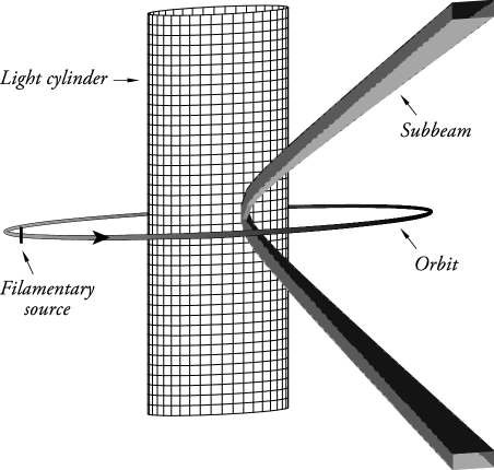
Fig. 2: Schematic illustration of the light cylinder $r=c/\omega$, the filamentary part of the source that approaches the observeration point with the speed of light and zero acceleration at the retarded time, the orbit of this filamentary source, and the subbeam formed by the bundle of cusps that emanate from the constituent volume elements of this filament. The subbeam is diffractionless in the direction of $\theta_{\rm P}$. The figure represents a snapshot corresponding to a fixed value of the observation time $t_{\rm P}$. The polar width $\delta\theta_{\rm P}$ of this subbeam decreases with the distance $\hat{R}_{\rm P}$ in such a way that the thickness $\hat{R}_{\rm P}\delta\theta_{\rm P}$ of the subbeam in the polar direction remains constant: It equals the projection, $\delta\hat{z}\sin\theta_{\rm P}$, of the $\hat{z}$ extent, $\delta\hat{z}$, of the contributing filamentary source onto a direction normal to the line of sight. The azimuthal width of the subbeam, on the other hand, is subject to diffraction as in any other radiation beam: $\delta\varphi_{\rm P}$ is independent of $\hat{R}_{\rm P}$.

1.C The zeroth-order evaluation of the angular position of the nonspherically decaying beam

The angle of observation corresponding to the cusp, and the reason for the filamentary structure of the contributing parts of the extended source may be inferred from the above equations. Applying the first condition in Eq. (5) to Eq. (3) and solving the resulting equation for the retarded time $t$, or equivalently the retarded position $\varphi=\omega t+{\hat{\varphi}}$, we obtain

$$\varphi=\varphi_{\pm}\equiv\varphi_{\rm P}+2\pi-\arccos\bigg{(}\frac{1\mp\Delta^{1/2}}{\hat{r}\hat{r}_{\rm P}}\bigg{)},$$ (7)

where

$$\Delta\equiv({\hat{r}_{\rm P}}^{2}-1)(\hat{r}^{2}-1)-(\hat{z}-\hat{z}_{\rm P})^{2}.$$ (8)

In these expressions, $(\hat{r},\hat{z};\hat{r}_{\rm P},\hat{z}_{\rm P})$ stand for $(r\omega/c,z\omega/c;r_{\rm P}\omega/c,z_{\rm P}\omega/c)$, i.e. for the coordinates $(r,z;r_{\rm P},z_{\rm P})$ of the source point and the observation point in units of the light-cylinder radius $c/\omega$. (This radius, which automatically appears in the present calculations, turns out to be the main length scale of the problem.)

The retarded times $t_{\pm}\equiv(\varphi_{\pm}-{\hat{\varphi}}+2n\pi)/\omega$ respectively represent the maxima and minima of curve (i) in Fig. 1(c) where $n$ is an integer. Applying both conditions of Eq. (5) to Eq. (3), we obtain Eq. (7) and $\Delta=0$. The retarded time $t_{c}\equiv t_{\pm}|_{\Delta=0}$ represents the inflection point of curve (ii) in Fig. 1(c). Curve (iii) in Fig. 1(c) corresponds to an observation point for which $\Delta<0$, and so $\varphi_{\pm}$ are not real.

The envelope of wave fronts comprises those observation points at which two retarded times coalesce, i.e. at which $t=t_{\pm}$. Inserting these values of the retarded time in Eq. (4) and solving the resulting equation for $\varphi_{\rm P}$ as a function of $(r_{\rm P},z_{\rm P})$ at a fixed observation time $t_{\rm P}$, we find that

$$\varphi_{\rm P}=\omega t_{\rm P}+\hat{\varphi}-\phi_{\pm}(r_{\rm P},z_{\rm P}),$$ (9)

where

$$\phi_{\pm}\equiv\hat{R}_{\pm}+2\pi-\arccos\bigg{(}\frac{1\mp\Delta^{1/2}}{\hat{r}\hat{r}_{\rm P}}\bigg{)},$$ (10)

with

$$\hat{R}_{\pm}\equiv[(\hat{z}-\hat{z}_{\rm P})^{2}+\hat{r}^{2}+{\hat{r}_{\rm P}}^{2}-2(1\mp\Delta^{1/2})]^{1/2}.$$ (11)

These equations describe a rigidly rotating surface in the space $(r_{\rm P},\varphi_{\rm P},z_{\rm P})$ of observation points that extends from the light cylinder $\hat{r}_{\rm P}=1$ to infinity (see Fig. 1).

The two sheets $\phi_{\pm}$ of this envelope meet at a cusp. The cusp occurs along the curve

$$\Delta=0,\quad\varphi_{\rm P}=\omega t_{\rm P}+\hat{\varphi}-\phi_{\pm}(r_{\rm P},z_{\rm P})\big{|}_{\Delta=0},$$ (12)

shown in Fig. 4(a). It can be easily seen that, for a far-field observation point with the spherical polar coordinates $R_{\rm P}\equiv(r_{\rm P}^{2}+z_{\rm P}^{2})^{1/2}$, $\theta_{\rm P}\equiv\arccos(z_{\rm P}/R_{\rm P})$, $\varphi_{\rm P}$, Eq. (12) reduces to

$$\theta_{\rm P}=\arcsin(\hat{r}^{-1})+\cdots,\quad\varphi_{\rm P}=\varphi-\textstyle{\frac{3}{2}}\pi+\cdots,$$ (13)

to within the zeroth order in the small parameter $\hat{R}_{\rm P}^{-1}$, where $\hat{R}_{\rm P}\equiv R_{\rm P}\omega/c$. [The higher order terms of this expansion are given in Eqs. (71) and (72).] In other words, the cusp that is detected at an observation point $(R_{\rm P},\theta_{\rm P},\varphi_{\rm P})$ in the far zone arises from the constructive interference of the waves that were emitted by the volume elements at $\hat{r}=\csc\theta_{\rm P}$, $\varphi=\varphi_{\rm P}+\textstyle{\frac{3}{2}}\pi$, regardless of what their $z$ coordinates may be. These volume elements therefore have a filamentary locus parallel to the axis of rotation whose length is of the order of the $z$ extent of the source distribution along the line $\hat{r}=\csc\theta_{\rm P}$, $\varphi=\varphi_{\rm P}+\textstyle{\frac{3}{2}}\pi$ (see Fig. 2).

1.D The filamentary locus of the contributing source elements

The locus of source elements that approach the observer with the wave speed and zero acceleration at the retarded time has a filamentary shape not only within the zeroth order approximation in the small parameter $\hat{R}_{\rm P}^{-1}$, but in general. To demonstrate this, we need to introduce the notion of bifurcation surface.[9].

When deriving the equation describing the envelope of wave fronts, we kept the coordinates $(r,{\hat{\varphi}},z)$, which label a rotating source element, fixed and found the surface in the space $(r_{\rm P},\varphi_{\rm P},z_{\rm P})$ of observation points on which ${\rm d}R/{\rm d}t=-c$ at a given time $t_{\rm P}$. If we keep $(r_{\rm P},\varphi_{\rm P},z_{\rm P})$ and $t_{\rm P}$ fixed, then ${\rm d}R/{\rm d}t=-c$ would describe a surface that resides in the space $(r,\varphi,z)$ of source points: the so-called bifurcation surface of the observation point ${\rm P}$. Like the envelope, the bifurcation surface consists of two sheets that meet tangentially along a cusp (a spiraling curve on which ${\rm d}^{2}R/{\rm d}t^{2}=0$), but the bifurcation surface issues from the observation point ${\rm P}$ (rather than the source point ${\rm S}$) and spirals about the rotation axis in the opposite direction to the envelope (see Fig. 3). The similarity between the two surfaces stems from the following reciprocity properties of ${\rm P}$ and ${\rm S}$: the equation describing the envelope, Eq. (9), remains invariant under the interchanges $r\leftrightarrow r_{\rm P},z\leftrightarrow z_{\rm P},\varphi\leftrightarrow-\varphi_{\rm P},t\leftrightarrow-t_{\rm P}$.

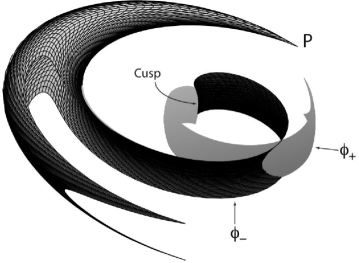
Fig. 3: The bifurcation surface of the observation point P for a source whose rotational motion is counterclockwise. The source points that lie inside this surface influence the field at P at three distinct values of the retarded time, while those that lie outside this surface influence the field at only a single value of the retarded time. The source elements on the filamentary locus at which the cusp curve of this surface intersects the source distribution approach P with the speed of light and zero acceleration at the retarded time and so generate a nonspherically decaying field at P.

The locus of source elements that approach an observer ${\rm P}$ with the wave speed and zero acceleration at the retarded time is given by the intersection of the cusp curve of the bifurcation surface of ${\rm P}$ with the volume of the source. This filamentary locus has exactly the same shape as the cusp curve of the envelope [shown in Fig. 4(a)], except that it resides in the space of source points, instead of the space of observation points, and points in the direction of the source velocity. The projection of this curve onto the $(r,z)$ plane consists of a branch of a hyperbola with asymptotes that lie along the angles $\arcsin(\hat{r}_{\rm P}^{-1})$ and $\pi-\arcsin(\hat{r}_{\rm P}^{-1})$ with respect to the $z$ axis [see Fig. 4(b)]. For an observation point that is located in the far zone, therefore, the projection of the cusp curve of the bifurcation surface onto the $(r,z)$ plane is virtually parallel to the rotation axis.

The reciprocity relations referred to above ensure that if a source element ${\rm S}$ is located on the cusp curve of the bifurcation surface of an observer ${\rm P}$, then the envelope of the wave fronts emitted by ${\rm S}$ would have a cusp passing through ${\rm P}$ (or, conversely, if an observer ${\rm P}$ is located on the cusp curve of the envelope of wave fronts emitted by a source element ${\rm S}$, then the cusp curve of the bifurcation surface of ${\rm P}$ would pass through ${\rm S}$). In the case of a single point source, the retarded position $\varphi$ of the source linearly changes with time ($\varphi={\hat{\varphi}}+\omega t$), and so the cusp that it generates is both spiral-shaped and rigidly rotates about the $z$ axis. In the case of an extended source, on the other hand, the position $\varphi$ of each contributing source element (an element that lies on the cusp curve of the bifurcation surface of a far-field observer ${\rm P}$) is fixed ($\varphi=\varphi_{\rm P}+3\pi/2$, $\hat{r}=\csc\theta_{\rm P}$), and the elements that occupy that position are constantly changing. The cusps generated by the moving source elements that pass through this fixed position at various retarded times have a locus, at any given observation time, that is straight and stationary as shown in Fig. 2. In other words, the source elements constituting the filament at $\varphi=\varphi_{\rm P}+3\pi/2$, $\hat{r}=\csc\theta_{\rm P}$, each contribute a quasi-instantaneous ‘pulse’ of nonspherically decaying electromagnetic radiation that in the far field appears to have propagated out along a virtually straight-line locus defined by the angle $\theta_{\rm P}=\arcsin({\hat{r}}^{-1})$.

1.E Objectives and organization of the paper

The objectives of the present paper are as follows (the location of the resolution of each objective is given in brackets):

1. to show that the nonspherical decay of the radiation field that arises from a rotating superluminal source remains in force at all distances from this source independently of the frequency of the radiation (Section 3.D);

2. to specify the dimensions of the filamentary part of the source that makes the main contribution toward the value of the nonspherically decaying field [Eqs. (62)–(63)];

3. to show that the bundle of cusps emanating from this filament delineates a radiation ‘subbeam’ that is nondiffracting in one dimension; that is to say, the width of this beam in the polar direction remains the same at all distances from the source [Fig. 2, Eq. (74)];

4. to clarify how the requirements of conservation of energy are met by the nonspherically decaying radiation: the cross-sectional area of each nondiffracting subbeam increases as $R_{\rm P}$, rather than $R_{\rm P}^{2}$, with the distance $R_{\rm P}$ from the source (Section 4); and

5. to show that the overall radiation beam within which the field decays nonspherically consists, in general, of an incoherent superposition of the coherent nondiffracting subbeams described above (Section 4).

We begin with the mathematical formulation of the problem in Section 2. In Section 3, we show that objectives 1 and 2 can be achieved by replacing the method of stationary phase used in Ref. 13 with the method of steepest descents. [26] By converting the Fourier-type integral over the radial extent of the source to a Laplace-type integral and making use of contour integration, we present an asymptotic analysis for which the large parameter is the distance from the source (in units of the light-cylinder radius $c/\omega$) rather than the radiation frequency. Not only is there no restriction on the range of frequencies for which the emission from a rotating superluminal source decays nonspherically, but the more distant the observation point, the more accurate the asymptotic analysis that predicts this decay rate.

The more poweful asymptotic technique we employ here establishes, moreover, that the transverse dimensions of the filamentary part of the source responsible for the nonspherically decaying field are of the order of $\delta\hat{r}\propto{\hat{R}_{\rm P}}^{-2}$ in the radial direction and $\delta\varphi\propto{\hat{R}_{\rm P}}^{-3}$ in the azimuthal direction (see Section 4). The dimension of this filament in the direction parallel to the rotation axis is of the order of the length scale of the source distribution in that direction.

The corresponding dimensions of the bundle of cusps that emanate from the contributing source elements can be easily inferred from the above dimensions of the filamentary region containing these elements. The cusps occupy a solid angle in the space of observation points whose azimuthal width $\delta\varphi_{\rm P}$ has a constant value (as does a conventional radiation beam) but whose polar width $\delta\theta_{\rm P}$ decreases with the distance $R_{\rm P}$ as $R_{\rm P}^{-1}$. This may be seen by considering a cohort of propagating polarization-current volume elements that are at the same azimuthal angle $\varphi$ and radius $r$ (possessing the same speed $r\omega$) but at differing heights $z$. Each will give rise to a cusp in the far zone that forms the angle $\theta_{\rm P}=\arcsin({\hat{r}}^{-1})$ with the $z$ axis, but starts from a different height at the light cylinder (see Fig. 2). The spatial extent in the direction of increasing $\theta_{\rm P}$ of the composite set of cusps from this cohort of volume elements (the subbeam) will therefore be determined solely by the height $\delta z$ of the region confining the polarization current. Projected onto a direction normal to the line of sight, this will result in a width $w=|\delta z|\sin\theta_{\rm P}$ occupied by the cusps that is independent of the distance $R_{P}$ from the source. (Note that $w$ is a fixed linear width, rather than an angular width.)

Thus, the area $R_{\rm P}^{2}\sin\theta_{\rm P}\delta\theta_{\rm P}\varphi_{\rm P}$ subtended by the bundle of cusps defining this subbeam increases as $R_{\rm P}$, rather than $R_{\rm P}^{2}$, with the distance $R_{\rm P}$ from the source. In order that the flux of energy remain the same across a cross section of the subbeam, therefore, it is essential that the Poynting vector associated with this radiation correspondingly decay as $R_{\rm P}^{-1}$, rather than $R_{\rm P}^{-2}$. This requirement is, of course, met automatically by the radiation that propagates along the nondiffracting subbeam.

For a rotating superluminal source with the radial boundaries $\hat{r}_{<}>1$ and $\hat{r}_{>}>\hat{r}_{<}$, the nonspherically decaying radiation is detectable in the far zone only within the conical shell

$$\arcsin(1/\hat{r}_{>})\leq\theta_{\rm P}\leq\arcsin(1/\hat{r}_{<}).$$ (14)

These limits on $\theta_{\rm P}$ merely reflect the fact that a rigidly rotating extended source with finite radial spread entails a limited range of linear speeds $r\omega$; Eq. (13) shows that a limited range of speeds results in a limited spread in the angular positions of the generated subbeams. The overall beam described by Eq. (14) consists, in general, of a superposition of nondiffracting subbeams with widely differing amplitudes and phases. The individual subbeams (which would be narrower and more distinguishable, the further away is the observer from the source) decay nonspherically, but the incoherence of their phase relationships ensures that the integrated flux of energy associated with their superposition across this finite solid angle remains independent of $R_{\rm P}$.

Having made a preliminary description of the salient features of the analysis, we now embark on the detailed treatment of the problem in Sections 2 to 4. We conclude in Section 5 with some remarks on the applicability of our analysis to numerical calculations of the emission from superluminal sources and to the observational data on the giant pulses received from pulsars.

2 The nonspherically decaying component of the radiation field from a rotating superluminal source

As in Ref. 13, we base our analysis on a polarization current density ${\bf j}=\partial{\bf P}/\partial t$ for which

$$P_{r,\varphi,z}(r,\varphi,z,t)=s_{r,\varphi,z}(r,z)\cos(m\hat{\varphi})\cos(\Omega t),\qquad-\pi<\hat{\varphi}\leq\pi,$$ (15)

with

$$\hat{\varphi}\equiv\varphi-\omega t,$$ (16)

where $P_{r,\varphi,z}$ are the components of the polarization ${\bf P}$ in a cylindrical coordinate system based on the axis of rotation, ${\bf s}(r,z)$ is an arbitrary vector that vanishes outside a finite region of the $(r,z)$ space, and $m$ is a positive integer. For a fixed value of $t$, the azimuthal dependence of the density (15) along each circle of radius $r$ within the source is the same as that of a sinusoidal wave train with the wavelength $2\pi r/m$ whose $m$ cycles fit around the circumference of the circle smoothly. As time elapses, this wave train both propagates around each circle with the velocity $r\omega$ and oscillates in its amplitude with the frequency $\Omega$. This is a generic source: One can construct any distribution with a uniformly rotating pattern, $P_{r,\varphi,z}(r,\hat{\varphi},z)$, by the superposition over $m$ of terms of the form $s_{r,\varphi,z}(r,z,m)\cos(m\hat{\varphi})$.

The electromagnetic fields

$${\bf E}=-{\bf\nabla}_{\rm P}A^{0}-\frac{\partial{\bf A}}{\partial(ct_{\rm P})},\quad{\bf B}={\bf\nabla}_{\rm P}{\bf\times A},$$ (17)

that arise from such a source are given, in the absence of boundaries, by the following classical expression for the retarded four-potential:

$$A^{\mu}({\bf x}_{\rm P},t_{\rm P})=c^{-1}\int{\rm d}^{3}x{\rm d}t\,j^{\mu}({\bf x},t)\delta(t_{\rm P}-t-R/c)/R\quad\mu=0,\cdots,3$$ (18)

Here, $({\bf x}_{\rm P},t_{\rm P})=(r_{\rm P},\varphi_{\rm P},z_{\rm P},t_{\rm P})$ and $({\bf x},t)=(r,\varphi,z,t)$ are the space-time coordinates of the observation point and the source points, respectively, $R$ stands for the magnitude of ${\bf R}\equiv{\bf x}_{\rm P}-{\bf x}$, and $\mu=1,2,3$ designate the spatial components, ${\bf A}$ and ${\bf j}$, of $A^{\mu}$ and $j^{\mu}$ in a Cartesian coordinate system.[1]

In Ref. 13, we first calculated the Liénard-Wiechert field that arises from a circularly moving point source (representing a volume element of an extended source) with a superluminal speed $r\omega>c$, i.e. considered a generalization of the synchrotron radiation to the superluminal regime. We then evaluated the integral representing the retarded field (rather than the retarded potential) of the extended source (15) by superposing the fields generated by the constituent volume elements of this source, i.e. by using the generalization of the synchrotron field as the Green’s function for the problem (see also Ref. 15). In the superluminal regime, this Green’s function has extended singularities, singularities that arise from the constructive intereference of the emitted waves on the envelope of wave fronts and its cusp.

Labeling each element of the extended source (15) by its Lagrangian coordinate $\hat{\varphi}$ and performing the integration with respect to $t$ and $\hat{\varphi}$ (or equivalently $\varphi$ and $\hat{\varphi}$) in the multiple integral implied by Eqs. (15)–(18), we showed in Ref. 13 that the resulting expression for the radiation field ${\bf B}$ (or ${\bf E}$) consists of two parts: a part whose magnitude decays spherically, as $R_{\rm P}^{-1}$, with the distance $R_{\rm P}$ from the source (as in any other conventional radiation field), and another part ${\bf B}^{\rm ns}$, with ${\bf E}^{\rm ns}={\hat{\bf n}}{\bf\times}{\bf B}^{\rm ns}$ whose magnitude decays as $R_{\rm P}^{-1/2}$ within the conical shell described by Eq. (14). (Here, ${\hat{\bf n}}\equiv{\bf R}/R$ is a unit vector in the radiation direction.)

The expression found in Ref. 13 [Eq. (47)] for the nonspherically decaying component of the field within this conical shell, in the far zone, is

$${\bf B}^{\rm ns}\simeq -\textstyle{\frac{4}{3}}{\rm i}\exp[{\rm i}(\Omega/\omega)(\varphi_{\rm P}+3\pi/2)]\sum_{\mu=\mu_{\pm}}\mu\exp(-{\rm i}\mu\hat{\varphi}_{\rm P})$$ (19)

$$\times\sum_{j=1}^{3}\bar{q}_{j}\int_{\Delta\geq 0}\hat{r}{\rm d}\hat{r}\,{\rm d}\hat{z}\,\Delta^{-1/2}{\bf u}_{j}\exp(-{\rm i}\mu\phi_{-}),$$

where

$$\mu_{\pm}\equiv(\Omega/\omega)\pm m,$$ (21)

$$\hat{\varphi}_{\rm P}\equiv\varphi_{\rm P}-\omega t_{\rm P},$$ (22)

$$\bar{q}_{j}\equiv(1\;\quad-{\rm i}\Omega/\omega\quad{\rm i}\Omega/\omega),$$ (23)

and

$${\bf u}_{j}\equiv\left\{\begin{array}[]{c}s_{r}\cos\theta_{\rm P}{\hat{\bf e}}_{\parallel}+s_{\varphi}{\hat{\bf e}}_{\perp}\\ -s_{\varphi}\cos\theta_{\rm P}{\hat{\bf e}}_{\parallel}+s_{r}{\hat{\bf e}}_{\perp}\\ -s_{z}\sin\theta_{\rm P}{\hat{\bf e}}_{\parallel}\end{array}\right\},$$ (27)

with $j=1,2,3$. In the above expression, ${\hat{\bf e}}_{\parallel}\equiv{\hat{\bf e}}_{\varphi_{\rm P}}$ (which is parallel to the plane of rotation) and ${\hat{\bf e}}_{\perp}\equiv{\hat{\bf n}}{\bf\times}{\hat{\bf e}}_{\parallel}$ comprise a pair of unit vectors normal to the radiation direction ${\hat{\bf n}}$. The domain of integration in Eq. (19) consists of the part of the source distribution ${\bf s}(r,z)$ that falls within $\Delta\geq 0$ (see Fig. 4).

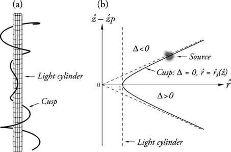
Fig. 4: (a) A segment of the cusp of the envelope of wave fronts emitted by a rotating point source with the speed $r\omega=3c$. This curve is tangent to the light cylinder at the point ($\hat{r}_{\rm P}=1$, $\varphi_{\rm P}=\varphi-3\pi/2$, $\hat{z}_{\rm P}=\hat{z}$) on the plane of the orbit and spirals outward into the far zone. Note that this figure represents a snapshot at a fixed value of the observation time $t_{\rm P}$. The cusp curve of the bifurcation surface of an observer ${\rm P}$ shown in Fig. 3 has precisely the same shape, except that it resides in the space of source points, instead of the space of observation points, and spirals in the counterclockwise direction: It is tangent to the light cylinder at the point ($\hat{r}=1$, $\varphi=\varphi_{\rm P}+3\pi/2$, $\hat{z}=\hat{z}_{\rm P}$). (b) The projections of the cusp curve of the bifurcation surface and a localized source distribution onto the $(\hat{r},\hat{z})$ plane. Only the part of the source that lies close to the cusp in $\Delta>0$ contributes to the nonspherically decaying radiation. The source elements whose $(\hat{r},\hat{z})$ coordinates fall in $\Delta<0$ approach the observer with a speed ${\rm d}R/{\rm d}t<c$ at the retarded time and so make contributions toward the field that are no different from those made in the subluminal regime. The asymptotes of the hyperbola $\Delta=0$ make the angles $\arcsin(1/\hat{r}_{\rm P})$ and $\pi-\arcsin(1/\hat{r}_{\rm P})$ with the $z$ axis, so that for an observation point in the far zone ($\hat{r}_{\rm P}\gg 1$) the projection of the cusp onto the $(\hat{r},\hat{z})$ plane is (as depicted in Fig. 2) effectively parallel to the rotation axis.

The function $\phi_{-}(\hat{r},\hat{z})$ that appears in the phase of the integrand in Eq. (19) is stationary as a function of $\hat{r}$ at

$$\hat{r}=\hat{r}_{\rm C}(\hat{z})\equiv\{\textstyle{\frac{1}{2}}({\hat{r}_{\rm P}}^{2}+1)-[\textstyle{\frac{1}{4}}({\hat{r}_{\rm P}}^{2}-1)^{2}-(\hat{z}-\hat{z}_{\rm P})^{2}]^{1/2}\}^{1/2}.$$ (28)

When the observer is located in the far zone, this isolated stationary point coincides with the locus,

$$\hat{r}=\hat{r}_{\rm S}\equiv[1+(\hat{z}-\hat{z}_{\rm P})^{2}/({\hat{r}_{\rm P}}^{2}-1)]^{1/2},$$ (29)

of source points that approach the observer with the speed of light and zero acceleration at the retarded time, i.e. with the projection of the cusp curve of the bifurcation surface onto the $(r,z)$ plane (see Fig. 4). For $\hat{R}_{\rm P}\gg 1$, the separation $\hat{r}_{\rm C}-\hat{r}_{\rm S}$ vanishes as ${\hat{R}_{\rm P}}^{-2}$ [see Eq. (43) below] and both $\hat{r}_{\rm C}$ and $\hat{r}_{\rm S}$ assume the value $\csc\theta_{\rm P}$.

It follows from Eq. (10) that

$$\phi_{-}|_{\hat{r}=\hat{r}_{\rm C}}\equiv\phi_{\rm C}=\hat{R}_{\rm C}+\varphi_{\rm C}-\varphi_{\rm P},$$ (30)

$\partial\phi_{-}/\partial\hat{r}|_{\hat{r}=\hat{r}_{\rm C}}=0$, and

$$\left.\frac{\partial^{2}\phi_{-}}{\partial\hat{r}^{2}}\right|_{\hat{r}=\hat{r}_{\rm C}}\equiv a=-{\hat{R}_{\rm C}}^{-1}[({\hat{r}_{\rm P}}^{2}-1)({\hat{r}_{\rm C}}^{2}-1)^{-1}-2],$$ (31)

where

$$\varphi_{\rm C}=\varphi_{\rm P}+2\pi-\arccos(\hat{r}_{\rm C}/\hat{r}_{\rm P})$$ (32)

and

$$\hat{R}_{\rm C}=\hat{r}_{\rm C}({\hat{r}_{\rm P}}^{2}-{\hat{r}_{\rm C}}^{2})^{1/2}.$$ (33)

Note that for observation points of interest to us (the observation points located outside the plane of rotation, $\theta_{\rm P}\neq\pi/2$, in the far zone, $\hat{R}_{\rm P}\gg 1$), the parameter $a$ has a value whose magnitude increases with increasing $\hat{R}_{\rm P}$:

$$a\simeq-\hat{R}_{\rm P}\sin^{4}\theta_{\rm P}\sec^{2}\theta_{\rm P}$$ (34)

[see Eq. (31)]. In other words, the phase function $\phi_{-}$ is more peaked at its maximum, the farther the observation point is from the source.

This property of the phase function $\phi_{-}$ distinguishes the asymptotic analysis that will be presented in the following section from those commonly encountered in radiation theory. What turns out to play the role of a large parameter in this asymptotic expansion is distance ($\hat{R}_{\rm P}$), not frequency ($\mu_{\pm}\omega$).

3 Asymptotic analysis of the integral representing the field for large distance

3.A Transformation of the phase of the integrand into a canonical form

The first step in the asymptotic analysis of the integral that appears in Eq. (19) is to introduce a change of variable $\xi=\xi(\hat{r},\hat{z})$ that replaces the original phase $\phi_{-}$ of the integrand by as simple a polynomial as possible. This transformation should be one-to-one and should preserve the number and nature of the stationary points of the phase.[25, 26] Since $\phi_{-}$ has a single isolated stationary point at $\hat{r}=\hat{r}_{\rm C}(\hat{z})$, it can be cast into a canonical form by means of the following transformation:

$$\phi_{-}(\hat{r},\hat{z})=\phi_{\rm C}(\hat{z})+\textstyle{\frac{1}{2}}a(\hat{z})\xi^{2},$$ (35)

in which $a$ is the coefficient given in Eqs. (31) and (34).

The integral in Eq. (19) can thus be written as

$$\int_{\Delta\geq 0}\hat{r}{\rm d}\hat{r}\,{\rm d}\hat{z}\,\Delta^{-1/2}{\bf u}_{j}\exp(-{\rm i}\mu\phi_{-})=\int_{\xi\geq\xi_{\rm S}}{\rm d}\hat{z}{\rm d}\xi\,A(\xi,\hat{z})\exp({\rm i}\alpha\xi^{2}),$$ (36)

in which

$$A(\xi,\hat{z})\equiv\hat{r}\Delta^{-1/2}{\bf u}_{j}\frac{\partial\hat{r}}{\partial\xi}\exp(-{\rm i}\mu\phi_{\rm C}),$$ (37)

with

$$\frac{\partial\hat{r}}{\partial\xi}=a\xi\hat{r}\hat{R}_{-}(\hat{r}^{2}-1-\Delta^{1/2})^{-1},$$ (38)

and $\alpha\equiv-\mu a/2$. The stationary point $\hat{r}=\hat{r}_{\rm C}$ and the boundary point $\hat{r}=\hat{r}_{\rm S}$ respectively map onto $\xi=0$ and

$$\xi=\xi_{\rm S}\equiv-[2a^{-1}(\phi_{\rm S}-\phi_{\rm C})]^{1/2}$$ (39)

where

$$\phi_{\rm S}\equiv\phi_{-}|_{\hat{r}=\hat{r}_{\rm S}}=2\pi-\arccos[1/(\hat{r}_{\rm S}\hat{r}_{\rm P})]+({\hat{r}_{\rm S}}^{2}{\hat{r}_{\rm P}}^{2}-1)^{1/2}.$$ (40)

The upper limit of integration in Eq. (36) is determined by the image of the support of the source density (${\bf s}$ in ${\bf u}_{j}$) under the transformation (35).

The Jacobian $\partial\hat{r}/\partial\xi$ of the above transformation is indeterminate at $\xi=0$. Its value at this critical point has to be found by repeated differentiation of Eq. (35) with respect to $\xi$,

$$\frac{\partial\phi_{-}}{\partial\hat{r}}\frac{\partial\hat{r}}{\partial\xi}=a\xi,$$ (41)

$$\frac{\partial^{2}\phi_{-}}{\partial\hat{r}^{2}}\left(\frac{\partial\hat{r}}{\partial\xi}\right)^{2}+\frac{\partial\phi_{-}}{\partial\hat{r}}\frac{\partial^{2}\hat{r}}{\partial\xi^{2}}=a,$$ (42)

and the evaluation of the resulting relation (42) at $\hat{r}=\hat{r}_{\rm C}$ with the aid of Eq. (31). This procedure, which amounts to applying l’Hôpital’s rule, yields $\partial\hat{r}/\partial\xi|_{\xi=0}=1$: a result that could have been anticipated in light of the coincidence of transformation (35) with the Taylor expansion of $\phi_{-}$ about $\hat{r}=\hat{r}_{\rm C}$ to within the leading order. Correspondingly, the amplitude $A(\xi)$ that appears in Eq. (37) has the value $\hat{r}_{\rm C}({\hat{r}_{\rm C}}^{2}-1)^{-1}{\bf u}_{j}|_{\hat{r}=\hat{r}_{\rm C}}\exp(-{\rm i}\mu\phi_{\rm C})$ at the critical point ${\rm C}$.

When the observer is located in the far field ($\hat{R}_{\rm P}\gg 1$), the phase of the integrand on the right-hand side of Eq. (36) is rapidly oscillating irrespective of how low the harmonic numbers $\mu_{\pm}$ (i.e. the radiation frequencies $\mu_{\pm}\omega$) may be. The leading contribution to the asymptotic value of integral (36) from the stationary point $\xi=0$ can therefore be determined by the method of stationary phase.[25] However, in the limit $\hat{R}_{\rm P}\to\infty$, $\xi_{\rm S}$ reduces to

$$\xi_{\rm S}\simeq-3^{-1/2}\cos^{4}\theta_{\rm P}\csc^{5}\theta_{\rm P}{\hat{R}_{\rm P}}^{-2},$$ (43)

so that the stationary point $\xi=0$ is separated from the boundary point $\xi=\xi_{\rm S}$ by an interval of the order of ${\hat{R}_{\rm P}}^{-2}$ only. To determine the extent of the interval in $\hat{r}$ from which the dominant contribution toward the value of the radiation field arises, we therefore need to employ a more powerful technique for the asymptotic analysis of integral (36), a technique that is capable of handling the contributions from both $\hat{r}_{\rm C}$ and $\hat{r}_{\rm S}$ simultaneously.

3.B Contours of steepest descent

The technique we shall employ for this purpose is the method of steepest descents.[26] We regard the variable of integration in

$$I(\hat{z})\equiv\int_{\xi_{\rm S}}^{\xi_{>}}{\rm d}\xi\,A(\xi,\hat{z})\exp({\rm i}\alpha\xi^{2})$$ (44)

as complex, i.e. write $\xi=u+{\rm i}v$, and invoke Cauchy’s integral theorem to deform the original path of integration into the contours of steepest descent that pass through each of the critical points $\xi=\xi_{\rm S}$, $\xi=0$, and $\xi=\xi_{>}$. Here, we have introduced the real variable $\xi_{>}(\hat{z})$ to designate the image of $\hat{r}_{>}$ under transformation (35), i.e. the boundary of the support of the source term ${\bf u}_{j}$ that appears in the amplitude $A(\xi,\hat{z})$. We shall only treat the case in which $\mu$ (and hence $\alpha$) is positive; $I(\hat{z})$ for negative $\mu$ can then be obtained by taking the complex conjugate of the derived expression and replacing $\phi_{\rm C}$ with $-\phi_{\rm C}$ [see Eq. (37)].

Fig. 5: The integration contours in the complex plane $\xi=u+{\rm i}v$. The critical point ${\rm C}$ lies at the origin, and $u_{\rm S}$ and $u_{>}$ are the images under transformation (35) of the radial boundaries $\hat{r}=\hat{r}_{\rm S}(\hat{z})$ and $\hat{r}=\hat{r}_{>}(\hat{z})$ of the part of the source that lies within $\Delta>0$ (see Fig. 4). The contours $C_{1}$, $C_{2}$, and $C_{3}$ are the paths of steepest descent through the stationary point ${\rm C}$ and the lower and upper boundaries of the integration domain, respectively.

The path of steepest descent through the stationary point ${\rm C}$ at which $\xi=0$ is given, according to

$${\rm i}\xi^{2}=-2uv+{\rm i}(u^{2}-v^{2}),$$ (45)

by $u=v$ when $\alpha$ is positive. If we designate this path by $C_{1}$ (see Fig. 5), then

$$\int_{C_{1}}{\rm d}\xi A(\xi,\hat{z})\exp({\rm i}\alpha\xi^{2})=(1+{\rm i})\int_{-\infty}^{\infty}{\rm d}vA|_{\xi=(1+{\rm i})v}\exp(-2\alpha v^{2})$$ (46)

$$\simeq(2\pi/\mu)^{1/2}\exp[-{\rm i}(\mu\phi_{\rm C}-\pi/4)]{\bf u}_{j}|_{\rm C}\csc\theta_{\rm P}|\sec\theta_{\rm P}|{\hat{R}_{\rm P}}^{-1/2},$$

for $\hat{R}_{\rm P}\gg 1$. Here, we have obtained the leading term in the asymptotic expansion of the above integral for large $\hat{R}_{\rm P}$ by approximating $A|_{\xi=(1+{\rm i})v}$ by its value at ${\rm C}$, where $v=0$, and using Eq. (34) to replace $\alpha$ by its value in the far zone. Note that the next term in this asymptotic expansion is by a factor of order ${\hat{R}_{\rm P}}^{-1/2}$ smaller than this leading term.

The path of steepest descent through the boundary point ${\rm S}$, at which $u\equiv u_{\rm S}=\xi_{\rm S}$ and $v=0$ [see Eqs. (39) and (43)], is given by $u=-(v^{2}+{u_{\rm S}}^{2})^{1/2}$, i.e. by the contour designated as $C_{2}$ in Fig. 5. The real part of

$${\rm i}\xi^{2}|_{C_{2}}=2v(v^{2}+{u_{\rm S}}^{2})^{1/2}+{\rm i}{u_{\rm S}}^{2}$$ (47)

is a monotonic function of $v$ and so can be used as a curve parameter for contour $C_{2}$ in place of $v$. If we let $2v(v^{2}+{u_{\rm S}}^{2})^{1/2}\equiv-\sigma$, then it follows from

$$\xi|_{C_{2}}=-({u_{\rm S}}^{2}+{\rm i}\sigma)^{1/2}$$ (48)

that

$$\int_{C_{2}}{\rm d}\xi A(\xi,\hat{z})\exp({\rm i}\alpha\xi^{2}) = \textstyle{\frac{1}{2}}\exp[{\rm i}(\alpha{u_{\rm S}}^{2}-\pi/2)]$$ (49)

$$\times\int_{0}^{\infty}{\rm d}\sigma\,({u_{\rm S}}^{2}+{\rm i}\sigma)^{-1/2}A\big{|}_{\xi=-({u_{\rm S}}^{2}+{\rm i}\sigma)^{1/2}}\exp(-\alpha\sigma).$$

The function $A|_{C_{2}}$ that here enters the integrand can be determined only by inverting the original transformation (35).

However, since the dominant contribution towards the asymptotic value of the above integral for $\hat{R}_{\rm P}\gg 1$ comes from the vicinity of the boundary point ${\rm S}$, the required inversion of transformation (35) needs to be carried out only to within the leading order in $\sigma$. The Taylor expansions of $\phi_{\pm}(\hat{r},\hat{z})$ about $\hat{r}=\hat{r}_{\rm S}(\hat{z})$ are of the forms

$$\phi_{\pm} = \phi_{\rm S}+{\hat{r}_{\rm S}}^{-1}({\hat{r}_{\rm S}}^{2}-1)({\hat{r}_{\rm S}}^{2}{\hat{r}_{\rm P}}^{2}-1)^{-1/2}(\hat{r}-\hat{r}_{\rm S})$$ (50)

$$\pm\textstyle{\frac{1}{3}}(2\hat{r}_{\rm S})^{3/2}({\hat{r}_{\rm P}}^{2}-1)^{3/2}({\hat{r}_{\rm S}}^{2}{\hat{r}_{\rm P}}^{2}-1)^{-3/2}(\hat{r}-\hat{r}_{\rm S})^{3/2}+\cdots.$$

According to Eqs. (35) and (39), on the other hand,

$$\phi_{-}-\phi_{\rm S}=\textstyle{\frac{1}{2}}a(\xi^{2}-{\xi_{\rm S}}^{2}).$$ (51)

In the vicinity of $\xi=\xi_{\rm S}$, therefore, Eqs. (50) and (51) jointly yield

$$\hat{r}\simeq\hat{r}_{\rm S}+\textstyle{\frac{1}{2}}\sin^{5}\theta_{\rm P}\sec^{4}\theta_{\rm P}{\hat{R}_{\rm P}}^{2}({\xi_{\rm S}}^{2}-\xi^{2})$$ (52)

for $\hat{R}_{\rm P}\gg 1$. Note that ${\xi_{\rm S}}^{2}-\xi^{2}=-{\rm i}\sigma$ and that close to the cusp in the far zone

$$\Delta^{1/2}\simeq(2\sin\theta_{\rm P})^{1/2}\hat{R}_{\rm P}(\hat{r}-\hat{r}_{\rm S})^{1/2},\qquad|\hat{r}-\hat{r}_{\rm S}|\ll 1,\qquad\hat{R}_{\rm P}\gg 1.$$ (53)

Hence, inserting Eqs. (52) and (53) in Eq. (37), taking the limit $\hat{R}_{\rm P}\to\infty$, and expressing $\xi$ in terms of $\sigma$, we find that

$$A|_{C_{2}}\simeq\exp[-{\rm i}(\mu\phi_{\rm C}-\pi/4)]{\bf u}_{j}|_{\rm S}\sin\theta_{\rm P}\sec^{2}\theta_{\rm P}({u_{\rm S}}^{2}+{\rm i}\sigma)^{1/2}\sigma^{-1/2}$$ (54)

in the immediate vicinity of the point ${\rm S}$ at which $\sigma=0$.

Strictly speaking, we should excise the singularity of $A$ at $\sigma=0$ by means of an arc-shaped contour. However, since this singularity is integrable and so has no associated residue, the contribution from such a contour vanishes in the limit that its arc length tends to zero. An alternative way of handling the removeable singularity at $\sigma=0$, followed below, is to introduce a change of integration variable. If we let $\sigma=\tau^{2}$, then the integral in Eq. (49) assumes the form

$$\int_{C_{2}}{\rm d}\xi A(\xi,\hat{z})\exp({\rm i}\alpha\xi^{2}) \simeq \sin\theta_{\rm P}\sec^{2}\theta_{\rm P}\exp[-{\rm i}(\mu\phi_{\rm C}+\pi/4)]{\bf u}_{j}|_{\rm S}\int_{0}^{\infty}{\rm d}\tau\exp(-\alpha\tau^{2})$$ (55)

$$\simeq \textstyle{\frac{1}{2}}(2\pi/\mu)^{1/2}\csc\theta_{\rm P}|\sec\theta_{\rm P}|\exp[-{\rm i}(\mu\phi_{\rm C}+\pi/4)]{\bf u}_{j}|_{\rm S}{\hat{R}_{\rm P}}^{-1/2},$$

where use has been made of Eq. (34) and the definition $\alpha\equiv-\mu a/2$. Note that this differs from the corresponding expression in Eq. (46) for the integral over $C_{1}$ by the factor $\textstyle{\frac{1}{2}}\exp(-{\rm i}\pi/2)$.

The path of steepest descent through the boundary point $\xi=\xi_{>}$, at which $u=u_{>}$, $v=0$, is given by $u=(v^{2}+{u_{>}}^{2})^{1/2}$, i.e. by the contour designated as $C_{3}$ in Fig. 5. The real part of the exponent

$${\rm i}\xi^{2}|_{C_{3}}=-2v(v^{2}+{u_{>}}^{2})^{1/2}+{\rm i}{u_{>}}^{2}$$ (56)

is again a monotonic function of $v$ and so can be used to parametrize contour $C_{3}$ in place of $v$. If we let $2v(v^{2}+{u_{>}}^{2})^{1/2}\equiv\chi$, then it follows from

$$\xi|_{C_{3}}=({u_{>}}^{2}+{\rm i}\chi)^{1/2}$$ (57)

that

$$\int_{C_{3}}{\rm d}\xi A(\xi,\hat{z})\exp({\rm i}\alpha\xi^{2}) = \textstyle{\frac{1}{2}}\exp[{\rm i}(\alpha{u_{>}}^{2}-\pi/2)]$$ (58)

$$\times\int_{0}^{\infty}{\rm d}\chi\,({u_{>}}^{2}+{\rm i}\chi)^{-1/2}A\big{|}_{\xi=({u_{>}}^{2}+{\rm i}\chi)^{1/2}}\exp(-\alpha\chi).$$

The asymptotic value of this integral for $\hat{R}_{\rm P}\gg 1$ receives its dominant contribution from $\chi=0$. Because the function $A|_{C_{3}}$ is regular, on the other hand, its value at $\chi=0$ can be found by simply evaluating the expression in Eq. (37) at $\hat{r}=\hat{r}_{>}$. The result, for $\hat{R}_{\rm P}\to\infty$, is

$$A|_{C_{3},\chi=0}\simeq{\hat{r}_{>}}^{2}\sin^{4}\theta_{\rm P}\sec^{2}\theta_{\rm P}({\hat{r}_{>}}^{2}\sin^{2}\theta_{\rm P}-1)^{-1}{\bf u}_{j}|_{\hat{r}=\hat{r}_{>}}\exp(-{\rm i}\mu\phi_{\rm C})u_{>}$$ (59)

[see Eqs. (8)) and (34)]. This in conjunction with Watson’s lemma therefore implies that

$$\int_{C_{3}}{\rm d}\xi A(\xi,\hat{z})\exp({\rm i}\alpha\xi^{2}) \simeq 2^{1/2}{{\hat{r}}_{>}}^{2}({\hat{r}_{>}}^{2}\sin^{2}\theta_{\rm P}-1)^{-1}{\bf u}_{j}|_{\hat{r}_{>}}$$ (60)

$$\times\exp[-{\rm i}(\mu\phi_{-}|_{\hat{r}_{>}}+\pi/4)]\mu^{-1}{\hat{R}_{\rm P}}^{-1},$$

to within the leading order in ${\hat{R}_{\rm P}}^{-1}$.

3.C Asymptotic value of the radiation field

The integral in Eq. (36) equals the sum of the three contour integrals that appear in Eqs. (46), (55) and (60); the contributions of the contours that connect $C_{1}$ and $C_{2}$, and $C_{1}$ and $C_{3}$, at infinity (see Fig. 5) are exponentially small compared to those of $C_{1}$, $C_{2}$ and $C_{3}$ themselves. On the other hand, the leading term in the asymptotic value of the integral over $C_{3}$ decreases (with increasing $\hat{R}_{\rm P}$) much faster than those of the integrals over $C_{1}$ and $C_{2}$: The integral over $C_{3}$ decays as ${\hat{R}_{\rm P}}^{-1}$, while the integrals over $C_{1}$ and $C_{2}$ decay as ${\hat{R}_{\rm P}}^{-1/2}$ [see Eqs. (46), (55), and (60)]. The leading term in the asymptotic expansion of the radiation field ${\bf B}^{\rm ns}$ for large $\hat{R}_{\rm P}$ is therefore given, according to Eqs. (19), (36), and (46), by

$${\bf B}^{\rm ns} \simeq -\textstyle{\frac{2}{3}}(1+2{\rm i})(2\pi)^{1/2}{\hat{R}_{\rm P}}^{-1/2}|\sec\theta_{\rm P}|\csc\theta_{\rm P}\exp[{\rm i}(\Omega/\omega)(\varphi_{\rm P}+3\pi/2)]\sum_{\mu=\mu_{\pm}}|\mu|^{1/2}$$ (61)

$$\times{\rm sgn}(\mu)\exp({\rm i}\textstyle{\frac{\pi}{4}}{\rm sgn}\,\mu)\sum_{j=1}^{3}\bar{q}_{j}\int_{-\infty}^{\infty}{\rm d}\hat{z}{\bf u}_{j}|_{\rm C}\exp[-{\rm i}\mu(\phi_{\rm C}+\hat{\varphi}_{\rm P})],$$

in which $\mu_{\pm}$ can also be negative (see the first paragraph of Section 3.B).

This result agrees with that in Eq. (55) of Ref. 13. The two expressions differ by a factor of $2-{\rm i}$ because we have here included the additional contribution that arises from the source elements in the (vanishingly small) interval $\hat{r}_{\rm S}\leq\hat{r}\leq\hat{r}_{\rm C}$. The integration with respect to $\hat{r}$ in Eq. (52) of Ref. 13 extends over $\hat{r}_{\rm C}\leq\hat{r}\leq\hat{r}_{>}$, while that in Eq. (44) extends over $\hat{r}_{\rm S}\leq\hat{r}\leq\hat{r}_{>}$. The contribution from $\hat{r}_{\rm S}\leq\hat{r}\leq\hat{r}_{\rm C}$ is given, according to Cauchy’s theorem, by the contribution from the lower half of $C_{1}$ plus the contribution from $C_{2}$.

Even though the length of the interval $\hat{r}_{\rm S}\leq\hat{r}\leq\hat{r}_{\rm C}$ vanishes as ${\hat{R}_{\rm P}}^{-2}$ as $\hat{R}_{\rm P}$ tends to infinity [see Eq. (43)], the contribution that arises from this interval towards the value of the field has the same order of magnitude as that which arises from $\hat{r}_{\rm C}\leq\hat{r}\leq{\hat{r}}_{>}$, and is by a factor of order ${\hat{R}_{\rm P}}^{1/2}$ greater than that which arises from the open interval $\hat{r}_{\rm C}<\hat{r}\leq{\hat{r}}_{>}$. Thus, the nonspherically decaying component of the radiation field that is observed at any given $({\bf x}_{\rm P},t_{\rm P})$ arises from those elements of the source, located at the intersection of the cusp curve of the bifurcation surface with the volume of the source (Fig. 4), that occupy the vanishingly small radial interval

$$\delta\hat{r}\equiv\hat{r}_{\rm C}-\hat{r}_{\rm S}\simeq\textstyle{\frac{1}{2}}\cos^{4}\theta_{\rm P}\csc^{5}\theta_{\rm P}{\hat{R}_{\rm P}}^{-2}$$ (62)

adjacent to the cusp at $\hat{r}=\hat{r}_{\rm S}\simeq\csc\theta_{\rm P}$ [see Eqs. (28) and (29)].

The corresponding azimuthal extent of the source from which the contribution described by Eq. (19) arises is given by the separation $\phi_{+}-\phi_{-}$ of the two sheets of the bifurcation surface shown in Fig. 3 close to the cusp curve of this surface: The contribution of the source elements outside the bifurcation surface is by a factor of the order of $\hat{R}_{\rm P}^{-1/2}$ smaller than those of the elements close to the cusp inside this surface [see Eqs. (41) and (42) of Ref. 13]. Since $\phi_{+}-\phi_{-}\simeq(2^{5/2}/3)(\csc\theta_{\rm P})^{-3/2}(\hat{r}-\hat{r}_{\rm S})^{3/2}$ for $|\hat{r}-\hat{r}_{\rm S}|\ll 1$ and $\hat{R}_{\rm P}\gg 1$ [see Eq. (50)], and the contributing interval in $\hat{r}$ is of the order of ${\hat{R}_{\rm P}}^{-2}$ [see Eq. (62)], it follows that the contributing interval in $\varphi$ is

$$\delta\varphi\equiv(\phi_{+}-\phi_{-})_{\hat{r}=\hat{r}_{\rm C}}\simeq\textstyle{\frac{2}{3}}\cot^{6}\theta_{\rm P}{\hat{R}_{\rm P}}^{-3}.$$ (63)

The contribution from this vanishingly small azimuthal extent of the rotating source is made when the retarded position of this part of the source is $\varphi=\varphi_{\rm C}$ [see Eq. (32)], i.e. when the contributing source elements approach the observer with the speed of light and zero acceleration along the radiation direction. Thus, the source that generates the nonspherically decaying field observed at a point $(\hat{R}_{\rm P},\theta_{\rm P},\varphi_{\rm P})$ in the far zone ($\hat{R}_{\rm P}\gg 1$) consists entirely of the narrow filament parallel to the $z$ axis that occupies a radial interval $\delta\hat{r}\propto{\hat{R}_{\rm P}}^{-2}$ encompassing $\hat{r}\simeq\csc\theta_{\rm P}$ and an azimuthal interval $\delta\varphi\propto{\hat{R}_{\rm P}}^{-3}$ encompassing $\varphi\simeq\varphi_{\rm P}+3\pi/2$ at the retarded time.

3.D Frequency independence of the nonspherical decay

A further implication of the above analysis is that the generated field decays nonspherically irrespective of what the values of the frequencies $\mu_{\pm}\omega$ may be. There is no approximation involved in introducing the transformation (35), and the asymptotic expansion is for large $\alpha$. As derived here, therefore, the only condition for the validity of Eq. (61) is that the absolute value of $\alpha\simeq\frac{1}{2}\mu_{\pm}\hat{R}_{\rm P}\sin^{4}\theta_{\rm P}\sec^{2}\theta_{\rm P}$ should be large, a condition that is automatically satisfied in the far zone for all nonzero frequencies.

That the leading term in the asymptotic expansion of the integral in Eq. (36) is proportional to ${\hat{R}_{\rm P}}^{-1/2}$, instead of ${\hat{R}_{\rm P}}^{-1}$, is a consequence of the particular features of the phase function $\phi_{-}$ described by Eqs. (30)–(34). These features originate in and reflect the particular properties of the time-domain phase $t+R(t)/c$; they are totally independent of both the wavelength of the radiation and the size of the source. In contrast to all other nonspherically decaying solutions of Maxwell’s equations reported in the published literature (see, e.g., Refs. 27, 28, 29), whose slow spreading and decay only occur within the Fresnel distance from the source, the nonspherical decay that is discussed here remains in force at all distances. In fact, the greater the distance $R_{\rm P}$ from the source, the more the leading term dominates the asymptotic approximation in Eq. (61).

The remaining $\hat{z}$ integration in the above expression for ${\bf B}^{\rm ns}$ amounts to a Fourier decomposition of the source densities $s_{r,\varphi,z}|_{\rm C}$ with respect to $\hat{z}$. Using Eqs. (30)–(33) to replace $\phi_{\rm C}$ in Eq. (61) by its far-field value

$$\phi_{\rm C}\simeq\hat{R}_{\rm P}-\hat{z}\cos\theta_{\rm P}+3\pi/2,$$ (64)

and using Eq. (27) to write out ${\bf u}_{j}$ in terms of $s_{r,\varphi,z}$, we find that the electric field ${\bf E}^{\rm ns}={\hat{\bf n}}{\bf\times B}^{\rm ns}$ of the nonspherically decaying radiation is given by

$${\bf E}^{\rm ns} \simeq \textstyle{\frac{4}{3}}(2\pi)^{1/2}{\hat{R}_{\rm P}}^{-1/2}|\sec\theta_{\rm P}|\csc\theta_{\rm P}\exp[{\rm i}(\Omega/\omega)(\varphi_{\rm P}+3\pi/2)]\sum_{\mu=\mu_{\pm}}|\mu|^{1/2}$$ (65)

$$\times{\rm sgn}(\mu)\exp({\rm i}\textstyle{\frac{\pi}{4}}{\rm sgn}\,\mu)\exp[-{\rm i}\mu(\hat{R}_{\rm P}+\hat{\varphi}_{\rm P}+3\pi/2)]\{({\rm i}\bar{s}_{\varphi}+\Omega\bar{s}_{r}/\omega){\hat{\bf e}}_{\parallel}$$

$$-[({\rm i}\bar{s}_{r}-\Omega\bar{s}_{\varphi}/\omega)\cos\theta_{\rm P}+\Omega\bar{s}_{z}\sin\theta_{\rm P}/\omega]{\hat{\bf e}}_{\perp}\},$$

in which $\bar{s}_{r,\varphi,z}$ stand for the following Fourier transforms of $s_{r,\varphi,z}|_{\rm C}$ with respect to $\hat{z}$:

$$\bar{s}_{r,\varphi,z}\equiv\int_{-\infty}^{\infty}{\rm d}\hat{z}\,s_{r,\varphi,z}(\hat{r},\hat{z})\big{|}_{\hat{r}=\csc\theta_{\rm P}}\exp({\rm i}\mu\hat{z}\cos\theta_{\rm P}).$$ (66)

This field is observable only at those polar angles $\theta_{\rm P}$ within the interval $\arccos(1/\hat{r}_{<})\leq|\theta_{\rm P}-\pi/2|\leq\arccos(1/\hat{r}_{>})$ for which $s_{r,\varphi,z}|_{\hat{r}=\csc\theta_{\rm P}}$ are nonzero, i.e. at those observation points (outside the plane of rotation) the cusp curve of whose bifurcation surface (Fig. 3) intersects the source distribution (Fig. 4).

3.E Relevance to computational models of the emission from superluminal sources

The asymptotic analysis outlined in this section provides a basis also for the computational treatment of the nonspherically decaying field ${\bf B}^{\rm ns}$. The original formulation of ${\bf B}^{\rm ns}$ appearing in Eq. (19), in which the integral has a rapidly oscillating kernel, is not suitable for computing a field whose value in the radiation zone receives its main contribution from such small fractions of the $\hat{r}$ and $\hat{\varphi}$ integration domains as $\delta\hat{r}\propto{\hat{R}_{\rm P}}^{-2}$ and $\delta\varphi\propto{\hat{R}_{\rm P}}^{-3}$. The above conversion of the Fourier-type integrals to Laplace-type integrals renders the selecting out and handling of the contributions from integrands with such narrow supports numerically more feasible.

4 The collection of nondiffracting subbeams delineating the overall distribution of the nonspherically decaying radiation

We have seen that the wave fronts that emanate from a given volume element of a rotating superluminal source possess an envelope consisting of two sheets that meet along a cusp (Fig. 1). There is a higher-order focusing involved in the generation of the cusp than in that of the envelope itself, so that the intensity of the radiation from an extended source attains its maximum on the bundle of cusps that are emitted by various source elements. If a source element approaches an observeration point ${\rm P}$ with the speed of light and zero acceleration along the radiation direction, then the cusp it generates passes through ${\rm P}$. The reason is that both the locus of source elements that approach the observer with the speed of light and zero acceleration [i.e. the cusp curve of the bifurcation surface (Fig. 3)] and the cusp that is generated by a given source element are described by the same equation: The cusp curve of the bifurcation surface resides in the space of source points and so is given by Eq. (12) for a fixed $(\hat{r}_{\rm P},\varphi_{\rm P},\hat{z}_{\rm P})$, while the cusp curve of the envelope resides in the space of observation points and is given by Eq. (12) for a fixed $(r,\varphi,z)$.

4.A Angular extent of the nonspherically decaying emission

The collection of cusp curves that are generated by the constituent volume elements of an extended source thus defines what might loosely be termed a ‘radiation beam’, although its characteristics are distinct from those of conventionally produced beams. The field decays nonspherically only along the bundle of cusp curves embodying this radiation beam. Since the cusp that is generated by a source element with the radial coordinate $\hat{r}$ lies on the cone $\theta_{\rm P}=\arcsin(1/\hat{r})$ in the far zone, the nonspherically decaying radiation that arises from a source distribution with the radial extent $\hat{r}_{<}\leq\hat{r}\leq\hat{r}_{>}$ is detectable only within the conical shell $\arcsin(1/\hat{r}_{>})\leq\theta_{\rm P}\leq\arcsin(1/\hat{r}_{<})$.

The field that is detected at a given point ${\rm P}$ within this conical shell arises almost exclusively from a filamentary part of the source parallel to the $z$ axis whose radial and azimuthal extents are of the order of $\delta\hat{r}\propto{\hat{R}_{\rm P}}^{-2}$ and $\delta\varphi\propto{\hat{R}_{\rm P}}^{-3}$, respectively [see Eqs. (62) and (63)]. The bundle of cusps emanating from this narrow filament occupies a much smaller solid angle than that described above. The parametric equation $\hat{z}_{\rm P}=\hat{z}_{\rm P}(\hat{r}_{\rm P})$, $\varphi_{\rm P}=\varphi_{\rm P}(\hat{r}_{\rm P})$ of the particular cusp curve that emanates from a given source element $(r,\hat{\varphi},z)$ can be written, using Eq. (12), as

$$\hat{z}_{\rm P}=\hat{z}\pm({\hat{r}_{\rm P}}^{2}-1)^{1/2}(\hat{r}^{2}-1)^{1/2},$$ (67)

$$\varphi_{\rm P}=\varphi-2\pi+\arccos[1/(\hat{r}\hat{r}_{\rm P})].$$ (68)

If we rewrite Eqs. (67) and (68) in terms of the spherical polar coordinates $(R_{\rm P},\theta_{\rm P},\varphi_{\rm P})$ of the observation point ${\rm P}$ and solve them for $\theta_{\rm P}$ and $\varphi_{\rm P}$ as functions of $(r,z)$ and $R_{\rm P}$, we find that the cusp that is generated by a source point with the coordinates $(r,\hat{\varphi},z)$ passes through the following two points on a sphere of radius $R_{\rm P}$:

$$\theta_{\rm P}=\arccos\left\{\frac{1}{\hat{r}\hat{R}_{\rm P}}\left[\frac{\hat{z}}{\hat{r}}\pm(\hat{r}^{2}-1)^{1/2}\left(\hat{R}_{\rm P}^{2}-1-\frac{\hat{z}^{2}}{\hat{r}^{2}}\right)^{1/2}\right]\right\},$$ (69)

and

$$\varphi_{\rm P}=\varphi-2\pi+\arccos[1/(\hat{R}_{\rm P}\hat{r}\sin\theta_{\rm P})],$$ (70)

where the $\pm$ correspond to the two halves of this cusp curve above and below the plane of rotation (see Fig. 4).

The Taylor expansion of the expressions on the right-hand sides of Eqs. (69) and (70) in powers of ${\hat{R}_{\rm P}}^{-1}$ yields

$$\theta_{\rm P}=\arcsin(1/\hat{r})-(\hat{z}/\hat{r}){\hat{R}_{\rm P}}^{-1}\pm\textstyle{\frac{1}{2}}(\hat{r}^{2}-1)^{1/2}{\hat{R}_{\rm P}}^{-2}+\cdots,$$ (71)

and

$$\varphi_{\rm P}=\varphi-3\pi/2-{\hat{R}_{\rm P}}^{-1}+\cdots.$$ (72)

These show that incremental changes $\delta r$, $\delta z$ and $\delta\varphi$ in the position of the source element $(r,\hat{\varphi},z)$ result in the following changes in the $(\theta_{\rm P},\varphi_{\rm P})$ coordinates of the point at which the cusp arising from that element intersects a sphere of radius $R_{\rm P}$ in the far zone:

$$\delta\theta_{\rm P}=-\hat{r}^{-1}(\hat{r}^{2}-1)^{-1/2}\delta\hat{r}-\hat{r}^{-1}\delta\hat{z}{\hat{R}_{\rm P}}^{-1}+\cdots,$$ (73)

and $\delta\varphi_{\rm P}=\delta\varphi+\cdots$. Because $\delta\hat{r}$ is of the order of ${\hat{R}_{\rm P}}^{-2}$, while $\delta\hat{z}$ is of the order of unity for the filamentary source of the field that is detected at ${\rm P}$, the dominant term in the expression on the right-hand side of Eq. (73) is that proportional to the $\hat{z}$ extent of the filament. Given the observation point ${\rm P}$, and hence a set of fixed values for the dimensions ($\delta\hat{r}$, $\delta\varphi$, $\delta\hat{z}$) of the filamentary source of the field that is detected at ${\rm P}$, it therefore follows that the bundle of cusps generated by such a filament occupies a solid angle with the dimensions

$$\delta\theta_{\rm P}\simeq-\delta\hat{z}\sin\theta_{\rm P}{\hat{R}_{\rm P}}^{-1}\quad{\rm and}\quad\delta\varphi_{\rm P}\simeq\delta\varphi$$ (74)

in the far zone. [Here, we have made use of the fact that $\theta_{\rm P}\simeq\arcsin(1/\hat{r})$ to within the zeroth order in ${\hat{R}_{\rm P}}^{-1}$ to express $\hat{r}$ in Eq. (74) in terms of $\theta_{\rm P}$.]

The bundle of cusp curves occupying the solid angle (74) embodies a subbeam that does not diverge in the direction of $\theta_{\rm P}$. The polar width $\delta\theta_{\rm P}$ of this subbeam decreases with the distance $\hat{R}_{\rm P}$ in such a way that the thickness $\hat{R}_{\rm P}\delta\theta_{\rm P}$ of the subbeam in the polar direction remains constant: It equals the projection of the $\hat{z}$ extent, $\delta\hat{z}$, of the contributing filamentary source onto a direction normal to the line of sight at all $\hat{R}_{\rm P}$. The azimuthal width of the subbeam, on the other hand, diverges as does any other radiation beam: $\delta\varphi_{\rm P}$ is independent of $\hat{R}_{\rm P}$ (see Fig. 2).

Thus, the bundle of cusps that emanates from the filamentary locus of the set of source elements responsible for the nonspherically decaying field at ${\rm P}$ intersects a large sphere of radius $R_{\rm P}$ (enclosing the source) along a strip the thickness of whose narrow side is independent of $R_{\rm P}$. According to Eq. (74), the area $R_{\rm P}^{2}\sin\theta_{\rm P}\delta\theta_{\rm P}\delta\varphi_{\rm P}$ subtended by this subbeam increases as $R_{\rm P}$, rather than $R_{\rm P}^{2}$, with the radius of the sphere enclosing the source. Conservation of energy demands, therefore, that the Poynting vector associated with this radiation should correspondingly decrease as $R_{\rm P}^{-1}$ instead of $R_{\rm P}^{-2}$, in order that the flux of energy remain the same across various cross sections of the subbeam. This requirement is, of course, automatically met by the (nonspherical) rate of decay of the intensity of the radiation that propagates along the subbeam.

The nondiffracting subbeams that are detected at two distinct observation points within the solid angle $\arcsin(1/\hat{r}_{>})\leq\theta_{\rm P}\leq\arcsin(1/\hat{r}_{<})$ arise from two distinct filamentary parts of the source with essentially no common elements [see Eqs. (62) and (63)]. The subbeam that passes through an observation point ${\rm P}^{\prime}$, though sharing the same general properties as that which passes through ${\rm P}$, arises from those elements of the source, located at $\hat{r}^{\prime}=\csc\theta_{\rm P^{\prime}}$, $\varphi^{\prime}=\varphi_{\rm P^{\prime}}$, that approach ${\rm P}^{\prime}$, rather than ${\rm P}$, with the speed of light and zero acceleration at the retarded time. Not only are the focused wave packets that embody the cusp constantly dispersed and reconstructed out of other (spherically spreading) waves,[9] but also the filaments that act as sources of these focused waves each occupy a vanishingly small ($\sim{\hat{R}_{\rm P}}^{-5}$) disjoint volume of the overall source distribution, and so are essentially independent of one another. Unlike conventional radiation beams, which have fixed sources, the subbeam that passes through an observation point ${\rm P}$ arises from a source whose location and extent depend on ${\rm P}$.

It would be possible to identify the individual nondiffracting subbeams only in the case of a source whose length scale of spatial variations is comparable to ${\hat{R}_{\rm P}}^{-2}$ (e.g. in the case of a turbulent plasma with a superluminally rotating macroscopic distribution). The overall beam within which the nonspherically decaying radiation is detectable would then consist of an incoherent superposition of coherent, nondiffracting subbeams with widely differing amplitudes and phases. The individual coherent subbeams decay nonspherically, but the incoherence of their phase relationships ensures that the integrated flux of energy associated with their superposition across this finite solid angle remains independent of $R_{\rm P}$. Note that the individual subbeams constituting the overall beam would be narrower and more distinguishable, the farther the observer is from the source.

5 Concluding remarks

The analysis we have presented here was motivated by questions encountered in the course of the design, construction, and testing of practical machines for investigating the emission from superluminal sources.[6] The original mathematical treatment of the nonspherically decaying radiation,[13] in which the integral over the volume of the source has a rapidly oscillating kernel, is not suitable for the computational modeling of the emission from such machines. We have seen that the nonspherically decaying radiation detected in the radiation zone receives its main contribution from such small fractions of the radial and azimuthal integration domains as $\delta\hat{r}\sim{\hat{R}_{\rm P}}^{-2}$ and $\delta\varphi\sim{\hat{R}_{\rm P}}^{-3}$. The above conversion of the Fourier-type integrals to Laplace-type integrals renders the selecting out and handling of the contributions from integrands with such narrow supports numerically more feasible.

Not only the nonspherical decay of its intensity, but also the narrowness of both the beam into which it propagates and the region of the source from which it arises are features that are unique to the emission from a rotating superluminal source. These features are not shared by any other known emission mechanism. On the other hand, they are remarkably similar to the observed features of an emission that has long been known to radio astronomers: to the (as yet unexplained) extreme properties of the giant pulses that are received from pulsars (see, e.g. Refs. 16, 17, 18, 19, 20). The giant radio pulses from the Crab pulsar have a temporal structure of the order of a nanosecond.[18] Under the assumption that they decay spherically like other conventional emissions, the observed values of these pulses’ fluxes imply that their energy densities generally exceed the energy densities of both the magnetic field and the plasma in the magnetosphere of a pulsar by many orders of magnitude.[19] “The plasma structures responsible for these emissions must be smaller than one metre in size, making them by far the smallest objects ever detected and resolved outside the Solar System, and the brightest transient radio sources in the sky.”[18]

The highly stable periodicity of the mean profiles of the observed pulses,[16] i.e. the rigidly rotating distribution of the radiation from pulsars, can only arise from a source whose distribution pattern correspondingly rotates rigidly, a source whose average density depends on the azimuthal angle $\varphi$ in the combination $\varphi-\omega t$ only: Maxwell’s equations demand that the charge and current densities that give rise to this radiation should have exactly the same symmetry ($\partial/\partial t=-\omega\partial/\partial\varphi$) as that of the observed radiation fields ${\bf E}$ and ${\bf B}$. On the other hand, the domain of applicability of such a symmetry casnnot be localized; a solution of Maxwell’s equations that satisfies this symmetry applies either to the entire magnetosphere or to a region whose boundary is an expanding wave front. Unless there is no plasma outside the light cylinder, therefore, the macroscopic distribution of electric current in the magnetosphere of a pulsar should have a superlumially rotating pattern in $r>c/\omega$. The superluminal source described by Eq. (15) captures the essential features of the macroscopic charge-current distribution that is present in the magnetosphere of a pulsar and is thus an inevitable implication of the observational data on these objects.

Once it is acknowledged that the source of the observed giant pulses should have a superluminally rotating distribution pattern, the extreme values of their brightness temperature ($\sim 10^{39}$ ^∘K), temporal width ($\sim 1$ ns), and source dimension ($\sim 1$ m) are all explained by the results of the above analysis. The nonspherical decay of the resulting radiation would imply that the energy density and so the brightness temperature of the observed pulses are by a factor of the order of $\hat{R}/(\hat{r}_{>}-\hat{r}_{<})^{2}$ smaller than those that are normally estimated by using an inverse-square law,[13] a factor that ranges from $10^{15}$ to $10^{25}$ in the case of known pulsars.[16]

The nondiffracting nature of this nonspherically decaying radiation [Eq. (74)], together with its arising only from the filamentary part of the source that approaches the observer with the speed of light and zero acceleration [Eqs. (62) and (63)], likewise explain the values of its temporal width and source dimension. Furthermore, that the overall beam within which the nonspherically decaying radiation is detectable should in general consist of an incoherent superposition of coherent, nondiffracting subbeams (Section 4) is consistent with the conclusion reached by Popov et al.[20] that “the radio emission of the Crab pulsar at the longitudes of the main pulse and interpulse consists entirely of giant pulses.”[20]

Two other features of the emission from a rotating superluminal source that were derived elsewhere[12, 30] are also consistent with the observational data on pulsars:[16] the occurrence of concurrent ‘orthogonal’ polarization modes with swinging position angles[12] and a broadband frequency spectrum.[30]

References

- [1] J. D. Jackson, Classical Electrodynamics, 3rd ed. (Wiley, New York, 1999).
- [2] B. M. Bolotovskii and V. L. Ginzburg, “The Vavilov-Čerenkov effect and the Doppler effect in the motion of sources with superluminal velocity in vacuum,” Sov. Phys. Usp. 15(2), 184–192 (1972).
- [3] V. L. Ginzburg, “Vavilov-Čerenkov effect and anomalous Doppler effect in a medium in which wave phase velocity exceeds velocity of light in vacuum,” Sov. Phys. JETP 35(1), 92–93 (1972).
- [4] B. M. Bolotovskii and V. P. Bykov, “Radiation by charges moving faster than light,” Sov. Phys. Usp. 33(6), 477–487 (1990).
- [5] A. V. Bessarab, A. A. Gorbunov, S. P. Martynenko, and N. A. Prudkoy, “Faster-than-light EMP source initiated by short X-ray pulse of laser plasma,” IEEE Trans. Plasma Sci. 32(3), 1400–1403 (2004).
- [6] A. Ardavan, W. Hayes, J. Singleton, H. Ardavan, J. Fopma, and D. Halliday, “Experimental observation of nonspherically-decaying radiation from a rotating superluminal source,” J. Appl. Phys. 96(12), 7760–7777(E) (2004). Corrected version of 96(8), 4614–4631.
- [7] J. Singleton, A. Ardavan, H. Ardavan, J. Fopma, D. Halliday, and W. Hayes, “Experimental demonstration of emission from a superluminal polarization current—a new class of solid-state source for MHz-THz and beyond,” in Digest of the 2004 Joint 29th International Conference on Infrared and Millimeter Waves and 12th International Conference on Terahertz Electronics (Institute of Electrical and Electronics Engineers, New York, 2004).
- [8] B. M. Bolotovskii and A. V. Serov, “Radiation of superluminal sources in empty space,” Phys. Usp. 48(9), 903–915 (2005).
- [9] H. Ardavan, “Generation of focused, nonspherically decaying pulses of electromagnetic radiation,” Phys. Rev. E 58(5), 6659–84 (1998).
- [10] A. Ardavan and H. Ardavan, “Apparatus for generating focused electromagnetic radiation,” International patent application PCT-GB99-02943 (1999).
- [11] H. Ardavan, “The superluminal model of pulsars,” in Pulsar Astronomy—2000 and Beyond, M. Kramer, N. Wex, and Wielebinski, eds., vol. 202 of Astronomical Society of the Pacific Conference Series, pp. 365–366 (USA: Astron. Soc. Pacific, 2000).
- [12] A. Schmidt, H. Ardavan, J. Fasel, J. Singleton, and A. Ardavan, “Occurrence of concurrent ‘orthogonal’ polarization modes in the Liénard-Wiechert field of a rotating superluminal source,” in Proc. 363rd WE-Heraeus Seminar on Neutron Stars and Pulsars, W. Becker and H. H. Huang, eds., pp. 124–127 (2006). ArXiv: astro-ph/0701257.
- [13] H. Ardavan, A. Ardavan, and J. Singleton, “Spectral and polarization characteristics of the nonspherically decaying radiation generated by polarization currents with superluminally rotating distribution patterns,” J. Opt. Soc. Am. A 21(5), 858–872 (2004).
- [14] J. H. Hannay, “Spectral and polarization characteristics of the nonspherically decaying radiation generated by polarization currents with superluminally rotating distribution patterns: comment,” J. Opt. Soc. Am. A 23(6), 1530–1534 (2006).
- [15] H. Ardavan, A. Ardavan, and J. Singleton, “Spectral and polarization characteristics of the nonspherically decaying radiation generated by polarization currents with superluminally rotating distribution patterns: reply to comment,” J. Opt. Soc. Am. A 23(6), 1535–1539 (2006).
- [16] D. Lorimer and M. Kramer, Handbook of Pulsar Astronomy (Cambridge U. Press, Cambridge, U.K, 2005).
- [17] S. Sallmen, D. C. Backer, T. H. Hankins, D. Moffett, and S. Lundgren, “Simultaneous dual-frequency observations of giant pulses from the Crab pulsar,” Astrophys. J. 517(1), 460–471 (1999).
- [18] T. H. Hankins, J. S. Kern, J. C. Weatherall, and J. A. Eilek, “Nanosecond radio bursts from strong plasma turbulence in the Crab pulsar,” Nature (London) 422(6928), 141–3 (2003).
- [19] V. A. Soglasnov, M. V. Popov, N. Bartel, W. Cannon, A. Y. Novikov, V. I. Kondratiev, and V. I. Altunin, “Giant pulses from PSR B1937+21 with widths nanoseconds and K, the highest brightness temperature observed in the universe,” Astrophys. J. 616(1), 439–451 (2004).
- [20] M. V. Popov, V. A. Soglasnov, V. I. Kondrat’ev, S. V. Kostyuk, and Y. P. Ilyasov, “Giant pulses—The main component of the radio emission of the Crab pulsar,” Atronom. Rep. 50(1), 55–61 (2006).
- [21] G. M. Lilley, R. Westley, A. H. Yates, and Y. R. Busing, “Some aspects of noise from supersonic aircraft,” J. Aeronaut.Soc. 57(510), 396–414 (1953).
- [22] M. V. Lowson, “Focusing of helicopter BVI noise,” J. Sound and Vibration 190(3), 477–94 (1996).
- [23] J. Hadamard, Lectures on Cauchy’s Problem in Linear Partial Differential Equations (Yale University Press, New Haven, 1923). Dover reprint, 1952.
- [24] R. F. Hoskins, Generalized Functions, chap. 7 (Harwood, London, 1979).
- [25] V. A. Borovikov, Uniform Stationary Phase Method (Institution of Electrical Engineers, Stevenage, U.K, 1994).
- [26] N. Bleistein and R. A. Handelsman, Asymptotic Expansions of Integrals (Dover, New York, 1986).
- [27] A. M. Shaarawi, I. M. Besieris, R. W. Ziolkowski, and S. M. Sedky, “Generation of approximate focus-wave-mode pulses from wide-band dynamic Gaussian apertures,” J. Opt. Soc. Am. 12(9), 1954–1964 (1995).
- [28] K. Reivelt and P. Saari, “Experimental demonstration of realizability of optical focus wave modes,” Phys. Rev. E 66(52), 056,611/1–056,611/9 (2002).
- [29] E. Recami, M. Zamboni-Rached, K. Z. Nobrega, C. A. Dartora, and H. E. Hernandez, “On the localized superluminal solutions to the Maxwell equations,” IEEE J. Sel. Top. Quantum Electron. 9(1), 59–73 (2003).
- [30] H. Ardavan, A. Ardavan, and J. Singleton, “Frequency spectrum of focused broadband pulses of electromagnetic radiation generated by polarization currents with superluminally rotating distribution patterns,” J. Opt. Soc. Am. A 20(11), 2137–2155 (2003).