Market reaction to temporary liquidity crises and the permanent market impact

Abstract

We study the relaxation dynamics of the bid-ask spread and of the midprice after a sudden, large variation of the spread, corresponding to a temporary crisis of liquidity in a double auction financial market. We find that the spread decays very slowly to its normal value as a consequence of the strategic limit order placement of liquidity providers. We consider several quantities, such as order placement rates and distribution, that affect the decay of the spread. We measure the permanent impact both of a generic event altering the spread and of a single transaction and we find an approximately linear relation between immediate and permanent impact in both cases.

I Introduction

Many theoretical and empirical studies have examined microstructure properties of double auction financial markets. Limit order book data provide the maximum amount of information at the lowest aggregation level. Early examples of investigations of order book data can be found in Harris96 ; Hamao95 ; Biais95 . Other examples of investigations using limit order books are the developing of econometric models of limit order execution times Lo02 and the empirical investigation of order aggressiveness and trader’ order submission strategy in an open limit order book Hall06 . These microstructure studies are important both for analysing and modeling the dynamics of the limit order book and in the investigation of determinants of key financial variables such as bid-ask spread Huang97 . Moreover, the statistical regularities observed in these investigations can provide empirical and modeling support or falsify conjectures about the origin of stylized facts observed in financial markets.

One of the best known statistical regularities of financial time series is the fact that the empirical distribution of asset price changes is fat tailed, i.e. there is a higher probability of extreme events than in a Gaussian distribution Mandelbrot63 ; Fama64 ; Officer72 ; Akigiray89 ; Mantegna95 ; Longin96 ; Lux96 ; gopi98 ; Plerou99 . Moreover, there are strong indications that the part of the distribution describing large price changes follows a power-law gopi98 . This is important for financial risk, since it means that large price fluctuations are much more common than one might expect. There have been several conjectures about the origin of fat tails in prices Clark73 ; Gabaix03 . Recently Farmer04 it has been suggested that fluctuations of liquidity, i.e. the market’s ability to absorb new market orders, could be at the origin of large price changes. The proposed mechanism for large price change is the following. Even for the most liquid stocks there can be substantial gaps in the order book, corresponding to a block of adjacent price levels containing no quotes. When such a gap exists next to the best price, a new order can remove the best quote, triggering a large midpoint price change. Thus, the distribution of large price changes merely reflects the distribution of gaps in the limit order book. The market order triggering the trade must have a size at least equal to the opposite best and can therefore be of small size. A market order producing an immediate large price change also creates a temporary large spread. The market then reverts the spread to a normal value as a consequence of the events immediately following the trade. This paper empirically investigates how the market reacts to these temporary liquidity crises and how the spread and the price revert back to normal values.

The presence of large spread poses challenging questions to the traders on the optimal way to trade. When the spread is large liquidity takers have a strong disincentive for submitting market orders given that the cost, the bid-ask spread, is large. Conversely market makers (liquidity providers) trade by placing limit orders and therefore profit of a large spread by selling at the ask price and buying back at the lower bid price. Moreover there is a strong incentive to place limit orders in the spread given that a trader can attain the best position (price) in the book with the highest execution priority. However the optimal order placement inside the spread is a nontrivial problem. Slowly closing the spread by placing a limit order at a price just beating the best by one tick and waiting for a market order would give the best execution price (from the point of view of the trader placing the limit order), but this strategy risks being beaten by limit orders of other traders. After some time the price reaches a ‘normal’ value attractive to market order submitters.

Beside the problem of how to close the spread, a large spread also poses the challenge of establishing the “right” level of the price after the temporary liquidity crisis disappears . This problem is important for all types of traders. Liquidity providers have to decide how to readjust their quotes by taking into account the informed nature of the market order which generated the large spread. On the other hand for liquidity takers market impact is one of the most important costs of trading. When a liquidity taker wishes to submit a large order she usually decides to split it in parts and trade it incrementally. Any transaction of a part of the large order pushes the price in a direction that makes the next transaction more unfavorable for her. Thus liquidity takers wish to minimize the price change due to their own trading and they need to know what the permanent part of their own trading is. In the second part of this paper we investigate empirically the relation between immediate and permanent impact.

Our paper is organized as follow. In Section II we present the data set used to perform our empirical analyses. In Section III we present a graphical representation of the order book that might help to visualize some aspects of the book dynamics. Section IV presents the results we have obtained in our investigation of the bid-ask spread dynamics. The determinants of bid-ask spread decay are discussed in Section V. In Section VI we investigate the permanent impact both of a fluctuation and of a transaction altering the spread. In Section VI we briefly discuss our results and draw some conclusions.

II Data

Our dataset is composed of $71$ highly capitalized stocks traded at the London Stock Exchange. The time period is the whole year 2002. The ticker of the investigated stocks are: SHEL, VOD, GSK, RBS, BP., AZN, LLOY, REL, HSBA, BARC, HBOS, ULVR, BT.A, DGE, AV., PRU, BSY, WPP, RIO, ANL, TSCO, RTR, PSON, STAN, CBRY, BA., BG., BLT, BATS, NGT, AVZ, CPG, AAL, ARM, CNA, CW., RSA, KFI, SPW, SUY, IMT, RB., BZP, LGEN, ICI, MKS, GUS, SSE, DXNS, SHP, ALLD, OOM, BOG, BOC, HG., SCTN, BAA, LOG, RR, SMIN, HNS, GAA, NYA, SGE, WOS, AL., SFW, ISYS, III, BAY, RTO. The order of the tick symbol in the list is fixed by its rank when the stocks are sorted according to the size occupied by the stock in the database. SHEL occupied the largest amount of memory in the database while RTO occupied the smallest memory, among the considered stocks.

The LSE has a dual market structures consisting of a centralized limit order book market and a decentralized bilateral exchange. In London the centralized limit order book market is called the on-book market and the decentralized bilateral exchange is called the off-book market. In 2002 $62\%$ of transactions of LSE stocks occurred in the on-book exchange. In our study we consider only the on-book market. The on-book market is a fully automated electronic exchange. Market participants have the ability to view the entire limit order book at any instant, and to place trading orders and have them entered into the book, executed, or canceled almost instantaneously. The trading day begins and terminates with an auction. For this study, we ignore the opening and closing auctions and analyze only orders placed during the continuous auction period. Moreover, in order to avoid effects near the start and end of the day, we omit the first and last half an hour of trading from the calculation each day. That is we make a time series for each day from 8:30 AM to 4:00 PM and using it we calculate the conditional averages and the unconditional averages and repeat the process for each separate day, without including any time lags across different days. Finally, in most of our analyses, we removed the data of trading occurring on September 20, 2002. This is because on that day anomalous behavior of the spread due to unusual trading was observed as described below.

III Grapical Representation of Order Book as Complex Dynamical System

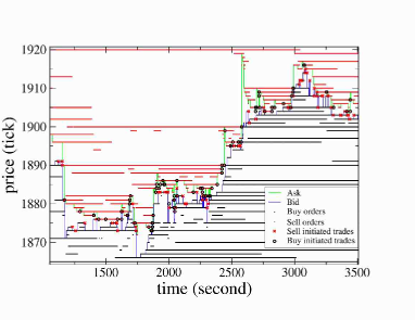
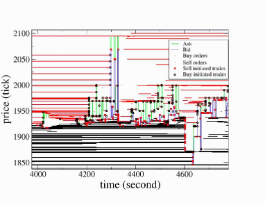
Figure 1: Examples of limit order book time series. Top panel: AZN order book dynamics on September 4, 2002 during normal trading. Time is given in seconds from 8:00 am. Bottom panel: AZN order book dynamics on September 20, 2002 when a rogue trading pattern was occurring. Time is given in seconds from 9:00 am. The plots show all limit order price levels present in the price range shown, as well as the bid (blue line) and ask (green line) and trades (sell initiated - red crosses, buy initiated - black circles).

Most financial markets work through a limit order book mechanism. Agents can place market orders, which are requests to buy or sell a given number of shares immediately at the best available price or limit orders which also state a limit price, corresponding to the worst allowable price for the transaction. Limit orders often fail to result in an immediate transaction, and are stored in a queue called the limit order book. At any given time there is a best (lowest) offer to sell with price $a(t)$, and a best (highest) bid to buy with price $b(t)$. These are also called the ask and the bid, respectively. The difference $s(t)=a(t)-b(t)$ between the ask and the bid is called the spread. The midprice is defined as $m(t)=(a(t)+b(t))/2$. The difference between the best buy price and the second best buy price is called the first buy gap, whereas the difference between the second best sell price and the best sell price is called the first sell gap. Gaps provide a proxy for the immediate liquidity present in the limit order book.

Visualizing the dynamics of the limit order book is a complex task, because many orders are present in the book at a given time. We represent the book dynamics with a graph of the type shown in Fig. 1 for the stock Astrazeneca (AZN) in two representative days. The top panel shows an example of a normal trading period recorded on September 4, 2002, whereas the bottom panel shows an unusual day, specifically a period of September 20, 2002 when an unusual rogue trading pattern was occurring. In these plots each line shows a price level. Price levels appear as the result of orders being submitted into the book. Similarly price levels may disappear due to cancellations of orders or due to trades. Of course there may be other orders submitted onto existing price levels, but these are not explicitly shown in the plots. The ask is shown as a green line and the bid is shown as a blue line. The first sell gap is the block of unoccupied price levels above the ask before the next sell price level and the first buy gap is the block of unoccupied price levels below the bid before the next buy price level. Indeed the difference between the two figures, although both are AZN just a few trading days apart illustrates the heterogeneity of order book dynamics.

The September 4 trading is normal and representative of other trading days. Here price drifting is visible by a tick by tick order submission process, as well as some large fluctuations. Large fluctuations occur when there is a large first gap and a trade (or sometimes cancellation) removes all the quotes at the best price, such as can be seen around $t\approx 2500$. This large fluctuation creates a large spread. The spread relaxes generally with a slow dynamics to a more normal value, in part due to tick by tick ‘price beating’ order submissions into the spread. Such price beating can occur on the same side of the book as the trade which removed the best and created the large spread, in which case the action is to revert the midprice. Alternatively it can occur on the opposite side, in which case the action is to produce midprice drifting.

In the example from September 20 many exceptional aggressive market orders are submitted. These orders cannot be filled solely by orders at the best so they cut across several price levels in the book, creating a highly volatile spread dynamics. The spread can become huge, of the order of a hundred ticks, and large midprice fluctuations result. It should be noted that the scale of price axis is quite different in the two panels of Fig. 1. In fact in the top panel of Fig. 1 the y axis covers slightly more than 50 ticks whereas the same axis cover more than 150 ticks in the bottom panel.

The order book dynamics presents fluctuations in order submission rates, cancellation rates and trade rates which depend on the spread and size of preceding price fluctuations. All these fluctuations produce a non-trivial price-time coupling and ‘cascade’ like dynamics. When the order book is plotted as in Fig. 1 some complex patterns of order book dynamics become evident. One particular example is the time asymmetry created by the spread dynamics, whereby the spread opens by few large fluctuations and closes by many small ones. When one studies the midprice or return time series this time asymmetry is not apparent as in the direct visualization obtained by the kind of plot presented in Fig. 1. This type of plot is an extension of the plots originally presented in Biais95 . However, differently from previous plots, the present version contains full information about the status of the order book. This kind of figure can be a useful tool for investigation of the order book dynamics during days when anomalous trading behavior is present. Moreover, a direct investigation of the bottom panel of Fig. 1 shows that this graphical tool can also be useful for distinguishing different types of high-frequency trading patterns.

IV Spread Analysis

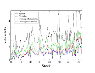
Figure 2: Expected value of spread, first gap, positive and negative spread fluctuations for $71$ stocks in our database. All the quantities are expressed in ticks and the stocks are ordered by size of database. For the definition of these quantities see the text.

The time series describing the dynamics of the spread is characterized by two stylized facts (see, for example, Plerou05 ). First, the unconditional spread distribution has a density function with a fat tail. Some papers suggest that the tail of the spread distribution is well fitted by a power law function Plerou05 ; Mike06 whereas in other studies the spread seems to have an exponential tail Bouchaud06 . The second fact is that spread seems to be described by a long memory process. This implies that the autocorrelation of the spread decays asymptotically as a power law with an exponent smaller than one. Beside these facts there must be a relation between the spread and the variables determining the spread dynamics. These variables are the gap size and the spread variation. The spread is a mean reverting process. Market orders and cancellations at the best can increase the spread whereas limit orders in the spread decrease the spread. An overview of how the spread and related quantities varies across the first 71 stocks in our database is shown in Figure 2. All quantities are sampled every second. We compute the expected spread $E(s(t))$, the expected (symmetrized) first gap $(1/2)E(a_{2}(t)-a(t))+(1/2)E(b(t)-b_{2}(t))$, where $a_{2}(t)$ and $b_{2}(t)$ denote the second ask price level and second bid price level respectively. Here and in the following $E(...)$ indicates an average over time $t$. Moreover, for spread opening fluctuations and spread closing fluctuations, the expectation is taken given there is a fluctuation in either the bid or ask or both. Opening fluctuations consist of the average of $E(a(t+1)-a(t)|a(t+1)>a(t))$ and $E(b(t)-b(t+1)|b(t+1)<b(t))$ with analogous expressions for the closing fluctuations. Finally in the figure the stocks are ordered by size of database. The database size roughly corresponds with activity occurring in each stock during the year 2002, where high activity means a high order submission rate, a high trading rate etc. This therefore suggests that in general the spread, and spread related quantities, decreases with increasing activity. The expected size of spread opening fluctuations is strongly related to the expected size of the first gap when an event removes all the orders at the best price. Similarly the expected size of spread closing fluctuations is strongly related to the expected size of the first gap created by an order submitted into the spread. Fig. 2 shows that spread closing fluctuations are smaller in size than spread opening fluctuations. This means spread closing fluctuations must be more numerous than spread opening fluctuations to maintain a stationary spread. This is therefore a consequence of the slow decay of the spread as will be described below. Since midpoint fluctuations are made up of both opening and closing fluctuations, this figure also suggests that midpoint volatility increases with spread and therefore decreases with activity.

In this paper we are mainly interested in the conditional dynamics of spread. We wish to characterize the dynamics of the spread $s(t)$ conditional to a spread variation. In other words, we wish to answer the question: how does the spread return to a normal value after a spread variation? To this end we compute the quantity

$$G(\tau|\Delta)=E(s(t+\tau)|s(t)-s(t-1)=\Delta)-E(s(t))$$ (1)

Figure 3 shows this quantity for the stock AZN as a function of $\tau$ for different positive and negative values of $\Delta$. The decay of $G(\tau|\Delta)$ as a function of $\tau$ is very slow and for large values of $\tau$ is compatible with a power law decay. In order to obtain better statistics in Figure 4 we plot $G(\tau|\Delta)$ averaged over the $71$ stocks of our sample. As in the individual case the asymptotic decay is compatible with a power law, $G(\tau|\Delta)\sim\tau^{-\delta}$, and the fitted exponent $\delta$ is around $0.4-0.5$. By comparing $G(\tau|\Delta)$ for positive and negative values of $\Delta$ we notice that spread decay conditional to a positive value $\Delta>0$ is very close to the spread decay conditional to the negative value $-\Delta-1$ for time lags longer than few hundreds seconds. We do not have an explanation for this empirical observation. The slow decay of the spread indicates that large changes in the spread are reverted to a normal value with a very slow dynamics. The power law fit suggests that there is not a typical scale for the spread decay. A similar slow decay of the spread was recently observed by Zawadowski et al. in Refs. Kertesz1 ; Kertesz2 . The main difference with this work is that Zawadowski et al. investigated the decay of the spread conditional on a negative change in the midprice rather than in the spread itself. Moreover, the investigated market and database is quite different. Zawadowski et al investigated the NYSE and the NASDAQ by using the Trade and Quote (TAQ) database. They found a slow decay of the spread at NYSE but not at NASDAQ. This does not seem to be consistent with our findings especially when considering the fact that the LSE is probably closer to NASDAQ than to NYSE due to the presence of the specialist at NYSE.

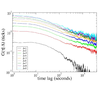
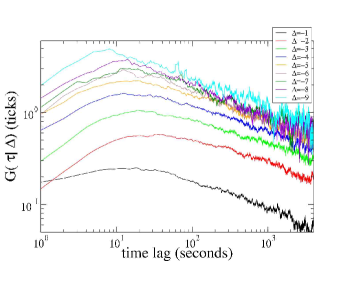
Figure 3: Conditional spread decay $G(\tau|\Delta)$ defined in Eq. 1 for the stock AZN. Top panel shows $G(\tau|\Delta)$ for different positive values of $\Delta$ (in ticks) corresponding to an opening of the spread at time lag $\tau=0$. Bottom panel shows $G(\tau|\Delta)$ for different negative values of $\Delta$ (in ticks) corresponding to a closing of the spread at time lag $\tau=0$.

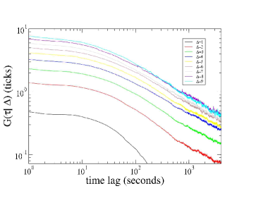
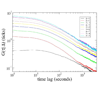
Figure 4: Conditional spread decay $G(\tau|\Delta)$ defined in Eq. 1. The curves are obtained by averaging $G(\tau|\Delta)$ over the 71 stocks of our sample. Top panel shows $G(\tau|\Delta)$ for different positive values of $\Delta$ (in ticks) corresponding to a opening of the spread at time lag $\tau=0$. Bottom panel shows $G(\tau|\Delta)$ for different negative values of $\Delta$ (in ticks) corresponding to a closing of the spread at time lag $\tau=0$.

It is worth noting that the slow spread decay is not a consequence of the long memory property of the spread itself. To show why this is the case, let us consider a generic zero mean stochastic process $x(t)$. The quantity $G(\tau|\Delta)$ is the expectation value $E(x(t+\tau)|x(t)-x(t-1)=y(t)=\Delta)$. In general

$$E(x(t+\tau)y(t))=\int~{}y(t)E(x(t+\tau)|y(t))p(y)~{}dy$$ (2)

thus the $\tau$ dependence of $E(x(t+\tau)y(t))$ is the same as the $\tau$ dependence of $E(x(t+\tau)|y(t))$. For analytical convenience we compute the $\tau$ dependence of $E[x(t+\tau)~{}(x(t)-x(t-1))]$ rather than the conditional expectation of Eq. 1. The quantity $E[x(t+\tau)~{}(x(t)-x(t-1))]$ is equal to $\rho(\tau)-\rho(\tau-1)$, where $\rho(\tau)=E(x(t+\tau)x(t))$ is the autocovariance of $x(t)$. Suppose that $x(t)$ is a long memory process, i.e. that $\rho(\tau)\sim A\tau^{-\beta}$ with $0<\beta<1$. Then our argument shows that

$$E[x(t+\tau)~{}(x(t)-x(t-1))]\sim\frac{A\beta}{\tau^{\beta+1}}.$$ (3)

This result shows that by assuming the spread to be a long memory process with an autocorrelation function decaying as $\tau^{-\beta}$ with $\beta<1$, one should expect that $G(\tau|\Delta)$ decays asymptotically as a power law but with an exponent $1+\beta$ larger than $1$. The fact that the exponent $\delta$ describing the asymptotic decay of $G(\tau|\Delta)$ is significantly smaller than $1$ indicates that the observed slow decay of $G(\tau|\Delta)$ is not a consequence of the long memory property of the spread.

V Determinants of the spread decay

What is the order placement process giving rise to the slow decay of the spread observed in the previous section? The answer to this question is complicated due to the different types of processes that contribute to the spread dynamics. In this section we describe the statistical properties of the events that could contribute to the slow decay of the spread. This approach does not give a full explanation for the decay, but highlights the elements that are relevant for the process.

The dynamics of the spread is determined by the flow of market orders, limit orders falling in the spread and cancellations of the orders at the best bid and ask. The rates of the three different types of orders strongly depend on the spread size. Figure 5 shows the rates (in events per second) of different possible events in the limit order book, specifically trades (market orders), limit orders and cancellations. Limit orders are divided in three subsets according to their limit price. We consider limit orders in the spread, limit orders at an existing best (bid or ask) and limit orders placed inside the book. Similarly cancellations are divided into cancellations of limit orders at the best and cancellations of limit orders inside the book (at the time when they are cancelled). Figure 5 shows that the rate of trading decreases as the spread increases, whereas the rate of limit order submission in the spread dramatically increases with spread size. A similar behavior of the rates of order submission conditional to the spread size has been recently observed by Mike and Farmer Mike06 . This behavior is expected since a large bid-ask spread is a strong disincentive to trade, given that the spread related cost is large. On the other hand, a large spread is an incentive for limit order placement inside the spread in order to have priority of execution at a convenient price. Also the cancellations rate increases with spread. These findings are consistent with a process whereby liquidity providers cancel and replace limit orders in order to slowly close the spread. The increase of the rate of limit order and cancellation at the best and the decrease of market order rate, are consistent with the view of the slow decay of the spread observed in the previous section.

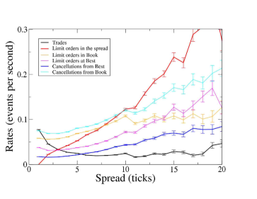
Figure 5: Rates of a series of events in the limit order book conditional to the size of the spread. Limit orders are divided into limit orders in the spread, limit orders at an existing best (bid or ask) and limit orders placed inside the book. Similarly cancellations are divided into cancellations of limit orders at the best and cancellations of limit orders inside the book (at the time when they are cancelled). The data refer to the stock AZN.

The way in which limit orders are placed into the spread when the spread is large is another determinant of the dynamics of spread decay. Limit order placement in the spread follows an interesting scaling relation observed originally by Mike and Farmer Mike06 . In Figure 6 we show the distribution of the distance from the same best of limit orders placed in the spread for different values of the spread. Specifically, given a spread size $s(t)=a(t)-b(t)$ and a limit order with price $p$ between the ask $a(t)$ and the sell $b(t)$, we consider the distribution of $a(t)-p$ for sell limit orders and $p-b(t)$ for buy limit orders. The shape of the curves shown in Figure 6 is consistent with a power law decay with an exponent $\sim 1.8$. Mike and Farmer Mike06 fits the limit order placement with a Student distribution with $1.3$ degrees of freedom. This distribution indicates that when the spread is large, limit orders are not placed simply in a way that immediately reverts the spread back to its typical (small) value. Rather limit orders are sequentially placed close to the existing best price and this leads to a slow decay of the spread.

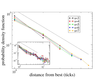
Figure 6: Distribution of the distance between price of limit order in the spread and the best available price (ask for sell limit orders and bid for buy limit orders), for various values of the spread $s$. The inset shows more values of the spread size $s$. The data refer to the stock AZN.

In addition to the investigation of the rate of orders as a function of the size of the spread (Fig. 5) one can also measure the time interval between a spread variation of a given size and the next spread variation (of any size). This waiting time gives the reaction time of the market to an abrupt spread variation. In Figure 7 we show the mean waiting time between a spread variation $\Delta=s(t)-s(t-1)$ and the next spread variation as a function of $\Delta$. The waiting time decreases when the spread variation increases and the functional dependence is approximately logarithmic. In other words the larger the spread variation, the shorter the time one has to wait until a new event changes the spread again. Moreover the waiting time for positive spread variations is much shorter than the waiting time for negative spread variations of the same size (in absolute value). This result is to be expected and shows that the market reacts faster to an increase in the spread rather than to a decrease in the spread. As a last remark on the mean waiting time, we note that there is an oscillation like behavior in the negative spread variation, but we do not have an explanation for this observation.

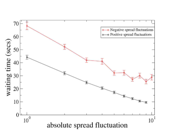
Figure 7: Mean waiting time between a spread variation $\Delta=s(t)-s(t-1)$ and the next spread changing event as a function of $|\Delta|$ for positive (black symbols) and negative (red symbols) spread fluctuations. The figure shows an average of the mean waiting time across the stocks of our sample.

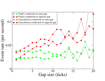
Figure 8: Rate of trades (squares) and cancellations (circles) conditional to the size of the same (green) or opposite (red) gap. The data refer to the stock AZN.

Beside the spread and its fluctuations another important quantity determining liquidity is the gap size. As described above the gap size is the absolute price difference between the best available price (e.g. to buy) and the next best available price. Gap size is important because it has been suggested that immediate price impact is strongly determined by gap size Farmer04 . In any given instant there are two gaps, one on the buy side and one on the sell side of the limit order book. For a buy (sell) market order we define the same side gap size as the gap size on the buy (sell) limit order book side, and opposite side gap size as the gap size on the sell (buy) limit order book side. In Figure 8 we show the trade rate conditional to the same and to the opposite gap size. We see that while the trade rate is almost independent of same side gap size, the rate increases significantly with the opposite side gap size. A possible interpretation of this result is the following. Imagine the market is drifting upward - i.e. the price is increasing. Then most trades are buy initiated and the gap on the sell side is large. Buy limit orders tend to be submitted just inside the spread i.e. beating the best buy by 1 tick, so the gap on the buy side is small.

A similar result is seen for cancellations. Figure 8 also shows the cancellation rate conditional to the size of the same and of the opposite gap. Again it is seen that the cancellation rate weakly depends on the same side gap size, whereas it increases with the size of the opposite gap. When the price is drifting, for example upward, there is a strong limit order flow and cancellation on the buy side of the book. As described above this might be due to the fact that liquidity providers try to gain the best bid by placing buy limit orders in the spread and canceling beaten buy limit orders to get a better position.

VI Permanent impact

In this section we consider the permanent impact of a price fluctuation. The bid or ask can fluctuate in several ways. Firstly a limit order can be submitted into the spread, secondly a cancellation can remove the best, and thirdly a trade can remove the best. The second possibility is rather rare because there are usually several orders at the best owned by different trading agents and they all have to be cancelled independently. On the other hand a single submitted market order can remove all the orders at the best price in one trade. Indeed when a market order arrives in the market, it may trigger a trade which creates a price change. This immediate price change is the immediate impact. The properties of immediate impact as a function of the trading volume and of the market capitalization of the stock have been studied for example in Lillo03 ; Bouchaud03 ; lillocomment . The transaction and the consequent price change generate a cascade of events in reaction. After a sufficiently large period of time the effect of the trade has vanished and the price will be in general different from the price before the trade. The variation of price is the permanent component of the impact of the trade. In this section we are interested in measuring this permanent impact. Since price can fluctuate for different reasons, in the following we distinguish between fluctuation impact and transaction impact. With the first term we refer to the impact on the price conditional to a price fluctuation (caused by any type of event) happening at a previous time. Instead transaction impact is the impact on the price conditional to a fluctuation in the price and to the presence of (at least) a trade at a previous time. Moreover, since there are different prices in the market at a given time (bid, ask, midprice, etc.), we consider the impact on the ask and on the midprice. By considering the ask price fluctuations we can separate the different effects of trades causing positive fluctuations and limit orders falling in the spread causing negative fluctuations

VI.1 Fluctuation Impact

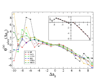
Figure 9: Ask impact $\theta^{(a)}_{after}(\Delta a_{0})$ for 6 highly traded and representative stocks versus $\Delta a_{0}$. The error bars are the standard errors. The inset shows the ask permanent impact averaged across the first 55 stocks of our database, and here the error bars show the stock ensemble average standard errors. Linear regression fits to the points $\Delta a_{0}=1,...,9$ and $\Delta a_{0}=-1,...,-7$ are shown as red lines. For the positive $\Delta a_{0}$ range we find $\theta^{(a)}_{after}(\Delta a_{0})=0.98-0.76\Delta a_{0}$ while for the negative range we obtain $\theta^{(a)}_{after}(\Delta a_{0})=-0.53-0.3\Delta a_{0}$.

As mentioned above fluctuation impact is the impact on the price conditional to a price fluctuation at a previous time. We consider first the permanent impact of ask price fluctuations. Consider the events happening at time $t$. The ask price changes due to these events by a quantity $\Delta a_{0}=a(t)-a(t-1)$, where $a(t)$ is the ask price at the end of second $t$. $\Delta a_{0}$ is the immediate impact. After a sufficiently large time lag $\tau$ the ask price will be $a(t+\tau)$ and the permanent impact is $\Delta a_{perm}(\tau)=a(t+\tau)-a(t-1)$. Thus the permanent impact can be decomposed as

$$\Delta a_{perm}(\tau)=\Delta a_{0}+\Delta a_{after}(\tau)$$ (4)

where $\Delta a_{after}(\tau)=a(t+\tau)-a(t)$ is the price change due to order submission and other events happening after the trade at time $t$ has been completed. $\Delta a_{after}$ is the reaction of the market to the event at time $t$. We measure first the conditional quantity

$$E(\Delta a_{after}(\tau)|\Delta a_{0})=$$ (5)

$$E[a(t+\tau)-a(t)|\Delta a_{0}]-E[a(t+\tau)-a(t)].$$

We subtract the unconditional mean $E[a(t+\tau)-a(t)]$ in order to avoid spurious effects due to the finiteness of the time series. If we let $\tau\to\infty$ then we obtain the permanent impact. Since we cannot take the limit $\tau\to\infty$ in the calculation of the permanent impact, we use as a proxy

$$\theta^{(a)}_{after}(\Delta a_{0})=\frac{1}{T}\sum_{\tau=t_{1}}^{t_{1}+T}E(\Delta a_{after}(\tau)|\Delta a_{0})$$ (6)

where we take $t_{1}=500$ seconds and $T=500$ seconds. In Fig.9 we show $\theta^{(a)}_{after}(\Delta a_{0})$ for some highly traded and representative stocks. We also show the ask impact averaged across the first 55 stocks of our list in the inset presented in the figure.

If the ask price time series is a martingale we expect $\theta^{(a)}_{after}(\Delta a_{0})=0$ independent of $\Delta a_{0}$. That this does not hold is shown in Fig.9. There are large variations across stocks, some showing trend following for small positive $\Delta a_{0}$ and all showing partial reversion for large positive $\Delta a_{0}$. As described above, positive $\Delta a_{0}$ correspond to trade (or cancellation) initiated fluctuations. We note that a one tick positive immediate fluctuation in AZN $\Delta a_{0}=1$, induces on average a further 0.25 tick positive fluctuation in the long time average $\theta^{(a)}_{after}(\Delta a_{0})$. This shows the presence of a trending phase of the ask price in some stocks, which reinforces the direction of the price change. In other stocks, for example BP, a one tick positive ask change induces a negative fluctuation of $\theta^{(a)}_{after}(\Delta a_{0})$ The inset of Fig. 9 shows the average behavior of $\theta^{(a)}_{after}(\Delta a_{0})$ across $55$ stocks. A clear linear behavior of $\theta^{(a)}_{after}(\Delta a_{0})$ as a function of $\Delta a_{0}$ can be seen in different $\Delta a_{0}$ intervals. Also there is a significant asymmetry in $\theta^{(a)}_{after}(\Delta a_{0})$ for positive and negative $\Delta a_{0}$ since their permanent impact behavior is quite different. In particular for the range $\Delta a_{0}=2,...,9$ ticks the points lie on a line of slope approximately $-3/4$, while the $\Delta a_{0}=1$ point is close to zero. In other words, large positive spread fluctuations are partially reverted, while positive one tick spread opening fluctuations are balanced on the long run. The reverting behavior after a large positive ask fluctuation is related to the decay of the large spread opened up by the fluctuation discussed above. This shows that positive ask fluctuations have both a $\Delta a_{0}$ independent part and a part which depends on $\Delta a_{0}$. The total fluctuation composed of the initial fluctuation and of the successive part is $\theta^{(a)}_{perm}(\Delta a_{0})\sim\alpha_{a}+\beta_{a}\Delta a_{0}$, where $\alpha_{a}$ is roughly one tick and $\beta_{a}$ is approximately $1/4$ ticks. Negative ask fluctuations, $\Delta a_{0}=-1$, i.e. orders just beating the ask by one tick, are likely to be followed by further sell orders falling in the spread since they have a trend following permanent impact of approximately $1/2$ tick. This is again the price beating behavior described above. Larger spread closing fluctuations, negative $\Delta a_{0}$, show a negative slope for the range $-2,...-7$. This means that spread closing fluctuations in this range are themselves reverted. This may be because the equilibrium spread is in general not the possible minimum one tick, but maybe several ticks, and smaller spreads than equilibrium may be created by orders falling into the spread which must then revert to equilibrium.

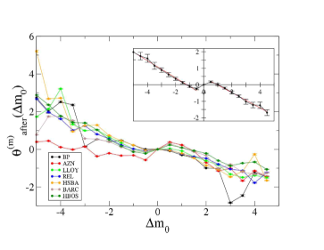
Figure 10: Midprice impact $\theta^{(m)}_{after}(\Delta m_{0})$. The figure shows the result obtained for 6 highly capitalized stocks and the error bars denote standard errors. The inset shows $\theta^{(m)}_{after}(\Delta m_{0})$ averaged across $55$ stocks. In this case the error bars show the stock ensemble average standard errors. Red lines are linear fits.

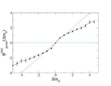
Figure 11: Midprice permanent impact $\theta^{(m)}_{perm}(\Delta m_{0})$ averaged across the first 55 stocks. The error bars show the stock ensemble average standard errors. The red line is the line $y=x$ that would be obtained in case of a permanent impact equal to the immediate impact $\Delta m_{0}$. The green line is the line $y=0$ that would obtained in case of zero permanent impact, i.e. complete reversion.

We now consider the fluctuation impact on the midprice. Midprice permanent impact is defined analogously to the ask price permanent impact as $E(\Delta m_{after}(\tau)|\Delta m_{0})=E[m(t+\tau))-m(t)|\Delta m_{0}]-E[m(t+\tau)-m(t)]$ where $m(t)$ is the midprice at time t and $\Delta m_{0}=m(t)-m(t-1)$ is the mid price one second immediate impact. Again we let $\tau\to\infty$ to obtain the permanent impact

$$\theta^{(m)}_{after}(\Delta m_{0})=\frac{1}{T}\sum_{\tau=t_{1}}^{t_{1}+T}E(\Delta m_{after}(\tau)|\Delta m_{0})$$ (7)

In Fig.10 we show the average of $\theta^{(m)}_{after}(\Delta m_{0})$. As for the ask $\theta^{(m)}_{after}(\Delta m_{0})$ is significantly different from zero independently of $\Delta m_{0}$. Some stocks show quite strong trend following effects for small values of $\Delta m_{0}$ with quite strong reversion effects for large values of $\Delta m_{0}$. For example a half tick positive immediate fluctuation in AZN, $\Delta m_{0}=1/2$, induces on average a further half tick positive fluctuation in the long time average, $\theta^{(m)}_{after}(\Delta m_{0})$ and furthermore a half tick negative immediate fluctuation can induce a further half tick negative permanent change. On the other hand, larger immediate fluctuations are followed by changes of the opposite sign, i.e. partial reversion. There are however quite strong variations across stocks - for example HBOS does not seem to show the strong trend following behavior for small $\Delta m_{0}$ seen in AZN and there is also varying degrees of asymmetry between positive and negative $\Delta m_{0}$ fluctuations. As seen in the inset in Fig.10, the average over the first 55 stocks shows again a clear piecewise linear behavior. When $\Delta m_{0}=1/2$ ($\Delta m_{0}=-1/2$) tick the midprice is on average $0.17$ ($-0.25$) tick. This again shows the presence of a trending phase of the midprice, which reinforces the direction of the price change. For larger price change there is on the contrary a partial reversion of the price. For positive fluctuations the $\Delta m_{0}$ a linear fit gives the relation $\theta^{(m)}_{after}(\Delta m_{0})=0.45-0.46\Delta m_{0}$ while for the negative range we obtain $\theta^{(m)}_{after}(\Delta m_{0})=-0.62-0.52\Delta m_{0}$. The independent part is $0.45$ ticks for positive values of $\Delta m_{0}$ whereas for negative values it is significantly larger, $-0.62$ ticks. In other words negative fluctuations have a larger knock-on effect than positive ones, even for small fluctuations. The total fluctuation including the initial impact, $\theta^{(m)}_{perm}(\Delta m_{0})$ is shown in Figure 11. The permanent impact has a behavior intermediate between the zero impact assumption and the completely permanent impact. From a linear fit of the curve for positive and negative values of $\Delta m_{0}$ we obtain a $\theta^{(m)}_{perm}(\Delta m_{0})=0.45+0.54\Delta m_{0}$ (positive values) and $\theta^{(m)}_{perm}(\Delta m_{0})=-0.62+0.48\Delta m_{0}$ (negative values).

In conclusion the permanent part of the fluctuation impact is roughly linear in the price (ask or mid) that is used as a conditioning variable. The midprice permanent impact is roughly symmetric for positive and negative fluctuations. The ask instead shows a clearly asymmetric profile of the permanent impact. The ask permanent impact $\Delta a_{perm}$ conditional to a given positive ask fluctuation $\Delta a_{0}$ at the initial time is in absolute value smaller than the ask permanent impact conditional to a negative initial ask fluctuation $-\Delta a_{0}$. This asymmetry is a consequence of the different causes for positive and negative ask fluctuations, as well as of the mean reverting and positivity property of spread.

VI.2 Transaction impact

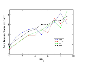
Figure 12: Transaction permanent impact of the ask for three representative stocks and for the averaged pool across the first 55 stocks. Both axes are in tick and we show only the values corresponding to $\Delta a_{0}\geq 0$.

Finally, we consider the transaction impact on the ask, i.e. we measure the permanent impact on the ask conditional to a fluctuation of the ask and to the presence of a transaction at a previous time. Transaction impact is important to assess the permanent effect that a given transaction has on the price. By using the notation of the previous section we measure the quantity

$$E[a(t+\tau)-a(t-1)|\Delta a_{0}~{}AND~{}\exists~{}one~{}buy~{}trade~{}at~{}t]-$$

$$E[a(t+\tau)-a(t-1)].$$ (8)

and, as before, we average this quantity across the range of $\tau$ from $500$ to $1000$ seconds in order to have a proxy of the permanent part. The difference with the previously investigated fluctuation impact is that we now condition also on the presence of at least a buy market order at time $t$. Since buyer initiated trades can produce a zero or a positive fluctuation of the ask, here we consider only the values of the permanent transaction impact of the ask for non negative values of the initial ask fluctuation, $\Delta a_{0}\geq 0$. The permanent transaction impact of the ask is shown in Fig. 12. First of all we note that also when $\Delta a_{0}=0$ there is a $\sim 3/4$ tick permanent ask fluctuation. In other words even when the buyer initiated trade at time $t$ does not change the ask, at time $t+\tau$ the ask is on average $3/4$ ticks higher than the ask at time $t-1$, i.e. just before the trade. This can be due to the fact that liquidity providers raise the ask as a response to a buy market order even if the market order itself does not create a price change. Alternatively it is known that market order signs are significantly correlated in time Bouchaud et al. (2004); Lillo03b . Thus even if a specific buy market order can have vanishing immediate impact, the market order is likely part of a wave of buy market orders that generate a positive permanent impact. From Fig. 12 we note that for $\Delta a_{0}>0$ the permanent transaction impact is roughly proportional to the initial ask fluctuation.

VII Discussion

In this paper, we have shown some empirical facts of limit order book and price dynamics in double auction financial markets, in particular the slow scale-free decay of the spread and the approximately linear permanent market impact function.

The slow spread decay occurring after a sudden opening of the bid-ask spread is certainly affected by the strategic placement of limit orders inside the spread. These strategic limit order submission procedures are performed to attain execution priority at the best ask or bid price after temporary liquidity crises. The scale free decay of the bid-ask spread indicates that the strategies performed might have not a characteristic scale.

The second focus of our paper has been on the permanent price impact induced (i) by any event altering the spread (which we call permanent fluctuation impact) or (ii) by a trade (which we call permanent transaction impact). Our investigations show that the permanent impact is statistically detectable and provides relevant information for the modeling of price formation in high frequency data both on the ask and on the midprice. We observe that the permanent parts of the ask and midprice fluctuation impacts and of the ask and midprice transaction impacts are approximately linear functions of the immediate fluctuation or transaction impact.

This proportionality could be important in the search for the origin of fat tails in price changes. Recently Farmer04 it has been shown that the distribution of non-zero immediate impacts $\Delta m_{0}$ matches the distribution of first gaps very well. This suggests that a major determinant of the origin of large price changes is the presence of large gaps in the limit order book when the market is in a state of lack of liquidity. Clearly the correspondence observed in Farmer04 holds only for individual returns (impact) and it is not a priori obvious that one can extend it to longer time scales. The results in Figs. 11 and 12 give support to the idea that temporary fluctuations of the market liquidity are also responsible for the fat tails of price changes at longer time scales. In fact the distribution of gaps is equal to the distribution of immediate impacts and Figs. 11 and 12 show that permanent impact is a linear function of immediate impact.

- (1) L. Harris, and J. Hasbrouck, Market vs. limit orders: The SuperDOT evidence on order submission strategy, J. Financ. Quant. Anal. 31, 213-231 (1996).
- (2) Y. Hamao, and J. Hasbrouck, Securities trading in the absence of of dealers: Trades and quotes on the Tokyo Stock Exchange, Rev. Financ. Stud., 8, 849-878 (1995).
- (3) B. Biais, P. Hillion, and C. Spatt, An empirical analysis of the limit order book and the order flow in the Paris bourse, J. Financ. 50, 1655-1689 (1995).
- (4) A.W. Lo, A.C. MacKinlay, and J. Zhang, Econometric models of limit order executions, J. Financ. Econom. 65, 31-71 (2002).
- (5) A.D. Hall and N. Hautsch, Order aggressiveness and order book dynamics, Empirical Econom. 30, 973-1005 (2006).
- (6) R.D. Huang, and H.R. Stoll, The components of the Bid-Ask spread: a general approach, Rev. Financ. Stud. 10, 995-1034 (1997).
- (7) B.B. Mandelbrot, The Variation of Certain Speculative Prices, J. Business 36, 394 (1963).
- (8) E.F. Fama, The Behavior of Stock Market Prices, J. Business, 38 34 (1965).
- (9) R.R. Officer, The distribution of stock returns, J. of the American Statistical Assoc. 67, 807-812 (1972).
- (10) V. Akgiray, G.G. Booth, and O. Loistl, Stable Laws Are Inappropriate for Describing German Stock Returns, Allegemeines Statistisches Archiv., 73, 115-121 (1989).
- (11) R.N. Mantegna and H.E. Stanley, Scaling Behavior in the Dynamics of an Economic Index, Nature, 376, 46 (1995).
- (12) F. Longin, The Asymptotic Distribution of Extreme Stock Market Returns, J. of Business 69, 383-408 (1996).
- (13) T. Lux, The stable Paretian hypothesis and the frequency of large returns: an examination of major German stocks, Applied Financial Economics 6, 463-475 (1996).
- (14) P. Gopikrishnan, M. Meyer, L. A. N. Amaral and H. E. Stanley, Inverse cubic law for the distribution of stock price variations, Eur. Phys. J. B 3 139–140 (1998).
- (15) Plerou,V., Gopikrishnan,P., Amaral,L.A.N., Meyer,M., and Stanley, H.E.. Scaling of the distribution of price fluctuations of individual companies Physical Review E 60, 6519-6529 (1999).
- (16) P. K. Clark, A subordinated stochastic process model with finite variance for speculative prices, Econometrica 41 135-256 (1973) .
- (17) X. Gabaix, P. Gopikrishnan, V. Plerou and H. E. Stanley, A theory for power-law distributions in financial market fluctuations, Nature 423 267–270 (2003).
- (18) J. D. Farmer, L. Gillemot, F. Lillo, S. Mike and A. Sen, What really causes large price changes?, Quantitative Finance 4 383–397 (2004).
- (19) V. Plerou, P. Gopikrishnan, and H.E. Stanley. Quantifying fluctuations in market liquidity: Analysis of the bid-ask spread. Phys. Rev. E 71 046131 (2005).
- (20) Mike, S. and Farmer J.D. An empirical behavioral model of price formation preprint at physics/0509194. In press in Journal of Economic Dynamics and Control (2006).
- (21) M. Wyart, J.-P. Bouchaud, J. Kockelkoren, M. Potters, and M. Vettorazzo, Relation between Bid-Ask Spread, Impact and Volatility in Double Auction Markets, preprint at physics/0603084.
- (22) A.G. Zawadowski, J. Kertesz, and G. Andor. Large price changes on small scales. Physica A 344, 221-226 (2004).
- (23) A.G. Zawadowski, G. Andor, and J. Kertesz, Short-term market reaction after extreme price changes of liquid stocks. preprint cond-mat/0406696 (2004)
- (24) Lillo,F. Farmer. J.D. & Mantegna, R.N., Master curve for price-impact Function, Nature 421, 129-130 (2003).
- (25) Potters, M. & Bouchaud, J.-P., More statistical properties of order books and price impact, Physica A 324, 133-140 (2003)
- (26) Farmer, J.D. and Lillo, F., On the origin of power-law tails in price fluctuations, Quantitative Finance 4, C7-C11 (2004).
- Bouchaud et al. (2004) J.-P. Bouchaud, Y. Gefen, M. Potters, and M. Wyart. Fluctuations and response in financial markets: The subtle nature of “random” price changes. Quantitative Finance, 4 176–190, (2004).
- (28) Lillo, F. and Farmer, J.D., The long memory of the efficient market, Studies in Nonlinear Dynamics and Econometrics 8 1 (2004).