Reducing Frustration in Spin Systems: Social Balance as an XOR-SAT problem

Abstract

Reduction of frustration was the driving force in an approach to social balance as it was recently considered by Antal et al. [ T. Antal, P. L. Krapivsky, and S. Redner , Phys. Rev. E 72 , 036121 (2005). ]. We generalize their triad dynamics to $k$-cycle dynamics for arbitrary integer $k$. We derive the phase structure, determine the stationary solutions and calculate the time it takes to reach a frozen state. The main difference in the phase structure as a function of $k$ is related to $k$ being even or odd. As a second generalization we dilute the all-to-all coupling as considered by Antal et al. to a random network with connection probability $w<1$. Interestingly, this model can be mapped onto a $k$-XOR-SAT problem that is studied in connection with optimization problems in computer science. What is the phase of social balance in our original interpretation is the phase of satisfaction of all clauses without frustration in the satisfiability problem of computer science. Nevertheless, although the ideal solution without frustration always exists in the cases we study, it does not mean that it is ever reached, neither in the society nor in the optimization problem, because the local dynamical updating rules may be such that the ideal state is reached in a time that grows exponentially with the system size. We generalize the random local algorithm usually applied for solving the $k$-XOR-SAT problem to a $p$-random local algorithm, including a parameter $p$, that corresponds to the propensity parameter in the social balance problem. The qualitative effect is a bias towards the optimal solution and a reduction of the needed simulation time. We establish the mapping between the $k$-cycle dynamics for social balance on diluted networks and the $k$-XOR-SAT problem solved by a $p$-random local algorithm.

I Introduction

Recently Antal et al. antal proposed a triad dynamics to model the approach of social balance. An essential ingredient in the algorithm is the reduction of frustration in the following sense. To an edge (or link) in the all-to-all topology is assigned a value of $+1$ or $-1$ if it connects two individuals who are friends or enemies respectively. The sign $\pm 1$ of a link we call also its spin. If the product of links along the boundary of a triad is negative, the triad is called frustrated (or imbalanced), otherwise it is called balanced (or unfrustrated). The state of the network is called balanced if all triads are balanced. If the balanced state is achieved by all links being positive the state is called “paradise”. The algorithm depends on a parameter $p\in[0,1]$ called propensity which determines the tendency of the system to reduce frustration via flipping a negative link to a positive one with probability $p$ or via flipping a positive link to a negative with probability $1-p$. For an all-to-all topology Antal et al. predict a transition from imbalanced stationary states for $p<1/2$ to balanced stationary states for $p\geq 1/2$. Here the dynamics is motivated by social applications so that the notion of frustration from physics goes along with frustration in the psychological sense.
Beyond frustration in social systems, within physics, the notion is familiar from spin glasses. It is the degree of frustration in spin glasses which determines the qualitative features of the energy landscape. A high [low] degree of frustration corresponds to many [few] local minima in the energy landscape. In terms of energy landscape it was speculated by Sasai and Wolynes wolynes that is the low degree of frustration in a genetic network which is responsible for the few stable cell states in the high-dimensional space of states.
Calculational tools from spin-glass theory like the replica-method parisi turned out to be quite useful in connection with generic optimization problems (as they occur, for example, in computer science) whenever there is a map between the spin-glass Hamiltonian and a cost function. The goal in finding the ground state-energy of the Hamiltonian translates to the minimization of the costs. A particular class of the optimization problems refers to the satisfiability problems. More specifically one has a system of $B$ Boolean variables and $Q$ logical constraints (clauses) between them. In this case, minimizing the costs means minimizing the number of violated constraints. In case of the existence of a non-violating configuration the problem is said to be satisfiable, it has a zero-ground state energy in the Hamiltonian language. Here it is obvious that computer algorithms designed to find the optimal solution have to reduce the frustration down to a minimal value. So the reduction of frustration is in common to very different dynamical processes.
The algorithms we have to deal with belong to the so-called incomplete algorithms garey ; weigt ; semerjian characterized by some kind of Monte-Carlo dynamics that tries to find the solution via stochastic local moves in configuration space, starting from a random initial configuration. It either finds the solution ”fast” or never (this will be made more precise below). Among the satisfiability problems there are the $k$-SAT ($k$S) problems cook ; mezard ; mezard2 , for which actually no frustration-free solution exists above a certain threshold in the density of clauses imposed on the system. In this case the unsatisfiability is not a feature of the algorithm but intrinsic to the problem. However, there is a special case of $k$S problems, so-called $k$-XOR-SAT ($k$XS) problems weigt ; semerjian ; mezard2 ; cocco which are always solvable by some global algorithm, but poses a challenge for finding the solution by some kind of Monte-Carlo dynamics, very similar to the one used for solving the $k$S problem, where actually no solution may exist. Now it is these $k$XS problems and their solutions that are related to the social balance dynamics.
In particular it can be easily shown mezard ; mezard2 ; cocco that the satisfiability problem $3$S (and also the subclass $3$XS) can first be mapped onto a $3$-spin model that is a spin-glass, and as we shall show below, the $3$-spin glass model can next be mapped onto the triad dynamics of Antal et al. antal . The $k$XS problem is usually studied for diluted connections because the interesting changes in the phase structure of the $k$XS problem appear at certain threshold parameters in the dilution, while the all-to-all case is not of particular interest there.
Dilution of the all-to-all topology is not only needed for the mapping to the $3$XS problem in its usual form. It is also a natural generalization of the triad dynamics considered in antal for social balance. A diluted network is more realistic than an all-to-all topology by two reasons: either two individuals may not know each other at all (this is very likely in case of a large population size) or they neither like or dislike each other, but are indifferent as emphasized in cartwright as an argument for the postulated absence of links. For introducing dilution into the all-to-all network considered by Antal et al. it is quite natural to study random Erdös-Rényi networks erdos for which two nodes are connected by a link with probability $w$. On the other hand, dilution in the $k$XS problem is parameterized by the ratio $\alpha$ of number of clauses over number of variables (variables in the corresponding spin model or number of links in the triad dynamics). We will determine the map between both parameterizations.

In the first part of this paper (section II) we generalize the triad dynamics to $k$-cycle dynamics, driven by the reduction of frustration, with arbitrary integer $k$. In the context of social balance theory, Cartwright and Harary cartwright introduced the notion of balance describing a balanced state with all $k$-cycles being balanced and $k$ not restricted to three. We first study such model on fully connected networks (section III). For given fixed and integer $k\geq 3$ in the updating rules, we draw the differential equations of the time evolution due to the local dynamics (section III.1) and we predict the stationary densities of $k$-cycles, $k$ arbitrary integer, containing $j\leq k$ negative links (section III.2). As long as $k$ is odd (section III.2.1) in the updating dynamics, the results are only quantitatively different from the case of $k=3$ considered in antal . An odd cycle of length three is, however, not an allowed loop in a bipartite graph, for which links may only exist between different type of vertices so that the length of a loop of minimal size in a bipartite graph is four. In addition, a $4$-cycle with four negative links (that is four individuals each of which dislikes two others) is balanced and not frustrated, although it may be called the “hell”, so it does not need to be updated in order to reduce its frustration. (To call the hell with four negative links balanced is not specific for the notion of frustration in physics; also in social balance theory it is the product over links in the loop which counts and decides about balance or frustration roberts .) This difference is essential as compared to the triad dynamics, in which a triad of three unfriendly links is always updated. It has important implications on the phase structure as we will show. For even values of $k$ and larger than four, again there are only quantitative differences in the phase structure as compared to $k=4$ (section III.2.2).
As in antal , for odd values of $k$, we shall distinguish between stationary states in the infinite volume limit that can be either balanced (for $p\geq 1/2$) or frustrated (for $p<1/2$) since it is not possible to reach the paradise in a finite time. They are predicted as solutions of mean field equations. In numerical simulations, fluctuations about their stationary values do not die out in the phase for $p<1/2$ so that some frustration remains, while for $p\geq 1/2$ frozen states are always reached in the form of the paradise although other balanced states with a finite amount of negative links are in principle available, but are quite unlikely to be realized during the finite simulation time. They are exponentially suppressed due to their small weight in configuration space. We calculate the time it takes to reach a frozen state at and above the phase transition (section III.3.1). For even values of $k$ we have only two types of stationary frozen states, “paradise” and “hell” with all links being positive and negative, respectively. In this case the time to reach the frozen states at the transition can be calculated in two ways. The first possibility applies for both even and odd values of $k$ and is based on calculating the time it takes until a fluctuation is of the same order in size as the average density of unfriendly links. The second one, applicable to the case of even values of $k$, can be obtained by mapping the social system to a Markov process known as the Wright-Fisher model for diploid organisms wright , for which the decay time to one of the final configurations (all “positive” or all “negative” genes) increases quadratically in the size $N$ of the system (section III.3.2).
In the second part we generalize the $k$-cycle dynamics to diluted systems (section IV). The dilution, originally given in terms of the probability for connecting two links in a random Erdös-Rényi network erdos , is then parameterized in terms of the dilution parameter $\alpha$, and the results for stationary and frozen states and the time needed to reach them will be given as a function of $\alpha$ (section IV.1). The original triad dynamics of Antal et al. with propensity parameter $p$ on a diluted network contains, as special case, the usual Random-Walk SAT (RWS) algorithm for finding the solution of the $3$XS problem corresponding to the choice of $p=1/3$ in the triad dynamics. Therefore it is natural to generalize the RWS algorithm for generic $p\in[0,1]$ and to study the modifications in the performance of the algorithm as a function of $p$ (section IV.2). For the $k$S problem, and similarly for the $k$XS problem, there are three thresholds in $\alpha$, $\alpha_{d}$, $\alpha_{s}$, and $\alpha_{c}$ with $\alpha_{d}<\alpha_{s}<\alpha_{c}$. Roughly speaking, the threshold $\alpha_{d}$ corresponds to a dynamical transition between a phase in which the RWS algorithm finds a solution in a time linearly increasing with the size of the system for $\alpha<\alpha_{d}$, and exponentially increasing with the system size for $\alpha>\alpha_{d}$. The value $\alpha_{s}$ characterizes a transition in the structure of the solution space, from one cluster of exponentially many solutions ($\alpha<\alpha_{s}$) to exponentially many clusters of solutions ($\alpha>\alpha_{s}$). Finally, $\alpha_{c}$ refers to the transition between satisfiable and unsatisfiable $k$S problems, this means that for these models not all constraints can be satisfied simultaneously in the UNSAT-phase for $\alpha>\alpha_{c}$ so that a finite amount of frustration remains. Above this last threshold lies a value of $\alpha,\;\alpha=\alpha_{m}$, such that for $\alpha>\alpha_{m}$ the mean field approximation is justified that was used for the maximum value of $\alpha$ in the all-to-all topology of the triad dynamics of antal . We shall study the influence of the parameter $p$ on the value of $\alpha_{d}$ (section IV.2.1) and on the Hamming distance for $\alpha$ smaller $\alpha_{s}$ or larger $\alpha_{s}$ (section IV.2.2). Moreover we will show how the choice of $p$ changes the possibility to find a solution for the $k$XS problem (section IV.2.3) and we will determine the validity range of the mean-field approximation (section IV.2.4). As it turns out, the parameter $p$ introduces some bias in the RWS, accelerating the convergence to “paradise” and reducing the explored part of configuration space. On the other hand, an inappropriate choice of $p$ or too much dilution may prevent an approach to paradise. Fluctuations in the wrong direction, increasing the amount of frustration, go along with improved convergence to the balanced state.

II The Model for Social Balance

We represent individuals as vertices (or nodes) of a graph and a relationship between two individuals as a link (or edge) that connects the corresponding vertices. Moreover we assign to a link $(i,j)$ between two nodes $i$ and $j$ a binary spin variable $s_{i,j}=\pm 1$, with $s_{i,j}=1$ if the individuals $i$ and $j$ are friends , and $s_{i,j}=-1$ if $i$ and $j$ are enemies. We consider the standard notion of social balance extended to cycles of order $k$ cartwright ; heider . In particular a cycle of order $k$ (or a $k$-cycle) is defined as a closed path between $k$ distinct nodes $i_{1}$, $i_{2}$, …, $i_{k}$ of the network, where the path is performed along the links of the network $(i_{1},i_{2})$ , $(i_{2},i_{3})$ , …, $(i_{k-1},i_{k})$, $(i_{k},i_{1})$. Given a value of $k$ we have $k+1$ different types $T_{0}$, $T_{1}$, …, $T_{j}$, …, $T_{k}$ of cycles of order $k$ containing $0$, $1$, …, $j$, …, $k$ negative links, respectively. A cycle of order $k$ in the network is considered as balanced if the product of the signs of links along the cycle equals $1$, otherwise the cycle is considered as imbalanced or frustrated. Accordingly, the network is considered as balanced if each $k$-cycle of the network is balanced.
We consider our social network as a dynamical system. We perform a local unconstrained dynamics obtained by a natural generalization of the local triads dynamics, recently proposed by Antal et al. antal . We first fix a value of $k$. Next, at each update we choose at random a $k$-cycle $T_{j}$. If this $k$-cycle $T_{j}$ is balanced ($j$ is even) nothing happens. If $T_{j}$ is imbalanced ($j$ is odd) we change one of its link as follows: if $j<k$, then $T_{j}\to\;T_{j-1}$ occurs with probability $p$, while $T_{j}\to\;T_{j+1}$ occurs with probability $1-p$ ; if $j=k$, then $T_{j}\to\;T_{j-1}$ happens with probability $1$. During one update, the positive [negative] link which we flip to take a negative [positive] sign is chosen at random between all the possible positive [negative] links belonging to the $k$-cycle $T_{j}$. One unit of time is defined as a number of updates equal to $L$, where $L$ total number of links of the network. In Figure 1 we show a simple scheme that illustrates the dynamical rules in the case $k=4$ (A) and $k=5$ (B). It is evident from the figure that for even values of $k$ the system remains the same if we simultaneously flip all the spins $s_{i,j}\to-s_{i,j}$ $\forall\;(i,j)$ and make the transformation $p\to 1-p$. The same is not true for odd values of $k$. The reason is that a $k$-cycle with only “unfriendly” links is balanced for even values of $k$, while it is imbalanced for odd values of $k$. The presence or absence of this symmetry property for even values of $k$ or odd, respectively, is responsible for very different features in the phase structure. This will be studied in detail in the following sections.

Figure 1: Dynamical rules in case of $k=4$ (A) and $k=5$ (B). The cycles containing an odd number of “unfriendly” links are considered as imbalanced and evolve into balanced ones. Full and dashed lines represent “friendly” and “unfriendly” links respectively.

III Complete graphs

We first consider the case of fully connected networks. Later we extend the main results to the case of diluted networks in section IV. In a complete graph every individual has a relationship with everyone else. Let $N$ be the number of nodes of this complete graph. The total number of links of the network is then given by $L={N\choose 2}$, while the total number of $k$-cycles is given by $M={N\choose k}$. ${x\choose y}$ is the standard notation of the binomial coefficient. It counts the total number of different ways of choosing $y$ elements out of $x$ elements in total, while it is $0\leq y\leq x$ , with $x,y\in\mathbb{N}$. Moreover we define $M_{j}$ as the number of $k$-cycles containing $j$ negative links, and $m_{j}=\;M_{j}/\;M$ the respective density of $k$-cycles of type $T_{j}$. The total number of positive links $L^{+}$ is then related to the number of $k$-cycles by the relation

$$L^{+}=\frac{\sum_{i=0}^{k}\left(k-i\right)\;M_{i}}{\left(N-2\right)!\;/\;\left(N-k\right)!}\;\;\;.$$ (1)

A similar relation holds for the total number of negative links $L^{-}$

$$L^{-}=\frac{\sum_{i=0}^{k}i\;M_{i}}{\left(N-2\right)!\;/\;\left(N-k\right)!}\;\;\;.$$ (2)

In particular, in Eq.s (1) and (2) the numerators give us the total number of positive and negative links in all the $k$-cycles, respectively, while the same denominator comes out from the fact that one link belongs to $(N-2)(N-3)\cdots(N-k+1)=\left(N-2\right)!/\left(N-k\right)!$ different $k$-cycles. Furthermore the density of positive links is $\rho=L^{+}/L=1-\sum_{i=0}^{k}\;i\;m_{i}$, while the density of negative links is $1-\rho$.

III.1 Evolution Equations

In view of deriving the mean field equations for the unconstrained dynamics, introduced in the former section II, we need to define the quantity $M^{+}_{j}$ as the average number of $k$-cycles of type $T_{j}$ which are attached to a positive link. This number is given by

$$M^{+}_{j}=\frac{\left(k-j\right)\;\;M_{j}}{L^{+}}\;\;\;,$$

while similarly

$$M^{-}_{j}=\frac{j\;\;M_{j}}{L^{-}}$$

counts the average number of $k$-cycles of type $T_{j}$ attached to a negative link. In term of densities we can easily write

$$m^{+}_{j}=\frac{\left(k-j\right)\;\;m_{j}}{\sum_{i=0}^{k}\;\left(k-i\right)\;m_{i}}$$ (3)

and

$$m^{-}_{j}=\frac{j\;\;m_{j}}{\sum_{i=0}^{k}\;i\;m_{i}}\;\;\;.$$ (4)

Now let $\pi^{+}$ be the probability that a link flips its sign from positive to negative in one update event and $\pi^{-}$ the probability that a negative link changes its sign to $+1$ in one update event. We can write such probabilities as

$$\pi^{+}=\left(1-p\right)\;\sum_{i=1}^{(k-1)/2}\;m_{2i-1}$$ (5)

and

$$\pi^{-}=p\;\sum_{i=1}^{(k-1)/2}\;m_{2i-1}\;+\;\;m_{k}\;\;\;,$$ (6)

valid for the case odd values of $k$. For even values of $k$, these probabilities read

$$\pi^{+}=\left(1-p\right)\;\sum_{i=1}^{k/2}\;m_{2i-1}$$ (7)

and

$$\pi^{-}=p\;\sum_{i=1}^{k/2}\;m_{2i-1}\;\;\;.$$ (8)

Since each update changes $\left(N-2\right)!/\left(N-k\right)!$ $k$-cycles, and also the number of updates in one time step is equal to $L$ update events, the rate equations in the mean field approximation can be written as

$$\left\{\begin{array}[]{l}\frac{d}{dt}\;m_{0}\;=\;\pi^{-}\;m^{-}_{1}\;-\;\pi^{+}\;m^{+}_{0}\\ \\ \begin{array}[]{ll}\frac{d}{dt}\;m_{1}\;=&\pi^{+}\;m^{+}_{0}\;+\;\pi^{-}\;m^{-}_{2}\;+\\ &-\;\pi^{-}\;m^{-}_{1}\;-\;\pi^{+}\;m^{+}_{1}\end{array}\\ \vdots\\ \begin{array}[]{ll}\frac{d}{dt}\;m_{j}\;=&\pi^{+}\;m^{+}_{j-1}\;+\;\pi^{-}\;m^{-}_{j+1}\;+\\ &-\;\pi^{-}\;m^{-}_{j}\;-\;\pi^{+}\;m^{+}_{j}\end{array}\\ \vdots\\ \begin{array}[]{ll}\frac{d}{dt}\;m_{k-1}\;=&\pi^{+}\;m^{+}_{k-2}\;+\;\pi^{-}\;m^{-}_{k}\;+\\ &-\;\pi^{-}\;m^{-}_{k-1}\;-\;\pi^{+}\;m^{+}_{k-1}\end{array}\\ \\ \frac{d}{dt}\;m_{k}\;=\;\pi^{-}\;m^{-}_{k-1}\;-\;\pi^{-}\;m^{-}_{k}\end{array}\right.\;\;\;.$$ (9)

We remark that the only difference between the cases of odd values of $k$ and even values of $k$ comes from Eq.s (5) and (6), and Eq.s (7) and (8), respectively. This difference is the main reason why the two cases odd values of $k$ and even values of $k$ lead to two completely different behavior and why we treat them separately in the following section III.2.

III.2 Stationary states

Next let us derive the stationary states from the rate equations (9) that give a proper description of the unconstrained dynamics of $k$-cycles in a complete graph. Imposing the stationary condition $\frac{d}{dt}\;m_{j}=0$ , $\forall\;0\leq j\leq k$, we easily obtain

$$m^{+}_{j-1}\;=\;m^{-}_{j}\;\;\;,\;\forall\;1\leq j\leq k\;\;\;.$$ (10)

Then, forming products of the former quantities appearing in Eq.(10), we have

$$m^{+}_{j-1}\;m^{-}_{j+1}\;=\;m^{+}_{j}\;m^{-}_{j}\;\;\;,\;\forall\;1\leq j\leq k\;\;$$

and, using the definitions of Eq.s (3) and (4), we finally obtain

$$\left(k-j+1\right)\left(j+1\right)\;m_{j-1}\;m_{j+1}\;\;=\;\;\left(k-j\right)j\left(\;m_{j}\;\right)^{2}\;\;\;,$$ (11)

valid $\forall\;1\leq j\leq k$. Moreover the normalization condition $\sum_{i}\;m_{i}\;=\;1$ should be satisfied. Furthermore, in the case of stationary, the density of friendships should be fixed, so that we should impose that $\pi^{+}\;=\;\pi^{-}$.

III.2.1 The case of odd values of $k$

In the case of odd values of $k$, the condition for having a fixed density of friendships reads

$$m_{k}\;=\;\left(1-2p\right)\;\sum_{i=1}^{(k-1)/2}\;m_{2i-1}\;\;\;,$$ (12)

where we used Eq.s (5) and (6). In principle the $k$ equations of (11) plus the normalization condition and the fixed friendship relation (12) determine the stationary solution. For $k=3$ Antal et al. antal found

$$m_{j}\;=\;{3\choose j}\;\rho_{\infty}^{3-j}\;\left(1-\rho_{\infty}\right)^{j}\;\;,\;\forall\;0\leq j\leq 3\;\;\;,$$ (13)

where

$$\rho_{\infty}\;=\;\left\{\begin{array}[]{ll}1/\left[\sqrt{3\left(1-2p\right)}+1\right]&\textrm{ , if }p\leq 1/2\\ 1&\textrm{ , if }p\geq 1/2\end{array}\right.$$ (14)

is the stationary density of friendly links. In the same manner also the case $k=5$ can be solved exactly with the solution

$$m_{j}\;=\;{5\choose j}\;\rho_{\infty}^{5-j}\;\left(1-\rho_{\infty}\right)^{j}\;\;,\;\forall\;0\leq j\leq 5\;\;\;,$$ (15)

where

$$\rho_{\infty}\;=\;\left[\sqrt{5\left(1-2p\right)\left(1+\sqrt{1+\frac{1}{5(1-2p)}}\right)}+1\right]^{-1}$$ (16)

for $p\leq 1/2$, while $\rho_{\infty}=1$ for $p\geq 1/2$.
In Figure 2 we plot the densities $m_{j}$ given by Eq.(15) and the stationary density of friendly links $\rho_{\infty}$ given by Eq.(16) as function of $p$. Moreover we verified the validity of the solution performing several numerical simulations on a complete graph with $N=64$ nodes (full dots). We compute numerically the average density of positive links after $10^{3}$ time steps, where the average is done over $10^{2}$ different realizations of the system. At the beginning of each realization we select at random the values of the signs of the links, where each of them has the same probability to be positive or negative, so that $\rho_{0}=0.5$. The numerical results perfectly reproduce our analytical predictions.

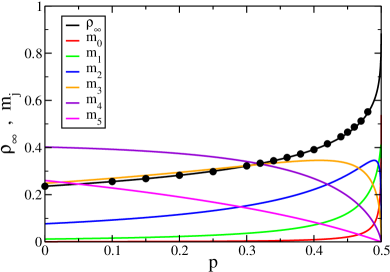
Figure 2: (Color online) Exact stationary densities $m_{j}$ for the cycles of order $k=5$ from Eq.(15) and stationary density of friendly links $\rho_{\infty}$ from Eq.(16), both as a function of the dynamical parameter $p$. Numerical results are also reported for a system with $N=64$ vertices. Each value (full dot) is obtained by averaging the density of friendly links reached after $10^{3}$ time steps over $10^{2}$ different realizations with random initial conditions ($\rho_{0}=0.5$).

As one can easily see, both solutions (13) and (15) are just binomial distributions. This means that the densities of a cycle of order $k=3$ or a cycle of order $k=5$ with $j$ negative links are simply given by the probability of finding these densities on a complete graph in which each link is set equal to $1$ with probability $\rho_{\infty}$ or equal to $-1$ with probability $1-\rho_{\infty}$. (As already noticed in antal , this result may come a bit as a surprise, because the $3$-cycle or here the $5$-cycle dynamics seems to be biased towards the reduction of frustration, on the other hand it is a bias for individual triads without any constraint of the type that the frustration of the whole ”society” should get reduced.)
For odd values of $k>5$, a stationary solution always exists. This solution becomes harder to find as $k$ increases, because the maximal order of the polynomials involved increases with $k$ (for $k=3$ we have polynomials of first order, for $k=5$ polynomials of second order, for $k=7$ of third and so on). So it becomes impossible to find the solution analytically as the maximal order of solvable equations is reached. Nevertheless we can give an approximate solution using a self-consistent approach as we shall outline in the following. We suppose that the general solution for the stationary densities is of the form

$$m_{j}\;=\;{k\choose j}\;\rho_{\infty}^{k-j}\;\left(1-\rho_{\infty}\right)^{j}\;\;,\;\forall\;0\leq j\leq k\;\;\;,$$ (17)

Eq.(17) is an appropriate ansatz as we can directly see from the definition of the density of friendly links $\rho_{\infty}=1-\sum_{i=0}^{k}i\;m_{i}=1-(1-\rho_{\infty})$, where the last term comes out as mean value of the binomial distribution. ( Actually such self-consistency condition is satisfied by any distribution of the $m_{j}$s with mean value equal to $1-\rho_{\infty}$. ) Moreover the ansatz for the stationary solution in the form of Eq.(17) has the following features: first it is valid for the special cases $k=3$ and $k=5$, and second, it is numerically supported. In Figure 3 we show some results obtained by numerical simulations. We plot the densities $m_{j}$ for different values of $k$ [ $k=7$ (A) , $k=9$ (B), $k=11$ (C) and $k=21$ (D) ] and different values of $p$ [ $p=0$ (black circles) , $p=0.3$ (red squares) , $p=0.44$ (green diamonds) and $p=0.49$ (blue crosses) ]. We performed $50$ different realizations of a system of $N=64$ vertices, where the densities are extrapolated from $10^{6}$ samples ($k$-cycles) at each realization and after $5\cdot 10^{2}$ time steps of the simulations (so that we have reached the stationary state). The initial values of the signs are chosen to be friendly or unfriendly with the same probability ($\rho_{0}=0.5$). The full lines are given by Eq.(17) for which the right value of $\rho_{\infty}$ is given by the average stationary density of friendly links and the average is performed over all simulations. Furthermore, we numerically check whether Eq.(17) holds, with the same $\rho_{\infty}$ if we measure the densities of cycles also of order $k^{\prime}\neq k$ and moreover, whether it holds during the time while using the time dependent density of friendly links $\rho(t)$ instead of the stationary one $\rho_{\infty}$. Since all these checks are positive, we may say that if at some time the distribution of friendly links (and consequently of unfriendly links) is uncorrelated, it will stay so forever.

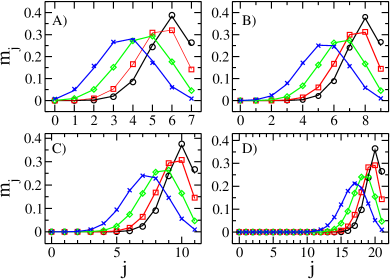
Figure 3: (Color online) Stationary densities $m_{j}$ for the $k$-cycles with $j$ negative links and different values of $k$ [ $k=7$ (A) , $k=9$ (B), $k=11$ (C) and $k=21$ (D) ], and for different values of $p$ [ $p=0$ (black circles) , $p=0.3$ (red squares) , $p=0.44$ (green diamonds) and $p=0.49$ (blue crosses) ]. The numerical results (symbols) represent the histograms extrapolated from $10^{6}$ samples and over $50$ different realizations of the network. In particular the initial values of the spins are equally likely at each realization (so that $\rho_{0}=0.5$), the distributions are sampled after $5\cdot 10^{2}$ time steps and the system size is always $N=64$. The prediction of Eq.(17) is plotted as a full line and the value of $\rho_{\infty}$ used is taken from the simulations as the average value of the stationary density of positive links.

Let us assume that the ansatz (17) is valid, we then evaluate the unknown value of $\rho_{\infty}$ self-consistently by imposing the condition that the density of friendly links is fixed at the stationary state

$$\pi^{+}\;=\;\pi^{-}\;\;\;\Leftrightarrow\;\;\left(1-2p\right)\sum_{i=1}^{(k-1)/2}\;m_{2i-1}\;=\;m_{k}\;\;\;.$$

In particular we can write

$$\sum_{i=1}^{(k-1)/2}\;m_{2i-1}\;+\;m_{k}\;=\;\sum_{i=1}^{(k+1)/2}\;m_{2i-1}\;=\xi\;,$$ (18)

and so

$$m_{k}\;=\;\left(1-2p\right)\left(\xi-\;m_{k}\right)\;$$

from which

$$\rho_{\infty}\;=\;1-\left[\frac{\xi\left(1-2p\right)}{2\left(1-p\right)}\right]^{1/k}\;\;\;,$$ (19)

for $p\leq 1/2$, while $\rho_{\infty}=1$ for $p\geq 1/2$. In particular we notice that Eq.(19) goes to zero as $k\to\infty$ for $p<1/2$, because $0\leq\xi\leq 1$.. This means that in the limit of large $k$ the stationary density of friendly links takes the typical shape of a step function centered at $p=1/2$, with $\rho_{\infty}=0$ for $p<1/2$ and $\rho_{\infty}=1$ for $p>1/2$. This is exactly the result we find for the case even values of $k$ (see the next section III.2.2), and it is easily explained since in the limit of large $k$ the distinction between the cases odd values of $k$ and $k$ even should become irrelevant.
Furthermore it should be noticed that $\xi$ defined in Eq.(18) is nothing more than a sum of all odd terms of a binomial distribution. For large values of $k$ we should expect that the sum of the odd terms is equal to the sum of the even terms of the distribution, so that

$$\xi\;=\;\sum_{i=1}^{(k+1)/2}\;m_{2j-1}\;\simeq\frac{1}{2}\;\simeq\;\sum_{i=0}^{(k-1)/2}\;m_{2j}\;\;\;,$$

because of the normalization. In Figure 4 we plot the quantity $(1-\rho_{\infty})^{k}$ obtained by numerical simulations for different values of $k$ [ $k=3$ (black circles) , $k=5$ (red squares) , $k=7$ (blue diamonds) , $k=9$ (violet triangles), $k=11$ (orange crosses) ] as a function of $p$. Each point represents the average value of the density of positive links (after $10^{3}$ time steps) over $10^{2}$ different realizations. The system size in our simulations is $N=64$, while, at the beginning of each realization, the links have the same probability to have positive or negative spin ($\rho_{0}=0.5$). From Eq.(19) we expect that the numerical results collapse on the same curve $\xi(1-2p)/(2-2p)$, depending on the parameter $\xi$. Imposing $\xi=1/2$ [dashed line] we obtain an excellent fit for all values of $p$. Only for small values of $p$ the fit is less good than for intermediate and large values of $p$, which is explained by the plot in the inset of Figure 4. There Eq.(18) is shown as function of $p$ for $k=3$ (black dotted line) and for $k=5$ (red full line). The values of $m_{j}$ are taken directly from the binomial distribution of Eq.(17) with values of $\rho_{\infty}$ known exactly from Eq.s (14) and (16) for $k=3$ and $k=5$, respectively. We can see how well the approximation $\xi=1/2$ works already for $k=3$ and how it improves for $k=5$, with the only exception for small values of $p$ where $\xi>1/2$. Furthermore we see that $\xi<1/2$ for $p\simeq 1/2$, but in this range the dependence on $\xi$ of Eq.(19) becomes weaker since the factor $\xi(1-2p)$ tends to zero anyway.

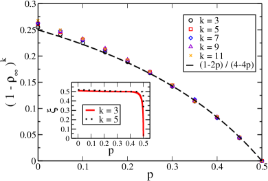
Figure 4: (Color online) Numerical results (symbols) and approximate solution (dashed line) for the function $\left(1-\rho_{\infty}\right)^{k}$, depending on the stationary density of positive links $\rho_{\infty}$ and the parameter $k$ [ $k=3$ (black circles) , $k=5$ (red squares) , $k=7$ (blue diamonds) , $k=9$ (violet triangles) , $k=11$ (orange crosses) ], as a function of the dynamical parameter $p$. The theoretical result, plotted here as a dashed line, is given by Eq.(19) for $\xi=1/2$. This prediction is in good agreement with the numerical results obtained by averaging the density of friendly links after $10^{3}$ time steps over $10^{2}$ different realizations. The system size is $N=64$. Each simulation starts with random initial conditions ($\rho_{0}=0.5$). Moreover, as we can see from the inset, the value of $\xi$ calculated for $k=3$ (red full line) and for $k=5$ (black dotted line) is very close to $1/2$ for an extended range of $p$.

III.2.2 The case of even values of $k$

The stability of a $k$-cycle with all negative links in the case of even $k$ (see Figure 1) has deep implications on the global behavior of the model. Actually the elementary dynamics is now symmetric. Only the value of $p$ gives a preferential direction (towards a completely friendly or unfriendly cycle) to the basic processes. With odd $k$, for $p<1/2$ the tendency of the dynamics to reach the state with a minor number of positive links in the elementary processes (involving no totally unfriendly cycles) is overbalanced by the process $T_{k}\rightarrow T_{k-1}$ which happens with probability one, so that in the thermodynamical limit the system ends up in an active steady state with a finite average density of negative links due to the competition between the basic processes. Instead, for even $k$, nothing prevents the system from reaching the “hell”, that is a state of only negative links, because here a completely negative cycle is stable. Only for $p=1/2$ we expect to find a non-frozen fluctuating final state, since in this case the elementary dynamical processes are fully symmetric. Imposing the stationary conditions on the system we do not get detailed information about the final state. As we can see from Eq.s (7) and (8), for $p\neq 1/2$ the only possibility to have $\pi^{+}=\pi^{-}$ is the trivial solution for which both probabilities are equal to zero, so that the system must reach a frozen configuration, while for $p=1/2$, $\pi^{+}$ and $\pi^{-}$ are always equal, in this case we expect the system to reach immediately an active steady state. In order to describe more precisely the final configuration of this active steady state, it is instructive to consider the mean-field equation for the density of positive links. For generic even value of $k$, it is easy to see that the number of positive links increases in updates of type $T_{2j-1}\rightarrow T_{2(j-1)}$ with probability $p$, whereas it decreases in updates of type $T_{2j-1}\rightarrow T_{2j}$ with probability $1-p$, so that the mean field equation that governs the behavior of the density of friendly links is given by

$$\frac{d\rho}{dt}=(2p-1)\rho(1-\rho)\cdot\sum_{i=1}^{k/2}{k\choose 2i-1}\cdot\rho^{k-2i}(1-\rho)^{2(i-1)}\;\;\;.$$ (20)

For $p\neq 1/2$ we have only two stationary states, $\rho_{\infty}=0$ and $\rho_{\infty}=1$ (the other roots of the steady state equation are complex). It is easily understood that for $p<1/2$ the stable configuration is $\rho_{\infty}=0$, while for $p>1/2$ it is $\rho_{\infty}=1$. In contrast, for $p=1/2$ we have $\rho(t)=$const at any time, so that $\rho_{\infty}=\rho(t=0)=\rho_{0}$. These results are confirmed by numerical simulations. Moreover, the convergence to the thermodynamical limit is quite fast, as it can be seen in Figure 5, where we plot the density of friendly links $\rho_{\infty}$ as a function of $p$ for the system sizes $N$ [ $N=8$ (dotted line), $N=16$ (dashed line) and $N=32$ (full line) ] and for $k=4$. Each curve is obtained from averages over $10^{3}$ different realizations of the dynamical system. In all simulations the links get initially assigned the values $\pm 1$ with equal probability, so that $\rho_{0}=0.5$.

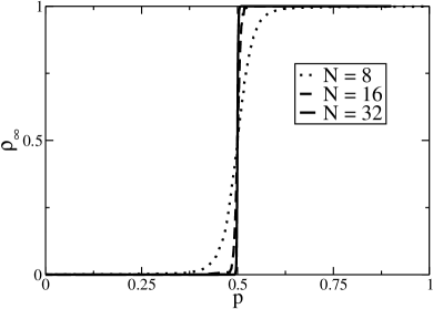
Figure 5: Behavior of the stationary density of friendly links $\rho_{\infty}$ as a function of $p$ for three (small) values of $N$ [ $N=8$ (dotted line), $16$ (dashed line) and $32$ (full line) ] and for $k=4$. The values of the initial configuration are randomly chosen to be $\pm 1$ with density of friendly links $\rho_{0}=0.5$. The curves are obtained from averages over $10^{3}$ different realizations.

III.3 Frozen configurations

When all $k$-cycles of the network are balanced we say that the network itself is balanced. In particular, in the case of our unconstrained dynamics we can say that if the network is balanced it has reached a frozen configuration. The configuration is frozen in the sense that no dynamics is left since the system cannot escape a balanced configuration. Furthermore it was proven cartwright that if a graph (not only a complete graph) is balanced it is balanced independently of the choice of $k$ and that the only possible balanced configurations are given by bipartitions of the network in two subgroups (or “cliques”), where all the individuals belonging to the same subgroup are friends while every couple of individuals belonging to different subgroups are enemies (this result is also known as Structure Theorem roberts ). In the case of even values of $k$ the latter result is still valid if all the individuals of one subgroup are enemies, while two individuals belonging to different subgroups are friends. It should be noticed that one of the two cliques may be empty and therefore the configuration of the paradise (where all the individuals are friends) is also included in this result, as well as, for the case even values of $k$, the hell with all individuals being enemies . In the following we will combine our former results about the stationary states (section III.2) with the notion of frozen configurations in order to predict the probability of finding a particular balanced configuration and the time needed for freezing our unconstrained dynamical process. For clarity we analyze the cases of odd values of $k$ and even values of $k$ separately, again.

III.3.1 Freezing time for odd values of $k$

Let $0\leq N_{1}\leq N$ be the size of one of the two cliques. Therefore the other clique will be of size $N-N_{1}$. In such a frozen configuration the total number of positive and negative links are related to $N_{1}$ and $N$ by

$$L^{+}=\frac{N_{1}\left(N_{1}-1\right)}{2}+\frac{\left(N-N_{1}\right)\left(N-N_{1}-1\right)}{2}$$ (21)

and

$$L^{-}=N_{1}\left(N-N_{1}\right)$$ (22)

respectively. As we have seen in the former section III.2.1, for odd values of $k$ and $p<1/2$, all the $k$-cycles are uncorrelated during the unconstrained dynamical evolution, if we start from an initially uncorrelated configuration. In such cases, we can consider our system as a purely random process in which the values of the spins are chosen at random with a certain probability. In particular, the probability of a link to be positive is given by $\rho$ , the density of positive links ( $1-\rho$ is the probability for a link to be negative). The probability of reaching a frozen configuration, characterized by two cliques of $N_{1}$ nodes and $N-N_{1}$ nodes, is then given by

$$P(\rho,N_{1})={N\choose N_{1}}\rho^{\frac{N(N-1)}{2}-N_{1}(N-N_{1})}\left(1-\rho\right)^{N_{1}(N-N_{1})}\;\;\;.$$ (23)

The binomial coefficient ${N\choose N_{1}}$ in Eq.(23) counts the total number of possible bi-partitions into cliques with $N_{1}$ and $N-N_{1}$ nodes ( i.e. the total number of different ways for choosing $N_{1}$ nodes out of $N$), and each of these bi-partitions is considered as equally likely because of the randomness of the process. We should also remark that in Eq.(23) we omit the time dependence of $\rho$, while the density of positive links $\rho$ follows the following master equation

$$\frac{d\rho}{dt}=(1-\rho)^{k}+(2p-1)\sum_{i=1}^{(k-1)/2}{k\choose 2i-1}\rho^{2i-1}(1-\rho)^{k-2i+1}\;\;\;.$$

Eq.(23) shows that the probability of having a frozen configuration with cliques of $N_{1}$ and $N-N_{1}$ nodes is extremely small, because the number of the other equiprobable configurations with the same number of negative and positive links is equal to ${L\choose L^{-}}\gg{N\choose N_{1}}$, where $L^{-}$ should satisfy Eq.(22). This allows us to ignore the transient time to reach the stationary state (we expect that the system goes to the stationary state exponentially fast for any $k$, as shown in antal for $k=3$) and consider the probability for obtaining a frozen configurations as

$$P\left(\rho_{\infty}\right)=\sum_{N_{1}=0}^{N}P\left(\rho_{\infty},N_{1}\right)\;\;\;.$$ (24)

This probability provides a good estimate for the order of magnitude in time $\tau$ that is needed to reach a frozen configuration, because $\tau\sim 1/P\left(\rho_{\infty}\right)$. Unfortunately this estimate reveals that the time needed for freezing the system becomes very large already for small sizes $N$ (i.e. $\tau$ increases almost exponentially as a function of $L\sim N^{2}$). This means that it is practically impossible to verify this estimate in numerical simulations.

At the transition, for the dynamical parameter $p=1/2$ we can follow the same procedure as used by Antal et al. antal . The procedure is based on calculating the time it takes until a fluctuation in the number of negative links reaches the same order of magnitude as the average number of negative links. In this case the systems happens to reach the frozen configuration of the paradise due to a fluctuation. The number of unfriendly links $L^{-}\equiv A(t)$ can be written in the canonical form kampen

$$A(t)=La(t)+\sqrt{L}\eta(t)\;\;\;,$$ (25)

where $a(t)$ is the deterministic part and $\eta(t)$ is a stochastic variable such that $\langle\eta\rangle=0$. Let us consider the elementary processes

$$A\longrightarrow\left\{\begin{array}[]{ll}A-1&\textrm{ , rate }\quad M_{k}\\ A-1&\textrm{ , rate }\quad p\sum_{i=1}^{(k-1)/2}M_{2i-1}\\ A+1&\textrm{ , rate }\quad(1-p)\sum_{i=1}^{(k-1)/2}M_{2i-1}\end{array}\right.$$ (26)

and therefore

$$A^{2}\longrightarrow\left\{\begin{array}[]{ll}A^{2}-2A+1&\textrm{ , rate}\quad M_{k}\\ A^{2}-2A+1&\textrm{ , rate}\quad p\sum_{i=1}^{(k-1)/2}M_{2i-1}\\ A^{2}+2A+1&\textrm{ , rate}\quad(1-p)\sum_{i=1}^{(k-1)/2}M_{2i-1}\end{array}\right.\;.$$ (27)

We can then write the following equations for the mean values of $A$ and $A^{2}$

$$\frac{d\langle A\rangle}{dt}=-\langle M_{k}\rangle+(1-2p)\sum_{i=1}^{(k-1)/2}\langle M_{2i-1}\rangle$$

and

$$\begin{array}[]{ll}\frac{d\langle A^{2}\rangle}{dt}=&\langle(1-2A)M_{k}\rangle+\\ &+p\left\langle(1-2A)\sum_{i=1}^{(k-1)/2}M_{2i-1}\right\rangle+\\ &+(1-2p)\left\langle(1+2A)\sum_{i=1}^{(k+1)/2}M_{2i-1}\right\rangle\end{array}\;\;\;.$$

For $p=1/2$ we obtain

$$\frac{d\langle A\rangle}{dt}=-\langle M_{k}\rangle$$ (28)

and

$$\frac{d\langle A^{2}\rangle}{dt}=\langle M_{k}\rangle+\sum_{i=1}^{(k-1)/2}\langle M_{2i-1}\rangle-2\langle AM_{k}\rangle\;\;\;.$$

Since it is $\langle A\rangle\sim a$ and $\langle M_{k}\rangle\sim a^{k}$, we get from Eq.(28)

$$\frac{da}{dt}=-a^{k}\;\;\;,$$ (29)

from which

$$a(t)\sim t^{-\frac{1}{k-1}}\;\;\;.$$ (30)

On the other hand, considering that $d\langle A\rangle^{2}/dt=2\langle A\rangle\cdot d\langle A\rangle/dt$ and by definition $\sigma=\langle A^{2}\rangle-\langle A\rangle^{2}=\langle\eta^{2}\rangle$, we have

$$\frac{d\sigma}{dt}=\langle M_{k}\rangle+\sum_{i=1}^{(k-1)/2}\langle M_{2i-1}\rangle-2(\langle AM_{k}\rangle-\langle A\rangle\langle M_{k}\rangle)\;\;\;.$$ (31)

Moreover we can write

$$\begin{array}[]{rl}\langle AM_{k}\rangle-\langle A\rangle\langle M_{k}\rangle=&\langle(La+\sqrt{L}\eta)M_{k}\rangle-La\langle M_{k}\rangle=\\ =&\sqrt{L}\langle\eta M_{k}\rangle\end{array}\;\;\;.$$

It is easy to see that $\langle\eta M_{k}\rangle\sim\langle\eta A^{k}\rangle=\langle\eta(La+\sqrt{L}\eta)^{k}\rangle$, so that

$$\begin{array}[]{ll}\langle\eta M_{k}\rangle\sim&\langle\eta\cdot(L^{k}a^{k}+kL^{k-1/2}a^{k-1}\eta+\dots+L^{k/2}\eta^{k})\rangle=\\ &=kL^{k-1/2}a^{k-1}\langle\eta^{2}\rangle+O(\langle\eta^{3}\rangle)\;\;\;.\end{array}$$ (32)

Dividing Eq.(31) by Eq.(29) and using Eq.(32) we get

$$\frac{d\sigma}{da}=-\left[2ka^{k-1}\sigma-\sum_{i=1}^{(k+1)/2}{k\choose 2i-1}a^{2i-1}(1-a)^{k-2i+1}\right].$$ (33)

Here we have taken into account that

$$\langle M_{j}\rangle\sim{k\choose j}a^{j}(1-a)^{k-j}\;\;\;.$$ (34)

It is straightforward to find the solution of Eq.(33) as

$$\sigma(a)=Ca^{2k}+\frac{\gamma_{k}}{a}+\dots+\frac{\gamma_{0}}{a^{k-2}}\;\;\;,$$

with $C$ and $\gamma_{j}$ suitable constants. From Eq.(30), for $t\to\infty$ we have

$$\sigma\sim a^{-(k-2)}\sim t^{\frac{k-2}{k-1}}\;\;\;.$$

For $\eta\sim\sqrt{\sigma}$, we finally obtain

$$\eta\sim t^{\frac{k-2}{2(k-1)}}\;\;\;.$$

In general, the system will reach the frozen state of the paradise when the fluctuations of the number of negative links become of the same order as its mean value. (Note that in this case the mean-field approach is no longer valid.) Then, in order of finding the freezing time $\tau$ we have just to set equal the two terms on the right hand side of Eq.(25).

$$La(\tau)\sim\sqrt{L}\eta(\tau)\;\;\;.$$ (35)

Since $L\sim N^{2}$, we get a power-law behavior

$$\tau\sim N^{\beta}$$ (36)

with exponent $\beta$ as a function of $k$ according to

$$\beta=2\frac{k-1}{k}\;\;\;.$$ (37)

It is worth noticing that in the limit $k\to\infty$ we obtain $\beta=2$, which is the same result as in the case of even values of $k$ as we shall see soon. The analytical results of this subsection are well confirmed by simulations, cf. Figure 6. There we study numerically the freezing time $\tau$ as a function of the system size $N$ for different odd values of $k$ [ $k=3$ (black circles) , $k=5$ (red squares) , $k=7$ (blue diamonds) , $k=9$ (violet triangles) and $k=15$ (orange crosses) ]. The freezing time is measured until all links have positive sign and paradise is reached. Other frozen configurations are too unlikely to be realized. Each point stands for the average value over a different number of realizations of the dynamical system [ $100$ realizations for sizes $N\leq 64$ , $50$ realizations for $64<N\leq 256$ and $10$ realizations for $N>256$ ], where the initial configuration is always chosen as an antagonistic society (all the links being negative so that $\rho_{0}=0$) to reduce the statistical error. The standard deviations around the averages have sizes comparable with the symbol sizes. The full lines stands for power laws with exponents given by Eq.(37). They perfectly fit with the numerical measurements.

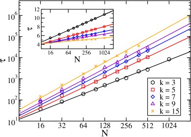
Figure 6: (Color online) Numerical results (full dots) for the freezing time $\tau$ as a function of the system size $N$ and for various $k$ [ $k=3$ (black circles) , $k=5$ (red squares) , $k=7$ (blue diamonds) , $k=9$ (violet triangles) and $k=15$ (orange crosses) ]. Each point is given by the average value over several realizations [ $100$ realizations for sizes $N\leq 64$ , $50$ realizations for $64<N\leq 256$ and $10$ realizations for $N>256$ ]. Moreover as initial configuration of each realization the links are chosen all negative ($\rho_{0}=0$, antagonistic society) in order to reduce the statistical error (the standard deviation is comparable with the symbol size) caused by the small number of realizations at larger sizes of the system. The full lines have slope $2(k-1)/k$ as expected from Eq.(37). The inset shows the numerical results for the freezing time $\tau$ , for different values of $k$ (the same as in the main plot), as a function of the system size $N$ and for $p=3/4$. Each point of the inset is given by the average over $10^{3}$ different realizations with initial antagonistic society.

For $p>1/2$ the freezing time $\tau$ scales as

$$\tau\sim\ln{N}\;\;\;.$$ (38)

The derivation would be the same as in the paper of Antal et al. antal . It should be noticed that for $p>1/2$ the paradise is reached as soon as $k$ increases. For simplicity let $p=1$ and imagine that the system is at the closest configuration to the paradise, for which only one link in the system has negative spin. This link belongs to $R=(N-2)!/(N-k)!$ different $k$-cycles. At each update event we select one $k$-cycle at random out of $M={N\choose k}$ total $k$-cycles. This way we have to wait a number of update events $E\sim M/R$ until the paradise is reached, which leads to a freezing time $\tau\sim E/L$, with $L$ the total number of links independent on $k$, so that

$$\tau\sim\frac{1}{k!}\;\;\;.$$ (39)

For values of $1/2<p<1$ the $k$-dependence of $\tau$ should be weaker than the one in Eq.(39), but anyway $\tau$ should be a decreasing function of $k$. The inset of Figure 6 shows the numerical results obtained for $p=3/4$ as a function of the size of the system $N$. The freezing time $\tau$ is measured for different values of $k$. We plot the average value over $10^{3}$ different realizations with initial condition $\rho_{0}=0$.

III.3.2 Freezing time for even values of $k$

In the case of even values of $k$ and $p=1/2$ the master equation for the density of positive links [ Eq.(20) ] reads as $d\rho/dt=0$. Therefore, the density of friendly links, $\rho$, should be constant during time for an infinite large system. In finite size systems the dynamics is subjected to non-negligible fluctuations. This allows to understand the scaling features of the freezing time $\tau$ with the system size. The order of the fluctuations is $\sqrt{L}$ because the process is completely random as we have seen for the case odd values of $k$ and $p<1/2$. Differently from the latter case, for even values of $k$ and $p=1/2$ the system has no tendency to go to a fixed point determined by $p$ because $d\rho/dt=0$. We can view the dynamical system as a Markov chain, with discrete steps in time and state space, for which the transition probability for passing from a state with $L^{-}(t-1)$ negative at time $t-1$ to a state with $L^{-}(t)$ negative links at time $t$ is given by

$$\begin{array}[]{l}P\left[\;L^{-}(t)\;|\;L^{-}(t-1)\;\right]=\\ ={L\choose L^{-}(t)}\left(\frac{L-L^{-}(t-1)}{L}\right)^{L-L^{-}(t)}\left(\frac{L^{-}(t-1)}{L}\right)^{L^{-}(t)}\;\;\;.\end{array}$$ (40)

So that the probability of having $L^{-}(t)$ negative links at time $t$ is just a binomial distribution where the probability of having one negative link is given by $\frac{L^{-}(t-1)}{L}$, the density of negative links at time $t-1$. This includes both the randomness of the displacement of negative links and the absence of a particular fixed point dependent on $p$. The Markov process, with transition probability given by Eq.(40), is known under the name of the Wright-Fisher model wright from the context of biology. The Wright-Fisher model is a simple stochastic model for the reproduction of diploid organisms (diploid means that each organism has two genes, here named as “$-$” and “$+$”), it was proposed independently by R.A. Fisher and S. Wright at the beginning of the thirties wright . The population size of genes in an organism is fixed and equal to $L/2$ so that the total number of genes is $L$. Each organism lives only for one generation and dies after the offsprings are made. Each offspring receives two genes, each one selected with probability $1/2$ out of the two genes of a parent of which two are randomly selected from the population of the former generation. Now let us assume that there is a random initial configuration of positive and negative genes with a slight surplus of negative genes. The offspring generation selects its genes randomly from this pool and provides the pool for the next offspring generation. Since the pools get never refreshed by a new random configuration, the initial surplus of negative links gets amplified in each offspring generation until the whole population of genes is ”negative”. Actually the solution of the Wright-Fisher model is quite simple. The process always converges to a final state with $L^{-}=0$ [$L^{+}=L$] or $L^{-}=L$ [$L^{+}=0$], corresponding to our heaven and [hell] solutions for even values of $k$. The average value over several realizations of the same process depends on the initial density of friendly links $\rho_{0}$ according to

$$\langle L^{-}\rangle=\rho_{0}\delta(0)+(1-\rho_{0})\delta(L)\;\;\;,$$

where $\delta(x)=1$ for $x=0$ and $\delta(x)=0$ otherwise. Furthermore, on average, the number of negative links decays exponentially fast to one of the two extremal values

$$\langle L^{-}(t)\rangle\simeq L\left\{\begin{array}[]{l}e^{-t/L}\\ 1-e^{-t/L}\end{array}\right.\;\;\;.$$

with typical decay time

$$\tau\sim L\sim N^{2}\;\;\;.$$ (41)

This result is perfectly reproduced by the numerical data plotted in Figure 7. The main plot shows the average time needed to reach a balanced configuration as a function of the size of the system $N$ and for different values of $k$ [ $k=4$ (black circles) , $k=6$ (red squares) , $k=8$ (blue diamonds) and $k=12$ (violet crosses) ]. The averages are performed over different numbers of realizations depending on the size $N$ [ $1000$ realizations for sizes $N\leq 128$ , $500$ realizations for $128<N\leq 384$ and $50$ realizations for $N=384$ and $N=512$, and $10$ realizations for $N=1024$ ]. The dashed line in Figure 7 has, in the log-log plane, a slope equal to $2$, all numerical data fit very well with this line. Furthermore it should be noticed that there is no $k$-dependence of the freezing time $\tau$, as it is described by Eq.(40). This is reflected by the fact that $\tau$ is the same for all the values of $k$ considered in the numerical measurements.

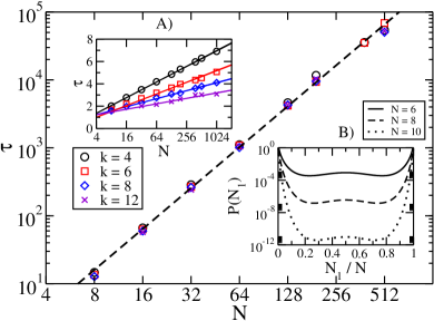
Figure 7: (Color online) Numerical results for the freezing time $\tau$ as a function of the system size $N$ and for various even values of $k$ [ $k=4$ (black circles) , $k=6$ (red squares) , $k=8$ (blue diamonds) and $k=12$ (violet crosses) ] and for $p=1/2$. Each point is given by the average value over several realizations [ $100$ realizations for sizes $N\leq 64$ , $50$ realizations for $64<N\leq 256$ and $10$ realizations for $N>256$ ]. Moreover, at the beginning of each realization the links are chosen to be positive or negative with the same probability ($\rho_{0}=0.5$). The dashed line has, in the log-log plane, slope $2$ as expected in Eq.(41). The inset A) shows the numerical results for the freezing time $\tau$ , for different values of $k$ (the same as in the main plot), as a function of the system size $N$ and for $p=3/4$. Each point of the inset is given by the average over $10^{3}$ different realizations with random initial conditions. The full lines are all proportional to $\ln{N}$ as expected. The inset B) shows the not-normalized probability $P(N_{1})$ as a function of the ratio $N_{1}/N$ and for different values of the system size $N$ [ $N=6$ (full line), $N=8$ (dashed line) and $N=10$ (dotted line) ]. As one can see, $P(N_{1})$ is extremely small for values of $0<N1<N$ already for $N=10$.

Nevertheless there is a difference between our model and the Wright-Fisher model that should be noticed. During the evolution of our model there is the possibility that the system freezes in a configuration different from the paradise ( $L^{-}=0$ ) or the hell ($L^{-}=L$ ). The probability of this event is still given by Eq.(23), with $r=L^{+}(N_{1})/L$ as the stationary condition [ $L^{+}(N_{1})$ is given by Eq.(21) ]. In this way Eq.(23) gives us $P(N_{1})$, the not-normalized probability for the system to freeze in a balanced configuration with two cliques of $N_{1}$ and $N-N_{1}$ nodes, respectively. It is straightforward to see that $P(N_{1})=1$ for $N_{1}=0$ or for $N_{1}=N$, so that the paradise has a non-vanishing probability to be a frozen configuration. Differently for any other value of $0<N_{1}<N$, $P(N_{1})$ decreases to zero faster than $1/N$. This means that for values of $N$ large enough it is appropriate to forget about the intermediate frozen configurations and to consider the features of our model as being very well approximated by those of the Wright-Fisher model. In the inset B) of Figure 7 the function $P(N_{1})$ is plotted for different values of $N$ [ $N=6$ (full line), $N=8$ (dashed line) and $N=10$ (dotted line) ] with $N_{1}$ a continuous variable for clarity of the figure (we approximate the factorial with the Stirling’s formula). Obviously $P(N_{1})$ disappears for $0<N_{1}<N$ as $N$ increases, already for reasonably small values of $N$.
The dependence $\tau\sim N^{2}$ can also be obtained using the same procedure as the one in section III.3.1 for the case odd values of $k$ and $p=1/2$. In particular for even values of $k$ we can rewrite Eq.(26) according to

$$A\longrightarrow\left\{\begin{array}[]{ll}A-1&\textrm{ , rate}\quad p\sum_{i=1}^{k/2}M_{2i-1}\\ A+1&\textrm{ , rate}\quad(1-p)\sum_{i=1}^{k/2}M_{2i-1}\end{array}\right.$$ (42)

and therefore Eq.(27) according to

$$A^{2}\longrightarrow\left\{\begin{array}[]{ll}A^{2}-2A+1&\textrm{ , rate}\quad p\sum_{i=1}^{k/2}M_{2i-1}\\ A^{2}+2A+1&\textrm{ , rate}\quad(1-p)\sum_{i=1}^{k/2}M_{2i-1}\end{array}\right.\;\;\;.$$ (43)

For $p=1/2$ we have

$$\frac{d\langle A\rangle}{dt}=0$$ (44)

and

$$\frac{d\langle A^{2}\rangle}{dt}=\sum_{i=1}^{k/2}\langle M_{2i-1}\rangle\;\;\;.$$

Eq.(44) tells us that $a\sim\langle A\rangle=$const, so that we have

$$\eta\sim\sqrt{t}\;\;\;,$$

remebering Eq.(34). As in the previous case, for determining the freezing time we impose the condition that the average value is of the same order as the fluctuations [Eq.(35)], and, for $L\sim N^{2}$, we obtain again Eq.(41).

For even values of $k$ and for $p\neq 1/2$ the time $\tau$ needed for reaching a frozen configuration scales as $\tau\sim\ln{N}$. In the inset of Figure 7 numerical estimates of $\tau$ for $p=3/4$ and different values of $k$ demonstrate this dependence on the size $N$ of the system. Each point is obtained from averaging over $10^{3}$ different simulations with the same initial conditions $\rho_{0}=0.5$. Again, as in the case of $k$ odd and $p>1/2$, $\tau$ is a decreasing function of $k$ and the same argument used for obtaining Eq.(39) can be applied here.

IV Diluted Networks

In this section we extend the former results, valid in the case of fully connected networks, to diluted networks. Real networks, apart from very small ones, cannot be represented by complete graphs. The situation in which all individuals know each other is in practice very unlikely. As mentioned in the introduction, links may be also missing, because individuals neither like nor dislike each other but are just indifferent. In the following we analyze the features of dynamical systems, still following the unconstrained $k$-cycle dynamics, but living on topologies given by diluted networks.
For diluted networks there is an interesting connection to another set of problems that leads to a new interpretation of the social balance problem in terms of a certain $k$-SAT ($k$S) problems (SAT stands for satisfiability) cook ; mezard ; mezard2 . In such a problem a formula $F$ consists of $Q$ logical clauses $\left\{C_{q}\right\}_{q=1,\ldots,Q}$ which are defined over a set of $B$ Boolean variables $\left\{x_{i}=0,1\right\}_{i=1,\ldots,B}$ which can take two possible values $0=$FALSE or $1=$TRUE. Every clause contains $k$ randomly chosen Boolean variables that are connected by logical $OR$ operations ($\bigvee$). They appear negated with a certain probability. In the formula $F$, all clauses are connected by logical $AND$ operations ($\bigwedge$)

$$F=\bigwedge_{q=1}^{Q}C_{q}\;\;\;,$$

so that all clauses $C_{q}$ should be simultaneously satisfied in order to satisfy the formula $F$. A particular formulation of the $k$S problem is the $k$-XOR-SAT ($k$XS) problem weigt ; semerjian ; mezard2 ; cocco , in which each clause $C_{q}$ is a parity check of the kind

$$C_{q}=x_{i_{1}}^{q}+x_{i_{2}}^{q}+\ldots+x_{i_{k}}^{q}\;\;\;\textrm{mod }2\;\;\;,$$ (45)

so that $C_{q}$ is TRUE if the total number of true variables which define the clause is odd, while otherwise the clause $C_{q}$ is FALSE. It is straightforward to map the $k$XS problem to our former model for the case odd values of $k$. Actually, each clause $C_{q}$ corresponds to a $k$-cycle [$Q\equiv M$] and each variable $x_{v}$ to a link $(i,j)$. Furthermore [$B\equiv L$] with the correspondence $s_{i,j}=1$ for $x_{v}=1$, while $s_{i,j}=-1$ for $x_{v}=0$. For the case of even values of $k$, one can use the same mapping but consider as clause $C_{q}$ in Eq.(45) its negation $\overline{C_{q}}$. In this way, when the number of satisfied variables $x_{i}^{q}$ is odd the clause $\overline{C_{q}}$ is unsatisfied for odd values of $k$, while $\overline{C_{q}}$ is satisfied for even values of $k$.
Moreover a typical algorithm for finding a solution of the $k$S problem is the so-called Random-Walk SAT (RWS). The procedure is the following weigt ; semerjian : select one unsatisfied clause $C_{q}$ randomly, next invert one randomly chosen variable of its $k$ variables $x_{i^{*}}^{q}$; repeat this procedure until no unsatisfied clauses are left in the problem. Each update is counted as $1/B$ units of time. As one can easily see, this algorithm is very similar to our unconstrained dynamics apart from two aspects. First, in our unconstrained dynamics we use the dynamical propensity parameter $p$, while it is absent in the RWS. Second, in our unconstrained dynamics we count also the choice of a balanced $k$-cycle as update event, although it does not change the system at all. Because of this reason, the literal application of the original algorithm of unconstrained dynamics has very high computational costs if it is applied to diluted networks. Apart from the parameter $p$, we can therefore use the same RWS algorithm for our unconstrained dynamics of $k$-cycles. This algorithm is more reasonable because it selects at each update event only imbalanced $k$-cycles which are actually the only ones that should be updated. In case of an all-to-all topology there are so many triads that a preordering according to the property of being balanced or not is too time consuming so that in this case our former version is more appropriate. In order to count the time as in our original framework of the unconstrained dynamics, we should impose that, at the $n$-th update event, the time increases as

$$t_{n}\;\;=\;\;t_{n-1}\;\;+\;\;\frac{1}{L}\;\cdot\;\frac{\alpha}{\alpha^{(n-1)}_{u}}\;\;\;.$$ (46)

Here $\alpha=M/L$ stands for the ratio of the total number of $k$-cycles of the system (i.e. total number of clauses) and the total number of links (i.e. total number of variables). The parameter $\alpha$ is called the “dilution” parameter, it can take all possible values in the interval $\left[0,{L\choose k}/L\right]$. $\alpha^{(n-1)}_{u}=\sum_{i=1}^{(k+1)/2}M_{2i-1}/L$ is the ratio of the total number of imbalanced (or “unsatisfied”) $k$-cycles over the total number of links, in particular $\alpha^{(n-1)}_{u}$ is computed before an instant of time at which the $n$-th update event is implemented. Therefore the ratio $\alpha/\alpha^{(n-1)}_{u}$ gives us the inverse of the probability for finding an imbalanced $k$-cycle, out of all, balanced or imbalanced, $k$-cycles, at the $n$-th update event. This is a good approximation to the time defined in the original unconstrained dynamics. It should be noticed that this algorithm works faster in units of this computational time, but the simulation time should be counted in the same units as defined for the unconstrained dynamics introduced in section II.
The usual performance of the RWS is fully determined by the dilution parameter $\alpha$. For $\alpha\leq\alpha_{d}$ the RWS always finds a solution of the $k$S problem within a time that scales linearly with the number of variables $L$. In particular for the $k$XS problem $\alpha_{d}=1/k$. For $\alpha_{d}<\alpha<\alpha_{c}$ the RWS is still able to find a solution for the $k$S problem, but the time needed to find the solution grows exponentially with the number of variables $L$. For the case of the $3$XS problem $\alpha_{c}\simeq 0.918$. $\alpha_{d}$ is the value of the dilution parameter for which we have the “dynamical” transition, depending on the dynamics of the algorithm while $\alpha_{c}$ represents the transition between the SAT and the UNSAT regions: for values of $\alpha\geq\alpha_{c}$ the RWS is no longer able to find any solution for the $k$S problem, and in fact no such solution with zero frustration exists for the $k$S problem. Furthermore there is a third critical threshold $\alpha_{s}$, with $\alpha_{d}<\alpha_{s}<\alpha_{c}$. For values of $\alpha<\alpha_{s}$ all solutions of the $k$S problem found by the RWS are located into a large cluster of solutions and the averaged and normalized Hamming distance inside this cluster is $\langle d\rangle\simeq 1/2$. For $\alpha>\alpha_{s}$ the solutions space splits into a number of small clusters (that grows exponentially with the number of variables $L$) , for which the averaged and normalized Hamming distance inside each cluster is $\langle d\rangle\simeq 0.14$, while the averaged and normalized Hamming distance between two solutions lying in different clusters is still $\langle d\rangle\simeq 1/2$ cocco . For the special case of the $3$XS problem $\alpha_{s}$ was found as $\alpha_{s}\simeq 0.818$.
In order to connect the problems of social balance on diluted networks and the $k$XS problem on a diluted system we shall first translate the parameters into each other. First of all we need to calculate the ratio $\alpha=M/L$ between the total number of $k$-cycles of the network and the total number of links $L$ (section IV.1). Next we consider the standard RWS applied to the $k$XS problem taking care of the right way of computing the time as it is given by the rule (46) and the introduction of the dynamical parameter $p$ (section IV.2). In particular we focus on the “dynamical” transition at $\alpha_{d}$ (section IV.2.1) and the transition in solution space concerning the clustering properties of the solutions at $\alpha_{s}$ (section IV.2.2). The dynamical parameter $p$, formerly called the propensity parameter, leads to a critical value $p_{c}$ above which it is always possible to find a solution within a time that grows at most linearly with the system size (section IV.2.3). Finally, in section IV.2.4 we decrease the dilution, i.e. increase $\alpha$ to $\alpha_{m}$ such that for $\alpha\geq\alpha_{m}$ the system is fully described by the mean field equations of the former sections. We focus on the simplest case $k=3$, but all results presented here for $k=3$ should be qualitatively valid for any value of $k\geq 3$.

IV.1 Ratio $\alpha$ for random networks

Let us first consider Erdös-Rényi networks erdos as a diluted version of the all-to-all topology that we studied so far. An Erdös-Rényi network, or a random network, is a network in which each of the ${N\choose 2}$ different pairs of nodes is connected with probability $w$. The average number of links is simply $\langle L\rangle=w{N\choose 2}$. The average number of cycles of order $k$ is given $\langle M\rangle=w^{k}{N\choose k}$, so that the average ratio $\langle\alpha\rangle$ can be estimated as

$$\langle\alpha\rangle\simeq w^{k-1}\frac{2N^{k-2}}{k!}\;\;\;.$$ (47)

In Figure 8 we plot the numerical results obtained for the ratio $\alpha$ as a function of the probability $w$, in the particular case of cycles of order $k=3$. The reported results, from bottom to top, have been obtained for values of $N=16,32,48,64,96,128,192$ and $256$. Each point is given by the average over $10^{3}$ different network realizations. In particular these numerical results fit very well with the expectations (full lines) of Eq.(47), especially for large values of $N$ and/or small values of $w$. Furthermore the critical values $\alpha_{d}=1/3$ , $\alpha_{s}=0.818$ and $\alpha_{c}=0.918$ (dotted lines) are used for extrapolating the numerical results of $w_{d}$ (open circles), $w_{s}$ (open squares) and $w_{c}$ (gray squares) respectively [see the inset of Figure 8]. $w_{i}\;,\;i=d,s,c$ is the value of the probability for which the ratio $\alpha_{i}\;,\;i=d,s,c$ is satisfied. As expected, they follow the rule $w_{i}=\sqrt{3\alpha_{i}/N}\;,\;i=d,s,c$ predicted by Eq.(47) for $k=3$.

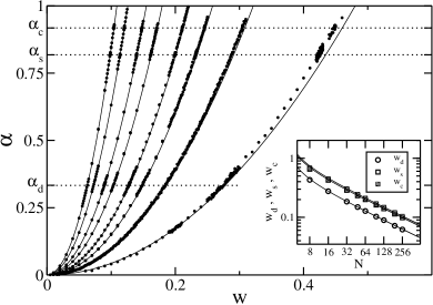
Figure 8: Numerical results (full dots) for the ratio $\alpha=M/L$ between the total number of cycles $M$ of order $k=3$ and the total number of links $L$ as a function of the probability $w$ for different sizes of Erdös-Rényi networks. In particular the numerical results refer to different network size $N$: from bottom to top $N=16,32,48,64,96,128,192$ and $256$. Each point is given by the average over $10^{3}$ network realizations. The full lines are the predicted values given by Eq.(47), while the dotted lines denote the critical values $\alpha_{d}=1/3$ , $\alpha_{s}=0.818$ and $\alpha_{c}=0.918$ as described in detail in the text. In particular the numerical values of the probability $w$ for which these three critical values of $\alpha$ are realized are denoted by $w_{d}$ (open circles), $w_{s}$ (open squares) and $w_{c}$ (gray squares) respectively, they are plotted in the inset, where the full lines are extrapolated by Eq.(47) as $w_{i}=\sqrt{3\alpha_{i}/N}\;,\;i=d,s,c$. The two upper curves for $w_{s}$ and $w_{c}$ almost coincide.

According to the isomorphism traced between the $k$XS problem and the social balance for $k$-cycles, from now on we will not make any distinction between the words problem and network, variable and link, $k$-clause and $k$-cycle, value and sign (or spin), false and negative (or unfriendly), true and positive (or friendly), satisfied and balanced (or unfrustrated), unsatisfied and imbalanced (or frustrated), etc….

IV.2 $p$-Random-Walk SAT

So far we have established the connection between the $k$XS problem and the social balance for $k$-cycles, proposed in this paper. In particular we have determined how the dilution parameter $\alpha$ is related to diluted random networks parameterized by $w$. In this section we extend the known results for the standard RWS of weigt ; semerjian to the $p$-Random-Walk SAT ($p$RWS) algorithm, that is the RWS algorithm extended by the dynamical parameter $p$ that played the role of a propensity parameter in connection with the social balance problem. The steps of the $p$RWS are as follows:

1. Select randomly a frustrated clause between all frustrated clauses.

2. Instead of randomly inverting the value of one of its $k$ variables, as for an update in the case of the RWS, apply the following procedure:

   • if the clause contains both true and false variables, select with probability $p$ one of its false variable, randomly chosen between all the false variables belonging to the clause, and flip it to the true value;

   • if the clause contains both true and false variables, select with probability $1-p$ one of its true variable, randomly chosen between all the true variables belonging to the clause, and flip it to the false value;

   • if the clause contains only false values ($k$ should be odd), select with probability $1$ one of its false variables, randomly chosen between all the false variables belonging to the clause, and flip it to the true value.

3. Go back to point 1 until no unsatisfied clauses are present in the problem.

The update rules of point 2 are the same used in the case of $k$-cycle dynamics and illustrated in Figure 1 for the cases $k=4$ (A) and $k=5$ (B). For the special case of $3$XS problem, the standard RWS algorithm and the $p$RWS algorithm coincides for the dynamical parameter $p=1/3$.

IV.2.1 Dynamical transition at $\alpha_{d}$

The freezing time $\tau$, that is the time $\tau$ needed for finding a solution of the problem, abruptly changes its behavior at the dynamical critical point $\alpha_{d}=1/k$.
Figure 9 reports the numerical estimate of the freezing time $\tau$ as a function of the dilution parameter $\alpha$ and for different values of the dynamical parameter $p$ [ $p=0$ (circles) , $p=1/3$ (squares) , $p=1/2$ (diamonds) and $p=1$ (crosses) ]. As one can easily see, for $p=1/3$ and $p=0$, $\tau$ drastically changes around $\alpha_{d}$, increasing abruptly for values of $\alpha>\alpha_{d}$. For $p=1/2$ and for $p=1$ this drastic change is not observed. This is understandable from the fact that both values of $p$ provide a bias towards paradise, while $p=1/3$ corresponds to a random selection of one of the three links of a triad as in the original RWS and $p=0$ would favor the approach to the hell if it were a balanced state. The simulations are performed over a system with $L=10^{3}$ variables. Moreover each point stands for the average over $10^{2}$ different networks and $10^{2}$ different realizations of the dynamics on such topologies. At the beginning of each simulation the variables take the value $1$ or $0$ with the same probability. The inset shows the relation between the time $\tau^{*}$ calculated using the standard RWS and the time $\tau$ calculated according to Eq.(46). The almost linear relation (the dashed line has a slope equal to one) between $\tau^{*}$ and $\tau$ means that there is no qualitative change between the two different ways of counting the time.

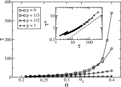
Figure 9: Time $\tau$ for reaching a solution for a system of $L=1000$ variables as a function of the ratio $\alpha$ and for different values of the dynamical parameter $p$ [ $p=0$ (circles), $p=1/3$ (squares), $p=1/2$ (diamonds) and $p=1$ (crosses) ]. The $p$RWS performed for $p=1/3$ shows a critical behavior around $\alpha_{s}=1/3$: for values of $\alpha\leq\alpha_{s}$, $\tau$ grows almost linearly with $\alpha$, while it jumps to an exponential growth with $\alpha$ for $\alpha>\alpha_{s}$. The same is qualitatively true for $p=0$, but the time $\tau$ needed for reaching a solution increases more slowly with respect to the case $p=1/3$ for $\alpha>\alpha_{s}$. For $p=1/2$ and $p=1$ there seems to be no drastic increment of $\tau$ for $\alpha>\alpha_{s}$. Moreover the inset shows the dependence of $\tau^{*}$, the freezing time as calculated in the standard RWS weigt ; semerjian , on the freezing time $\tau$ calculated according to Eq.(46). The almost linear dependence of $\tau^{*}$ on $\tau$ (the dashed line has slope one) explains that there is no qualitative change if we describe the dynamical features of the system in terms of $\tau$ or $\tau^{*}$ as time used by the simulations.

Following the same argument as in weigt , we can specify for the update event at time $t$ the variation of the number of unsatisfied clauses $M_{t}^{(u)}$ as

$$\Delta M_{t}^{(u)}=-\left(k\alpha_{u}(t)+1\right)+k\alpha_{s}(t)=k\alpha-2k\alpha_{u}(t)-1\;\;\;,$$

because, by flipping one variable of an unsatisfied clause, all the other unsatisfied clauses which share the same variable become satisfied, while all the satisfied clauses containing that variable become unsatisfied. In the thermodynamic limit $L\to\infty$, one can impose $M_{t}^{(u)}=L\alpha_{u}(t)$. Moreover, the amount of time of one update event is given by Eq.(46) so that we can write

$$\dot{\alpha}_{u}(t)=\frac{\alpha_{u}(t)}{\alpha}\left(k\alpha-2k\alpha_{u}(t)-1\right)\;\;\;.$$ (48)

Eq.(48) has as stationary state (or a plateau) at

$$\alpha_{u}=\frac{k\alpha-1}{2k}\;\;\;.$$ (49)

Therefore, when the ratio $\alpha$ (that is the ratio of the number of clauses over the number of variables) exceeds the critical “dynamical” value

$$\alpha_{d}=\frac{1}{k}\;\;\;,$$ (50)

the possibility of finding a solution for the problem drastically changes. This result was already found by weigt ; semerjian . While for values of $\alpha\leq\alpha_{d}$ we can always find a solution because the plateau of Eq.(49) is always smaller or equal to zero, for $\alpha>\alpha_{d}$ the solution is reachable only if the system performs a fluctuation large enough to reach zero from the non-zero plateau of Eq.(49). In Figure 10 we report some numerical simulations for $\alpha_{u}$ as a function of the time for different values of $p$ [ A) $p=0$ , B) $p=1/3$ , C) $p=1/2$ , D) $p=1$ ] and for different values of the dilution parameter $\alpha$ [ $\alpha=0.3$ (black, bottom) , $\alpha=0.5$ (red, middle) , $\alpha=0.85$ (blue, top) ]. The numerical values [full lines] are compared with the numerical integration of Eq.(48) [dashed lines]. They fit very well apart from large values of $t$, for $\alpha=0.85$ and for $p=1/2$ or $p=1$. The initial configuration in all cases is that of an antagonistic society ($x_{i}=0\;\;\;,\;\forall\;i=1,\ldots,L$), while the number of variables is $L=10^{4}$.

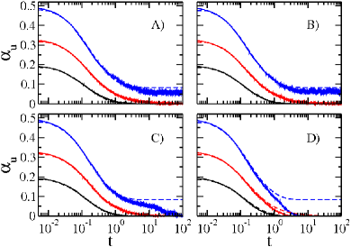
Figure 10: (Color online) Time behavior of the ratio $\alpha_{u}$ of unsatisfied clauses for different values of $p$ [ A) $p=0$ , B) $p=1/3$ , C) $p=1/2$ , D) $p=1$ ] and for different values of the dilution parameter $\alpha$ [ $\alpha=0.3$ (black, bottom) , $\alpha=0.5$ (red, middle) , $\alpha=0.85$ (blue, top) ]. Numerical results of simulations [full lines] are compared with the numerical integration of Eq.(48) [dashed lines] leading to a very good fit in all cases, except for $\alpha=0.85$ and for $p=1/2$ and $p=1$. The initial configuration in all the cases is the one of an antagonistic society ($x_{i}=0\;\;\;,\;\forall\;i=1,\ldots,L$), while the number of variables is $L=10^{4}$.

IV.2.2 Clustering of solutions at $\alpha_{s}$

In order to study the transition in the clustering structure of solutions at $\alpha_{s}$, we numerically determine the Hamming distance between different solutions of the same problem. More precisely, given a problem of $L$ variables and $M$ clauses, we find $T$ solutions $\left\{x_{i}^{r}\right\}_{i=1,\ldots,L}^{r=1,\ldots,T}$ of the given problem. This means that we start $T$ times from a random initial configuration and at each time we perform a $p$RWS until we end up with a solution. We then compute the distance between these $T$ solutions as normalized Hamming distance

$$\langle d\rangle=\frac{1}{L\cdot T(T-1)}\sum_{r,s=1}^{T}\sum_{i=1}^{L}\left|x_{i}^{r}-x_{i}^{s}\right|\;\;\;.$$ (51)

The numerical results for $L=20$ are reported in Figure 11. We average the distance over $T=10^{2}$ trials and over $10^{2}$ different problems for each value of $\alpha$. As expected for $p=1/3$ [squares] the distance between solutions drops down around $\alpha_{s}$ (actually it drops down before $\alpha_{s}$ because of the small number of variables). For different values of $p$ [ $p=0$ (circles) , $p=1/2$ (diamonds) and $p=1$ (crosses) ], the $p$RWS is less random and $\langle d\rangle$ drops down before $\alpha_{s}$ (or at least before the point at which the case $p=1/3$ drops down). In particular, if we plot (as in the inset) the distance $\langle d\rangle$ as a function of $p$ and for different values of $\alpha$ [$\alpha=0.3$ (full line) , $\alpha=0.5$ (dotted line) and $\alpha=0.85$ (dashed line)] we see a clear peak of the distance $\langle d\rangle$ around $p=1/3$. This suggests that a completely random, unbiased RWS always explores a large region in phase space, it leads to a larger variety of solutions.

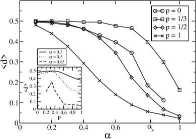
Figure 11: Normalized Hamming distance $\langle d\rangle$ [ Eq.(51) ] between solutions as a function of the ratio $\alpha$ and different values of the dynamical parameter $p$ [ $p=0$ (circles) , $p=1/3$ (squares) , $p=1/2$ (diamonds) and $p=1$ (crosses)]. For the standard RWS ($p=1/3$) the distance drops down around the critical point $\alpha_{s}$. Different values of $p$ perform not-really random walks and lead to effective values of $\alpha_{s}$ smaller than the former one. The inset shows the dependence of $\langle d\rangle$ on the dynamical parameter $p$. As it is shown for different values of $\alpha$ [$\alpha=0.3$ (full line) , $\alpha=0.5$ (dotted line) and $\alpha=0.85$ (dashed line)] the peak of the distance between solutions is for a $p$RWS which is really random, that is for $p=1/3$. All the points here , in the main plot as well as in the inset, are obtained for a system of $L=20$ variables. Each point is obtained averaging over $10^{2}$ different networks and on each of these networks the average distance is calculated over $10^{2}$ solutions. At the beginning of each simulation the value of one variable is chosen to be $1$ or $0$ with equal probability.

IV.2.3 SAT/UNSAT transition at $\alpha_{c}$

Differently from the general $k$S problem, the $k$XS problem is known to be always solvable semerjian and the solution corresponds to one of the balanced configurations as described in section III.3 for the all-to-all topology. Nevertheless the challenge is whether the solutions can be found by a local random algorithm like RWS. In the application of the RWS it can happen that the algorithm is not able to find one of these solutions in a “finite” time, so that the problem is called “unsatisfied”. The notion is made more precise in cocco . For practical reasons the way of estimating the critical point $\alpha_{c}$ that separates the SAT from the UNSAT region is related to the so-called algorithm complexity of the RWS. Here we follow the prescription of weigt ; semerjian ; schoning . Fixed $k=3$ and calling a RWS with initial random assignment of the variables followed by $3L$ update events one trial, one needs a total number of trials $T\gg\left(4/3\right)^{L}$ for being “numerically” sure to be in the UNSAT region. In fact if after $T$ trials no solution is found, the problem is considered as “unsatisfied” .
The introduction of the dynamical parameter $p$ can strongly “improve” the performance of RWS. For $p\neq 1/3$ the $p$RWS updates the variables following a well prescribed direction: the tendency is to increases the number of negative variables for $p<1/3$ and to decrease their number for $p>1/3$. In particular, as we have seen in the former sections, for $p\geq 1/2$ the $p$RWS approaches the configuration of the paradise for the largest value of $\alpha={L\choose k}/L\gg\alpha_{c}$ and in a time that goes as $\tau\sim L^{\beta}$, so that there is no UNSAT region at all if we apply the former criterion for the numerical estimate of the UNSAT region. Clearly, if the bias goes in the wrong direction, the performance gets worse.
In this section we briefly give a qualitative description about the SAT/UNSAT region for the $p$RWS due to the dynamical parameter $p$. Let us define as ${}^{+}p_{c}$ [${}^{-}p_{c}$] the minimum [maximum] value of $p$ for which the system can be satisfied. Given a problem with $\alpha L$ clauses we follow the algorithm: 1) Set $p=1$ [$p=0$] ; 2) set an initial random configuration and apply the $p$RWS ; 3) if the $p$RWS finds the solution in a number of updates less than $U\cdot L$ , decrease [increase] $p$ and go to point 2) ; 4) if not ${}^{+}p_{c}=p$ [${}^{-}p_{c}=p$]. This procedure can be performed up to the desired sensitivity for the numerical estimate of ${}^{+}p_{c}$ [${}^{-}p_{c}$]. The idea of defining an upper ${}^{+}p_{c}$ and lower critical value ${}^{-}p_{c}$ for the dynamical parameter $p$ is related to the fact that for $p=1/3$ the $p$RWS has most trouble to find the solution. Figure 12B and Figure 12C show the numerical results for ${}^{+}p_{c}$ and ${}^{-}p_{c}$ as a function of the dilution parameter $\alpha$. The number of variables is $L=10^{3}$. We report the results for different values of the waiting time $T=L\cdot U$ [ $U=1$ (circles) , $U=2$ (squares) , $U=3$ (crosses) , $U=10$ (crosses) ]. Each point is averaged over $10$ different problems and $10$ different $p$RWS applied to each problem. Qualitatively it is seen that for $\alpha\leq\alpha_{d}$ the problem is always solvable ( ${}^{+}p_{c}=0$ and ${}^{-}p_{c}=1$ ) , while for $\alpha>\alpha_{d}$ one needs $p\neq 1/3$ for solving the problem. Of course the numerical values for ${}^{+}p_{c}$ and ${}^{-}p_{c}$ depend on the waiting time until the $p$RWS reaches a solution. Here, for simplicity we do not wait long enough for seeing a similar behavior around $\alpha_{c}$ instead of $\alpha_{d}$. Furthermore, in Figure 12A we report the probability $P$, that is the ratio of success over the number of trials, for solving the problem as a function of $p$ for $\alpha=\alpha_{c}$. The waiting time is $U=1$ (circles) , $U=2$ (squares) , $U=3$ (diamonds) , $U=10$ (crosses) and $U=100$ (triangles), respectively. The probabilities are calculated over $10^{2}$ trials for each point ($10$ different problems times $10$ $p$RWS for each problem). As the waiting time increases the upper critical value ${}^{+}p_{c}$ for finding for sure the solution decreases ( ${}^{+}p_{c}\simeq 0.8$ for $U=1$ , ${}^{+}p_{c}\simeq 0.7$ for $U=2$ , ${}^{+}p_{c}\simeq 0.6$ for $U=3$ and for $U=10$ , ${}^{+}p_{c}\simeq 0.5$ for $U=100$ ). This means that even for less biased search, solutions can be found, while ${}^{-}p_{c}$ is zero for the waiting time reported here, no value of $p<p_{c}$ leads to a solution. This is as expected. If the variables are almost all negative it is harder to find a solution of the problem (the paradise is a solution while the hell for $k$ odd is not).

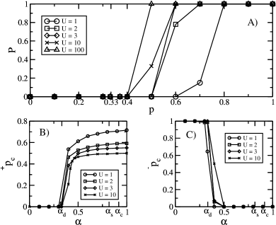
Figure 12: Numerical estimate of the upper ${}^{+}p_{c}$ (B) and lower ${}^{-}p_{c}$ (C) critical values of $p$ [see the text for their definition] as a function of the dilution parameter $\alpha$. Here $L=10^{3}$ and the different symbols corresponds to different maximum waiting times $T=U\cdot L$ [ $U=1$ (circles) , $U=2$ (squares) , $U=3$ (diamonds) , $U=10$ (diamonds) ]. Each point is given by the average over $10$ different problems for each value of $\alpha$ and $10$ different $p$RWS for each problem (with random initial condition). Moreover in (A) we show the probability $P$ that the $p$RWS finds a solution at $\alpha=0.918\simeq\alpha_{c}$ as a function of $p$. We used different waiting times [ $U=1$ (circles) , $U=2$ (squares) , $U=3$ (diamonds) , $U=10$ (crosses) , $U=100$ (triangles) ]. See the text for further comments.

IV.2.4 Mean-field approximation down to $\alpha_{m}$

By construction the “topology” of a $k$S problem is completely random (for this reason is sometimes called explicitly as Random $k$-SAT problem). Each of the $L$ variables can appear in one of the $\alpha L$ clauses with probability $v=\frac{1}{L}+\frac{1}{L-1}+\ldots+\frac{1}{L-k}$. In particular for $L\gg k$ one can simply write $v\simeq\frac{k}{L}$. Then the probability $P_{r}$ that one variable belongs to $r$ clauses can be described by the Poisson distribution

$$P_{r}=\frac{\left(\alpha k\right)^{r}}{r!}e^{-\alpha k}\;\;\;,$$ (52)

with mean value $\langle r\rangle=\alpha k$ and variance $\sigma_{r}=\sqrt{\alpha k}$. $P_{r}$ is plotted in Figure 13, where the numerical results [ symbols , $r=0$ (black circles) , $r=1$ (red squares) , $r=2$ (blue diamonds) and $r\geq 3$ (violet crosses) ] are compared to the analytical expectation [ lines , $r=0$ (black full line) , $r=1$ (red dotted line) , $r=2$ (blue dashed line) and $r\geq 3$ (violet dotted-dashed line) ].

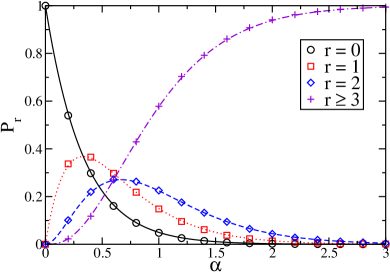
Figure 13: Probability $p_{r}$ that one variable belongs to $r$ clauses as function of the dilution parameter $\alpha$. The symbols stand for numerical results obtained over $10^{3}$ different realizations for $L=128$ variables [ $r=0$ (black circles) , $r=1$ (red squares) , $r=2$ (blue diamonds) and $r\geq 3$ (violet crosses) ]. The lines stand for analytical predictions of Eq.(52) [ $r=0$ (black full line) , $r=1$ (red dotted line) , $r=2$ (blue dashed line) and $r\geq 3$ (violet dotted-dashed line) ].

If we start from an antagonistic society (all variables false) the minimum value of the dilution $\alpha_{m}$ needed to reach the paradise (if $p\geq 1/2$) is that all variables belong to at least one clause. This means that $P_{0}<1/L$, from which

$$\alpha_{m}=\frac{\ln{L}}{k}\;\;\;.$$ (53)

It is interesting to note that the same criterion applies for any $p$. In Figure 14 we plot the absolute value of the difference $\left|\;{}^{(m)}\rho_{\infty}-\;^{(t)}\rho_{\infty}\;\right|$, between ${}^{(t)}\rho_{\infty}$, the theoretical prediction for the stationary density of true variables, [ Eq.(14) ] and the numerically measured value ${}^{(m)}\rho_{\infty}$, as a function of the dilution parameter $\alpha$. ${}^{(m)}\rho_{\infty}$ is obtained as the average of the density of friendly links (registered after a waiting time $T=200.0$ , so that is effectively the stationary density) over $50$ different problems and $50$ different $p$RWS for each problem. The results reported here are for $L=128$ (open symbols) and $L=256$ (gray filled symbols) and for different values of $p$ [ $p=0$ (circles) , $p=1/3$ (squares) , $p=1/2$ (diamonds) , $p=1$ (triangles) ]. The initial conditions are those of an antagonistic society. The dashed lines are proportional to $e^{-3\alpha}$. Figure 14 shows that the mean-field approximation of Eq.(14) becomes exponentially fast true as the system dilution decreases. Moreover, as for the cases $p=0$ and $p=1/3$, we can observe that the difference $\left|\;{}^{(m)}\rho_{\infty}-\;^{(t)}\rho_{\infty}\;\right|$ is always smaller than for $p=1/2$ and $p=1$. Qualitatively this means that the dilution $\alpha$ of the system needed to reach the theoretical expectation of Eq.(14) is smaller than $\alpha_{m}$ for $p<1/2$. In general we can say that $\alpha_{m}$ is a function of $p$: $\alpha_{m}=\alpha_{m}(p)$, and $\alpha_{m}$ is the minimum value of the dilution of the system for which we can effectively describe the diluted system as an all-to-all system for all the values of $p$. Moreover, it should be noticed that for $\alpha>\alpha_{m}$ almost all variables belong to at least three clauses [ see Figure 13 ]. This fact allows the $p$RWS to explore a larger part of configuration space. Let us assume that one variable belongs to less than three clauses: an eventual update event that flips this variable so that the one triad becomes balanced, can never increase the number of unsatisfied clauses by frustrating other clauses it belongs to. This reminds us to the situation in an energy landscape in which an algorithm gets stuck in a local minimum when it never accepts a change in the “wrong” direction, i.e. towards larger energy.

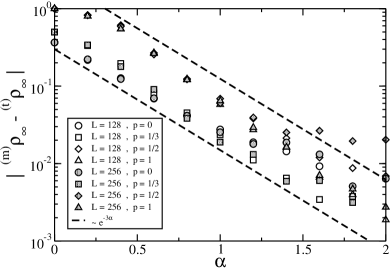
Figure 14: Difference $\left|\;{}^{(m)}\rho_{\infty}-\;^{(t)}\rho_{\infty}\;\right|$ between ${}^{(t)}\rho_{\infty}$ the theoretical prediction for the stationary density of friendly variables [ Eq.(14) ] and the numerically measured value ${}^{(m)}\rho_{\infty}$, as a function of the dilution parameter $\alpha$. ${}^{(m)}\rho_{\infty}$ is obtained as the average of the density of friendly links (registered after a waiting time $T=200.0$ , so that is effectively stationary ) over $50$ different problems and $50$ different $p$RWS for each problem. The results displayed here are obtained for $L=128$ (open symbols) and $L=256$ (gray filled symbols) and for different values of $p$ [ $p=0$ (circles) , $p=1/3$ (squares) , $p=1/2$ (diamonds) , $p=1$ (triangles) ]. The initial conditions are those of an antagonistic society. The dashed lines are proportional to $e^{-3\alpha}$.

V Summary and conclusions

In the first part of this paper we generalized the triad dynamics of Antal et al. to a $k$-cycle dynamics antal . Here we had to distinguish the cases of even values of $k$ and odd values of $k$. For all values of integer $k$ there is again a critical threshold at $p_{c}=1/2$ in the propensity parameter. For odd $k$ and $p<p_{c}$ the paradise can never be reached in the thermodynamic limit of infinite system size (as predicted by the mean field equations which we solved exactly for $k=5$ and approximately for $k>5$). In the finite volume, in principle one could reach a balanced state made out of two cliques (a special case of this configuration is the “paradise” when one clique is empty). However, the probability for reaching such type of frozen state decreases exponentially with the system size so that in practice the fluctuations never die out in the numerical simulations. For $p>1/2$ the convergence time to reach the paradise grows logarithmically with the system size. At $p=1/2$ paradise is reached within a time that follows a power law in the size $N$, where we determined the $k$-dependence of the exponent. In particular, the densities of $k$-cycles with $j$ negative links, here evolved according to the rules of the $k$-cycle dynamics, could be equally well obtained from a random dynamics in which each link is set equal to $1$ with probability $\rho_{\infty}$ or equal to $-1$ with probability $1-\rho_{\infty}$. This feature was already observed by Antal et al. for $k=3$ antal . It means that the individual updating rules which seem to be “socially” motivated in locally reducing the social tensions by changing links to friendly ones, end up with random distributions of friendly links. The reason is a missing constraint of the type that the overall number of frustrated $k$-cycles should not increase in an update event. Such a constrained dynamics was studied by Antal et al. in antal , but not in this paper.
For even values of $k$, the only stable solutions are “heaven” (i.e. paradise) and “hell” for $p>1/2$ and $p<1/2$, respectively, and the time to reach these frozen configurations grows logarithmically with $N$. At $p_{c}=1/2$ other realizations of the frozen configurations are possible, in principle. However, they have negligible probability as compared to heaven and hell. Here the time to reach these configurations increases quadratically in $N$, independently of $k$. This result was obtained in two ways. Either from the criterion to reach the stable state when a large enough fluctuation drops the system into this state (so we had to calculate how long one has to wait for such a big fluctuation). Alternatively, the result could be read off from a mapping to a Markov process for diploid organisms ending up in a genetic pool of either all “$+$”-genes or all “$-$”-genes. The difference in the possible stable states of diploid organisms and ours consists in two-clique stable solutions that are admissible for the even $k$-cycle dynamics, in principle, however such clique states have such a low probability of being realized that the difference is irrelevant.
The difference in the exponent at $p_{c}$ and the stable configurations above and below $p_{c}$ between the even and odd $k$-cycle dynamics was due to the fact that ”hell”, a state with all links negative as in an antagonistic society, is a balanced state for even $k$, not only by the frustration criterion of physicists, but also according to the criterion of social scientists cartwright .

As a second natural generalization of the social balance dynamics of Antal et al. we considered a diluted network. One way of implementing the dilution is via a random Erdös-Rényi network, characterized by the probability $w$ for connecting a randomly chosen pair of nodes. Here we focused our studies to the case $k=3$. The mean-field description and the results about the phase structure remain valid down to a certain degree of dilution, characterized by $w_{m}$. This threshold for the validity of the mean-field description practically coincides with the criterion whether a single link belongs to at least three triads (for $w>w_{m}$) or not ($w<w_{m}$). If it does so, an update event can increase the number of frustrated triads. For $w<w_{m}$, or more precisely $w<w_{d}<w_{m}$ it becomes easier to realize frozen configurations different from the paradise. Isolated links do not get updated at all and isolated triads can freeze to a “$+$”-“$-$”-configuration. The time to reach such a frozen configuration (in general different from the paradise) grows then only linearly in the system size. Also the solution space, characterized by the average Hamming distance between solutions, has different features below and above another threshold, called $w_{s}$ with $w_{d}<w_{s}<w_{m}$. Therefore one of the main differences between the all-to-all and the sufficiently diluted topology are the frozen configurations. For the all-to-all case we observed the paradise above $p_{c}$ for odd values of $k$ and even values of $k$ and the hell for even values of $k$ below $p_{c}$, in the numerical simulations, because the probability to find a two-clique-frozen configuration was calculated to be negligibly small. For larger dilution, also other balanced configurations were numerically found, as mentioned above, and the time passed in the numerical simulations for finding these solutions followed the theoretical predictions.
In section IV we used, however, another parameterization in terms of the dilution parameter $\alpha$, that was the ratio of triads (clauses) over the number of links [we gave anyway an approximated relation between $\alpha$ and $w$ in Eq.(47)]. The reason for using this parameterization was a mapping of the $k$-cycle social balance of networks to a $k$-XOR-SAT ($k$XS) problem, that is a typical satisfiability problem in optimization tasks. We also traced a mapping between the “social” dynamical rules and the Random-Walk SAT (RWS) algorithm, that is one approach for solving this problem in a random local way. As we have shown, the diluted version of the $3$-cycle social dynamics with propensity parameter $p=1/3$ corresponds to a $3$XS problem solved by the RWS algorithm in its standard form (as used in weigt ; semerjian ).
The $k$XS problem is always solvable like the $k$-cycle social balance, for which a two cliques solution always exists due to the structure theorem of cartwright , containing as a special solution the so-called paradise. The common challenge, however, is to find this solution by a local stochastic algorithm. The driving force, shared by both sets of problems, is the reduction of frustration. The meaning of frustration depends on the context: for the $k$-cycle dynamics it is meant in a social sense as a reduction of social tension, for the $k$XS problem it corresponds to violated clauses. The mathematical criterion is the same. The local stochastic algorithm works in a certain parameter range, but outside this range it fails. The paradise is never reached for a propensity parameter $p<1/2$, independently of $k$. Similarly, the solution of the $k$XS problem is never found if the dilution parameter is larger than $\alpha_{c}$, and the RWS algorithm needs an exponentially long time already for $\alpha>\alpha_{d}$, with $\alpha_{d}<\alpha_{c}$.
We generalized the RWS algorithm, usually chosen for solving the $k$-SAT ($k$S) problem as well as the $k$XS problem, to include a parameter $p$ that played formerly the role of the propensity parameter in the social dynamics ($p$RWS). The effect of this parameter is a bias towards the solution so that $\alpha_{d}$, the threshold between a linear and an exponential time for solving the problem, becomes a function of $p$. Problems for which the $p$RWS algorithm needed exponentially long for $p=1/3$, now become solvable within a time that grows less than logarithmically in the system size for $p>1/2$ and less than power-like in the system size for $p=1/2$. Along with the bias goes an exploration of solution space that has on average a smaller Hamming distance between different solutions than in the case of the $\frac{1}{3}$RWS algorithm that was formerly considered weigt ; semerjian .

Our paper has illustrated that the reduction of frustration may be the driving force in common to a number of dynamical systems. So far we were concerned about “artificial” systems like social systems and satisfiability problems. It would be interesting to search for natural networks whose evolution was determined by the goal of reducing the frustration, not necessarily to zero degree, but to a low degree at least.

- (1) T. Antal, P. L. Krapivsky, and S. Redner , Phys. Rev. E 72 , 036121 (2005).
- (2) M. Sasai, and P.G. Wolynes , Proc. Natl. Acad. Sci. USA 100 , 2374-2379 (2003).
- (3) M. Mézard, G. Parisi, and M.A. Virasoro , Spin Glass Theory and Beyond , (World Scientific , Singapore , 1987).
- (4) M.R. Garey, and D.S. Johnson , Computer and Intractability: A Guide to the Theory of NP-Completeness (Freeman , San Francisco , 1979).
- (5) W. Barthel , A.K. Hartmann , and M. Weigt , Phys. Rev. E 67 , 066104 (2003).
- (6) G. Semerjian, and R. Monasson , Phys. Rev. E 67, 066103 (2003).
- (7) F. Ricci-Tersenghi, M. Weigt, and R. Zecchina , Phys. Rev. E 63 , 026702 (2001) ; M. Mézard, F. Ricci-Tersenghi, and R. Zecchina , J. Stat. Phys. 111 , 505-533 (2003).
- (8) S. Cook , in Proceedings of the rd Annual ACM Symposium on Theory of Computing , p. 151 (Association for Computing Machinery , New York , 1971) ; J.M. Crawford, and L.D. Auton, in Proc. th Natl. Conf. on Artif. Intell. (AAAI-93) , p. 21 , (AAAI Press , Menlo Park , California , 1993) ; B. Selman, and S. Kirkpatrick , Science 264 , 1297 (1994).
- (9) R. Monasson, and R. Zecchina , Phys. Rev. Lett. 76 , 3881 (1996) ; R. Monasson, R. Zecchina, S. Kirkpatrick, B. Selman, and L. Troyansky, Nature (London) 400 , 133 (1999) ; G. Biroli, R. Monasson, and M. Weigt , Eur. Phys. J. B 14 , 551-568 (2000) ; M. Mézard, G. Parisi, and R. Zecchina , Science 297 , 812-815 (2002).
- (10) S. Cocco, O. Dubois, J. Mandler, and R. Monasson , Phys. Rev. Lett. 90 , 047205 (2003).
- (11) D. Cartwright , and F. Harary , Psychol. Rev. 63 , 277-293 (1956) ; F. Harary, R.Z. Norman, and D. Cartwright , Structural Models: An Introduction to the Theory of Directed Graphs (John Wiley & Sons , New York , 1965).
- (12) P. Erdös, and A. Rényi , Publications of Mathematical Institute of the Hungarian Academy of Sciences 5 , 17-61 (1960) ; P. Erdös, and A. Rényi , Acta Mathematica Scientia Hungary 12 , 261-267 (1961).
- (13) F. Harary , Mich. Math. J. 2 , 143-146 , (1953-54) ; F.S. Roberts , Electronic Notes in Discrete Mathematics (ENDM) 2 , (1999) , http://www.elsevier.nl/locate/endm ; N.P. Hummon, and P. Doreian , Social Network 25 , 17-49 (2003).
- (14) S. Wright , Genetics 16 , 97-159 , (1931) ; R.A. Fisher , The genetical theory of natural selection (Clarendon Press, Oxford , 1930).
- (15) F. Heider , Psychol. Rev. 51 , 358-374 (1944) ; F. Heider , J. Psychology 21 , 107-112 (1946) ; F. Heider , The Psychology of Interpersonal Relations (John Wiley & Sons , New York , 1958) ; S. Wasserman, and K. Faust , Social Network Analysis: Methods and Applications (Cambridge University Press , New York , 1994).
- (16) N. G. Van Kampen , Stochastic Processes in Physics and Chemistry (North Holland, Amsterdam, 2005).
- (17) U. Scöning , Algorithmica 32 , 615-623 (2002).