Magnetization of rotating ferrofluids: the effect of polydispersity

Abstract

The influence of polydispersity on the magnetization is analyzed in a nonequilibrium situation where a cylindrical ferrofluid column is enforced to rotate with constant frequency like a rigid body in a homogeneous magnetic field that is applied perpendicular to the cylinder axis. Then, the magnetization and the internal magnetic field are not longer parallel to each other and their directions differ from that of the applied magnetic field. Experimental results on the transverse magnetization component perpendicular to the applied field are compared and analyzed as functions of rotation frequency and field strength with different polydisperse Debye models that take into account the polydispersity in different ways and to a varying degree.

I Introduction

The prospect of influencing the rotational dynamics of the nanoscaled magnetic particles in a ferrofluid by a macroscopic flow and/or by a magnetic field in order to then observe the resulting response via the magnetization and/or via changes in the flow has been stimulating many research activities Ro85 ; BlCeMa97 ; Od02a ; Od02b ever since McTague measured McTague69 the so-called magneto-viscous effect. Of particular interest are in this context flows that are shear free on the macroscopic scale as in a fluid that is rotating like a rigid body with a rotation frequency, say, ${\bf\Omega}=\Omega{\bf e}_{z}$.

While the colloidal magnetic particles then undergo thermally sustained rotational and translational Brownian motion on the microscopic scale they co-rotate in the mean with the deterministic macroscopic rigid body flow. However, this mean co-rotation can be hindered by magnetic torques on their moments when a magnetic field, say, ${\bf H}_{0}=H_{0}{\bf e}_{x}$ is applied perpendicular to the rotation axis ${\bf e}_{z}$ of the flow. The combination of the externally imposed forcing of the particle motion by (i) the rigid body flow in which they are floating and by (ii) the magnetic torques on their magnetic moments drives the colloidal suspension out of equilibrium. Concerning the magnetic moments, this forcing causes the mean orientation of the moments, i.e., of the magnetization ${\bf M}$ of the ferrofluid to be no longer parallel to the internal magnetic field ${\bf H}$. Instead, ${\bf M}$ is pushed out of the direction of ${\bf H}$ as well as of that of ${\bf H}_{0}$ thereby acquiring a nonzero transverse component $M_{y}$. Here it should be noted that in a long cylinder Maxwell’s equations imply the vector relation ${\bf H}={\bf H}_{0}-{\bf M}/2$ between the three fields when they are stationary and homogeneous but they need not be collinear. However, in equilibrium, ${\bf\Omega}=0$, the three fields are indeed collinear: the equilibrium magnetization ${\bf M}_{eq}({\bf H})=M_{eq}(H){\bf H}/H$ is parallel to the internal field ${\bf H}$.

Recently, the transverse magnetization $M_{y}$ of a slender cylindrical column of ferrofluid that was enforced to rotate like a rigid body with constant frequency $\Omega{\bf e}_{z}$ in an applied homogeneous magnetic field $H_{0}{\bf e}_{x}$ was measured as a function of $\Omega$ and $H_{0}$ EmMaWaKiLeLu06 . These measurements showed among others that the predictions LeLu06b based on models for the magnetization dynamics Sh72 ; FeKr99 ; Fe00 ; Sh01a ; MuLi01 with a single relaxation time overestimate the magnitude of $M_{y}$. One reason for this discrepancy seems to be that particles with different sizes and different rotational dynamics of their magnetic moments contribute differently to the non-equilibrium, flow-induced component $M_{y}$ of the magnetization. In particular only the magnetic moments of the larger particles in which the magnetic moments are blocked and ”frozen” in the particles, i.e., those with effective Brownian relaxation dynamics may be rotated by the flow out of the direction of the magnetic field.

Here we consider poly-disperse models with single-particle Brownian as well as Néel relaxation dynamics for the different particle sizes. So we ignore the influence of any dipolar magnetic interaction and of any flow induced interaction on the (rotation) dynamics of the particles. Thereby collective, collision dominated long-range and long-time hydrodynamic relaxation dynamics of the ensemble of magnetic moments are discarded since only the individual relaxation of each magnetic moment is considered — albeit in the collectively generated internal magnetic field ${\bf H}$.

II Equilibrium magnetization

In our experiments we used several ferrofluids out of the APG-series of FerroTec. Their saturation magnetization was specified by the manufacturer to be $M_{sat}^{FF}=17507$ A/m ($\pm\,10\%$). This corresponds to a volume concentration $\phi\approx 3.6\%$ of the suspended magnetic material. We have measured the equilibrium magnetization of the ferrofluids with a vibrating sample magnetometer (LakeShore 7300 VSM) with a commercial PC user package. In order to get information on the particle size distribution of the ferrofluid under investigation, we used fits EmMuKrMeNaMuWiLuHeKn01 with a lognormal form of the distribution as well as with a regularization procedure EmMaWaKiLeLu06 based on Tichonovs method WeSt85 . Generally the equilibrium magnetization $M^{eq}(H)$ as a function of the internal magnetic field $H$ can be approximated by a superposition of Langevin-functions

$$M^{eq}(H)=\sum\limits_{j}w_{j}{\mathcal{L}}[\alpha_{j}(H)].$$ (1)

Here ${\mathcal{L}}(x)=\coth(x)-1/x$ denotes the Langevin-function that depends on the dimensionless Langevin-parameter $\alpha_{j}(H)=\mu_{0}m_{j}H/k_{B}T$ and $w_{j}$ are the so-called magnetic weights. $m_{j}$ refers to the magnetic moment of particles with magnetic diameter $d_{j}$, i.e., $m_{j}=\frac{\pi}{6}d_{j}^{3}M_{sat}^{bulk}$ with $M_{sat}^{bulk}$ the bulk-saturation magnetization. From Eq. (1) we can deduce the initial susceptibility $\chi_{0}=\frac{\pi\mu_{0}M_{sat}^{bulk}}{18k_{B}T}\sum_{j}w_{j}d_{j}^{3}$ and the saturation magnetization $M_{sat}^{FF}=\sum_{j}w_{j}$ of the ferrofluid under investigation.

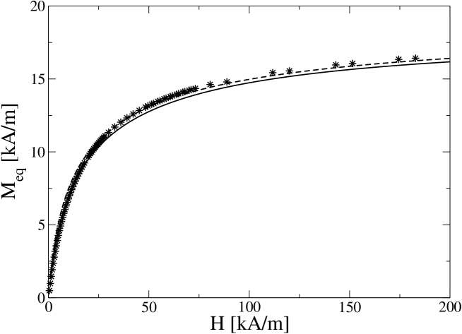
Figure 1: Equilibrium magnetization versus internal magnetic field for the ferrofluid AGP 933 of FerroTec. Symbols denote experimental data, solid line fit with a lognormal distribution, and dashed line fit with a regularization method. See text for further information

Fig. 1 shows the experimentally determined equilibrium magnetization $M_{eq}(H)$ of APG 933 versus internal field $H$ together with fits that were obtained with a lognormal distribution EmMuKrMeNaMuWiLuHeKn01 and with the regularization method EmMaWaKiLeLu06 . The saturation magnetization of the ferrofluid sample was $M_{sat}^{FF}=19108.6$ A/m. From the saturation magnetization the volume concentration of the magnetite particles was found to be $\phi=M_{sat}^{FF}/M_{sat}^{bulk}=4.1$ %, in reasonable agreement with the manufacturer’s specifications. For the initial susceptibility we found the value $\chi_{0}=1.09$.

The magnetic weight distributions $w(d)$ resulting from the two fit methods are shown in Fig. 2.

III Experimental setup

The experimental setup for measuring the magnetization of a rotating cylindrical column of ferrofluid is sketched in Fig. 3. It is described in more detail in EmMaWaKiLeLu06 . The ferrofluid is filled into a cylindrical plexiglass sample holder with inside radius $R=3.2$ mm. This radius is so small that for our rotation frequencies the ferrofluid rotates as a rigid body with a flow field ${\bf u}({\bf r})={\bf\Omega}\times{\bf r}=\Omega r{\bf e}_{\varphi}$. Here $\Omega$ is the externally enforced constant rotation rate of the sample and ${\bf e}_{\varphi}$ is the unit vector in azimuthal direction. A homogeneous and temporally constant magnetic field ${\bf{H}}_{0}=H_{0}{\bf{e}}_{x}$ is applied perpendicular to the cylinder axis ${\bf e}_{z}$. For such a combination of enforced rotation and applied field theoretical models allow for a spatially and temporally constant nonequilibrium magnetization ${\bf M}$ that is pushed out of the directions of ${\bf H}_{0}$ and ${\bf H}$ by the flow.

According to the Maxwell equations the fields ${\bf H}$ and ${\bf M}$ within the ferrofluid are related to each other via

$${\bf H}={\bf H}_{0}-\frac{1}{2}{\bf M}$$ (2)

for our long cylindrical sample and in particular $H_{y}=-M_{y}/2$ as indicated schematically in Fig. 3. In addition they demand that the magnetic field outside the ferrofluid cylinder

$${\bf H}^{out}={\bf H}_{0}+\frac{1}{2}\frac{R^{2}}{r^{2}}\left(2\frac{{\bf r}}{r}\frac{{\bf M}\cdot{\bf r}}{r}-{\bf M}\right)$$ (3)

is a superposition of the applied field ${\bf H}_{0}$ and the dipolar contribution from ${\bf M}$. This result yields a relation between the perpendicular component of the magnetization $M_{y}$ resp. of the internal field $H_{y}=-M_{y}/2$ and the field $H_{y}^{sensor}$ measured by the Hall–sensor outside the sample as indicated in Fig. 3. Considering the finite size of the Hall–sensor, $H_{y}^{sensor}$ is given by

$$H_{y}^{sensor}=\frac{1}{2a}\int_{-a}^{a}H_{y}^{out}dx=-\frac{R^{2}}{a^{2}+b^{2}}H_{y}\,.$$ (4)

In our experimental setup $b=4.75$ mm, $R=3.2$ mm, and $a=2$ mm; here $a$ denotes the horizontal extension of the Hall sensor. So, $H_{y}^{\text{sensor}}=-0.386\,H_{y}$ where $H_{y}=-M_{y}/2$ is the $y$-component of the internal magnetic field in the ferrofluid.

IV Magnetization dynamics of a poly-disperse model

Comparisons with experimental results showed EmMaWaKiLeLu06 that theoretical predictions LeLu06b based on models Sh72 ; FeKr99 ; Fe00 ; Sh01a ; MuLi01 with a single relaxation time overestimate the magnitude of $H_{y}^{sensor}$. One reason is that particles with different sizes and different rotational dynamics of their magnetic moments contribute differently to the non-equilibrium, flow-induced component $M_{y}$ of the magnetization and that in particular only the magnetic moments of the larger particles with effective Brownian relaxation dynamics may be rotated by the flow out of the direction of the magnetic field.

Therefore, we consider here as a next step poly-disperse models with single-particle Brownian and Néel relaxation dynamics for the different particle sizes. Such models have been used LeLu06a to determine within a linear response analysis the effect of polydispersity on the dynamics of a torsional ferrofluid pendulum that was periodically forced close to resonance to undergo small amplitude oscillations in a rigid body flow EmMuWaKnLu00 ; EmMuLuKn00 .

We ignore the influence of any dipolar magnetic interaction and of any flow induced interaction on the (rotation) dynamics of the particles. Thereby collective, collision dominated long-range and long-time hydrodynamic relaxation dynamics of the ensemble of magnetic moments are discarded since only the individual relaxation of each magnetic moment is considered — albeit in the collectively generated internal magnetic field ${\bf H}$.

For numerical reasons we use a discrete partition of the particle size distribution. Then, without interaction, the magnetization of the resulting mixture of mono-disperse ideal paramagnetic gases is given by ${\bf M}=\sum{\bf M}_{j}$, where ${\bf M}_{j}$ denotes the magnetization of the particles with diameter $d_{j}$. We assume that each magnetic moment and with it each ${\bf M}_{j}$ obeys a simple Debye relaxation dynamics that drives them in the absence of flow towards their respective equilibrium value ${\bf M}_{j}^{eq}({\bf H})$. Then, in the stationary situation resulting from the rigid body rotation with constant ${\bf\Omega}$ the Debye relaxation equation for each sub magnetization is given by

$${\bf\Omega}\times{\bf M}_{j}=\frac{1}{\tau_{j}}[{\bf M}_{j}-{\bf M}_{j}^{eq}({\bf H})]\,.$$ (5)

In the absence of interactions the equilibrium magnetization of each species is determined by a Langevin function

$${\bf M}_{j}^{eq}({\bf H})=\chi_{j}(H){\bf H}=w_{j}{\cal L}\left(\frac{\mu_{0}\pi M_{sat}^{bulk}}{6k_{B}T}d_{j}^{3}H\right)\,\frac{{\bf H}}{H}\,.$$ (6)

Here $M_{sat}^{bulk}$ is the bulk-saturation magnetization of the magnetic material. For the magnetic weight $w_{j}(d_{j})$ of species $j$ we take the experimentally determined values in the representation (1).

We should like to draw the attention of the reader to the fact that the magnetization equations (5) for the different particle sizes are coupled via the internal field ${\bf H}$: according to Maxwell’s equations ${\bf H}={\bf H}_{0}-\frac{1}{2}{\bf M}$ is given in terms of the total ${\bf M}=\sum{\bf M}_{j}$.

In the relaxation rate $1/\tau_{j}$ we take into account Brownian and Néel relaxation processes by adding their rates with equal weight

$$\frac{1}{\tau_{j}}=\frac{1}{\tau_{B}^{j}}+\frac{1}{\tau_{N}^{j}}\,.$$ (7)

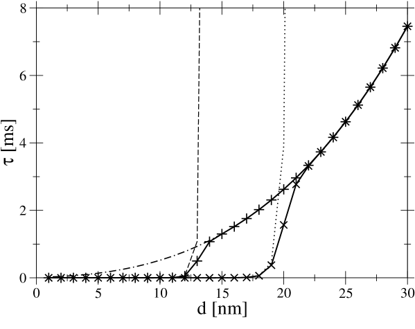
Figure 4: Relaxation times as a function of particle diameter $d$: Brownian (dot-dashed line), Néel (dotted line for $K=15kJ/m^{3}$, dashed line for $K=50kJ/m^{3}$), and the combination (7) (solid line with crosses for $K=15kJ/m^{3}$, solid line with plusses for $K=50kJ/m^{3}$).

The relaxation times depend on the particle size according to $\tau_{B}^{j}=\frac{\pi\eta}{2k_{B}T}(d_{j}+2s)^{3}$ and $\tau_{N}^{j}=f_{0}^{-1}\exp\left(\frac{\pi Kd_{j}^{3}}{6k_{B}T}\right)$. Her $\eta$ is the viscosity, $s$ the thickness of the nonmagnetic particle layer, and $K$ the anisotropy constant. The combined relaxation rate (7) is dominated by the faster of the two processes. Thus, large particles relax in a Brownian manner with relaxation times of about some $10^{-3}s$, while small particles have the much smaller Néel relaxation times. The boundary between Néel and Brownian dominated relaxation as a function of particle size $d$ depends sensitively on the anisotropy constant $K$. This is documented in Fig. 4 for the two values $K=15kJ/m^{3}$ and $K=50kJ/m^{3}$. For these specific examples the boundaries between Néel and Brownian dominated relaxation lie at about $d\simeq 20nm$ and $d\simeq 13nm$, respectively.

V Comparison with experiments

For the numerical calculations we take typical values for the ferrofluid APG 933 of FerroTec that is used among others in the experiments described in EmMaWaKiLeLu06 : $M_{sat}^{bulk}=456kA/m$, $\eta=0.5Pa\,s$, $s=2nm$, and $f_{0}=10^{9}Hz$. Typical values of $K$ lie between $10kJ/m^{3}$ and $50kJ/m^{3}$ FaPrCh99 ; Fa94 . We furthermore use as input the experimental equilibrium magnetization $M_{eq}(H)$ of APG 933 shown in Fig. 1 and the magnetic weights of Fig. 2 obtained with fits to a log-normal distribution or with a regularization method EmMaWaKiLeLu06 .

From the previous work LeLu06b ; EmMaWaKiLeLu06 we know that single-relaxation time (mono-disperse) models predict the maximum of $M_{y}$ resp. of $H_{y}^{sensor}$ to be located roughly at $\Omega\tau\sim 1$. Furthermore, in the experiments EmMaWaKiLeLu06 done with poly-disperse ferrofluids for frequencies up to $\Omega\simeq 3000rad/s$ mainly the large particles contribute to $M_{y}$ resp. to $H_{y}^{sensor}$ since their magnetic moments are effectively frozen in the particle’s crystal lattice. Only these magnetic moments can be pushed out of the direction of the magnetic field by the combined action of thermally induced rotary Brownian motion and deterministic macroscopic flow in the rotating cylinder. Smaller particles can keep their moment aligned with the magnetic field by the Néel process when these particles undergo rotational motion. Finally, the particle diameter that separates Néel behavior from Brownian behavior in the size distribution and that thereby determines how many particles contribute to $M_{y}$ resp. to the experimental signal $H_{y}^{sensor}$ depends sensitively on the anisotropy constant $K$: The smaller $K$, the smaller is the number of Brownian particles according to Fig. 4, and the smaller is $M_{y}$ resp. $H_{y}^{sensor}$.

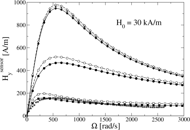
Figure 5: $H_{y}^{sensor}$ as function of $\Omega$ for $H_{0}=30kA/m$. The three uppermost curves refer to single-time relaxation approximations, each with $\tau=2ms$: monodisperse Debye model (dotted line with crosses), polydisperse models with common $\tau_{j}=\tau$ and magnetic weights $w_{j}$ obtained with a lognormal distribution (full line with full diamonds) and with a regularization method (dashed line with open diamonds). Curves with circles and squares refer to truly polydisperse models [ eqs. (5 - 7)] with $K=50kJ/m^{3}$ (circles) and $K=15kJ/m^{3}$ (squares). Full lines with full symbols were obtained with a lognormal distribution. Dashed lines with open symbols refer to a distribution resulting from the regularization method. In all models the equilibrium magnetization $M_{eq}(H)$ was taken to be the experimental one.

The above sketched physical picture is corroborated by Fig. 5. There we compare the experimentally obtained $H_{y}^{sensor}(\Omega)$ (stars) as a function of $\Omega$ for a representative externally applied field $H_{0}=30kA/m$ with various model variants that take into account the polydispersity to different degrees. This is done for two different anisotropy constants, namely, $K=15kJ/m^{3}$ and $K=50kJ/m^{3}$ as representative examples. However, the three uppermost curves refer to single time relaxation approximations, each with $\tau=2ms$ EmMaWaKiLeLu06 : the dotted line with crosses is the result of a strictly monodisperse Debye model while the lines with diamonds refer to polydisperse models, however, with common $\tau_{j}=\tau=2ms$ taken in Eq. (5) but different magnetic weights $w_{j}$ obtained either from a lognormal distribution (full line with full diamonds) or from the regularization method (dashed line with open diamonds). The equilibrium magnetization $M_{eq}(H)$ was taken to be the experimental one, the distributions were obtained from this experimental $M_{eq}(H)$ by the lognormal ansatz resp. the regularization method. This, first of all, shows that models with only one relaxation time show roughly the same behavior of $M_{y}(\Omega)$ irrespective of whether the particle size and magnetic moment distributions are polydisperse or not.

The set of curves with circles and squares in Fig. 5 refer to truly polydisperse models, eqs. (5 - 7), but different anisotropy constants of the magnetic material [$K=50kJ/m^{3}$ (circles), $K=15kJ/m^{3}$ (squares)]. Again, full lines with full symbols were obtained with a lognormal distribution while dashed lines with open symbols refer to a distribution resulting from the regularization method. Here, one sees that these two distributions with their magnetic weights displayed in Fig. 2 yield very similar results which might not be surprising in view of the fact that both seem to reproduce $M_{eq}(H)$ adequately.

The largest and most important difference between the curves with diamonds (i.e., the single-time models) and the curves with circles and squares (i.e., the genuine polydisperse models) come from the difference in the anisotropy constants of the magnetic material that governs how many particles contribute efficiently as Brownian ones to the transverse magnetization $M_{y}$ resp. to $H_{y}^{sensor}$: for smaller $K$ the magnetic moments of fewer particles being Brownian ones may be rotated out of the direction of the magnetic field by the flow in the cylinder.

The curves for $K=15kJ/m^{3}$ yield roughly the same maximal size $H_{y}^{sensor}$ as the experiments — they could be fine-tuned even further. But then the location, $\Omega^{max}(H_{0})$, of the maxima for different $H_{0}$ is still off from the experimental ones as shown in Fig. 6(a) and 7(b). However, the agreement between the predictions of the polydisperse models of eqs. (5 - 7) and the experiments concerning the location $\Omega^{max}(H_{0})$ can be improved by allowing the relaxation rates $\tau_{j}$ of the differently sized particles to depend also on the internal field $H$. To demonstate this, we use for simplicity the form EmMaWaKiLeLu06

$$\tau_{j}^{\gamma}(H)=\tau_{j}\,\frac{2{\cal L}(\gamma H)}{\gamma H-{\cal L}(\gamma H)}$$ (8)

with one additional fit parameter $\gamma$. Values of about $\gamma\sim 10^{-4}m/A$ yield maximum locations $\Omega^{max}(H_{0})$ that agree well with the experiments as can be seen in Fig. 6(b) and Fig. 7(b). This generalization of the model (5 - 7) leaves the peak value $H_{y}^{sensor}(\Omega^{max})$ almost unchanged, cf, Fig. 7(a).

However, also this augmented polydispersive model reproduces with fixed values of $K$ and $\gamma$ the experimental data only in a small range of $\Omega$ and $H_{0}$, cf, Fig. 6 and Fig. 7.

VI Conclusion

We have compared the predictions of polydisperse models of the magnetization dynamics of ferrofluids with recent experiments measuring the transverse magnetization component $M_{y}$ of a rotating ferrofluid cylinder. The models use mixtures of mono-disperse ideal paramagnetic gases of differently sized particles. The magnetization dynamics of the models take into account the rigid body rotation of the fluid combined with a simple Debye relaxation of the magnetic moments of each particle with size dependent Brownian and Néel magnetic relaxation times. Thus, in the absence of flow, each magnetic moment and with it each sub-magnetization would be driven independently of the others towards its respective mean equilibrium value that, however, depends on the internal magnetic field ${\bf H}$ being collectively generated by all magnetic moments.

The comparison suggests that mainly the large particles contribute to $M_{y}$ since their magnetic moments are effectively frozen in the particle’s crystal lattice. Only these magnetic moments can be pushed effectively out of the direction of the magnetic field by the combined action of thermally induced rotary Brownian motion and deterministic macroscopic flow in the rotating cylinder. Smaller particles can keep their moment aligned with the magnetic field by the Néel process when these particles undergo rotational motion.

Finally, the particle diameter that separates Néel behavior from Brownian behavior in the size distribution and that thereby determines how many particles contribute to $M_{y}$ resp. to the experimental signal $H_{y}^{sensor}$ depends quite sensitively on the anisotropy constant $K$ of the magnetic material. $K$ determines how many magnetic moments are ”frozen” or ”blocked” in particles and thus can be rotated by the rigid body flow: The smaller $K$, the smaller is the number of Brownian particles with frozen moments, and the smaller is the resulting $M_{y}$. Or, vice versa, a large transverse magnetization can be expected in ferrofluids with large anisotropy constants.

An analysis of the rotation rates $\Omega^{max}(H_{0})$ for which $M_{y}$ is largest indicates that the agreement between experiments and model predictions can be improved by allowing the relaxation rates of the differently sized particles to depend also on the magnetic field $H$.

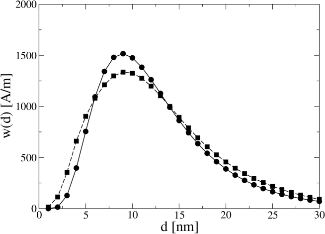
Figure 2: Magnetic weights of the 30 here considered particle sizes ($d_{1}=1nm$ to $d_{30}=30nm$) obtained from measurements of $M_{eq}(H)$ in Fig.1 by using a lognormal distribution (solid line, circles) and by using a regularization method (dashed line, squares).

Figure 3: Schematic plot of the system. The cylindrical sample holder with inner radius $R$ rotates with angular velocity $\boldsymbol{\Omega}$ in the applied static magnetic field ${\bf{H}}_{0}$ perpendicular to $\boldsymbol{\Omega}$. The magnetization $M_{y}$ is measured with a Hall sensor. ${\bf M}$ and ${\bf H}$ denote the magnetization and internal magnetic field of the ferrofluid. Both are constant in space and time.

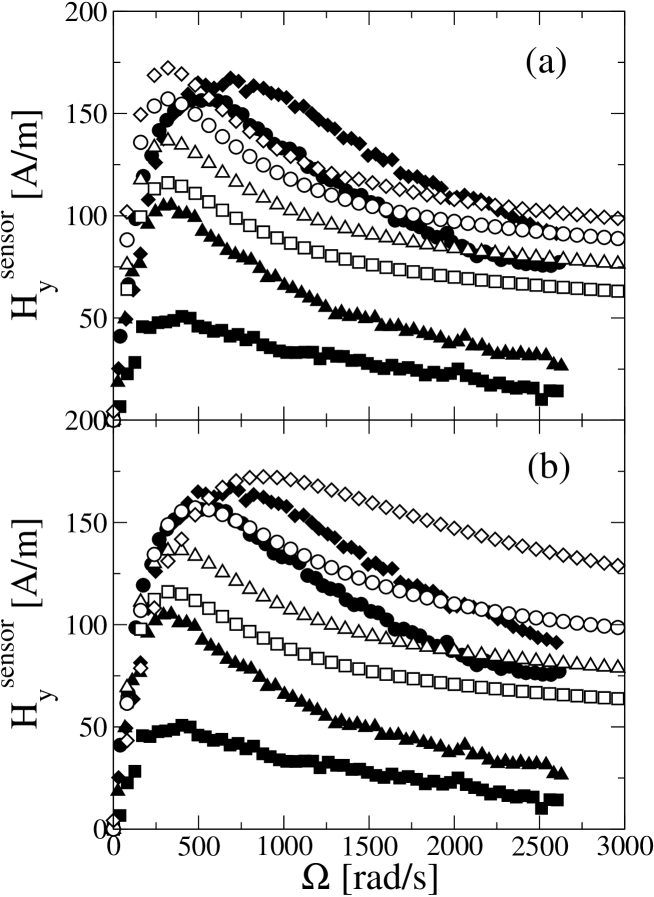
Figure 6: $H_{y}^{sensor}$ as function of $\Omega$ for $H_{0}=8.6kA/m$ (squares), $15kA/m$ (triangles), $30kA/m$ (circles), and $60kA/m$ (diamonds). Full symbols denote experimental data. Open symbols refer to the polydisperse model [eqs. (5 - 7)] with lognormal distribution and $K=15kJ/m^{3}$: in (a) the relaxation times $\tau_{j}$ are independent of $H$, in (b) they are replaced by $\tau_{j}^{\gamma}(H)$ (8) with $\gamma=10^{-4}m/A$.

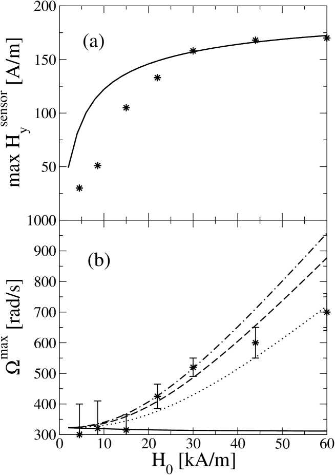
Figure 7: Maximum magnitude $maxH_{y}^{sensor}=H_{y}^{sensor}(\Omega^{max})$ (a) and location of the maximum $\Omega^{max}$ (b) as functions of the external field $H_{0}$. Stars show experimental data. Lines refer to the results of polydisperse models with a lognormal distribution and $K=15kJ/m^{3}$: $H$-independent relaxation times (solid); $H$–dependencies with $\gamma=0.8\cdot 10^{-4}m/A$ (dotted), $\gamma=10^{-4}m/A$ (dashed), and $\gamma=1.1\cdot 10^{-4}m/A$ (dot-dashed). In (a) the differences between the lines are too small to be seen.

- (1) R. E. Rosensweig, Ferrohydrodynamics (Cambridge University Press, Cambridge, 1985).
- (2) E. Blums, A. Cebers, and M. M. Maiorov, Magnetic Fluids (Walter de Gruyter, Berlin, 1997).
- (3) S. Odenbach, Magnetoviscous Effects in Ferrofluids, Vol. m71 of Lecture Notes in Physics (Springer, Berlin, 2002).
- (4) Ferrofluids - Magnetically controllable Fluids and their Applications, Vol. 594 of Lecture Notes in Physics, edited by S. Odenbach (Springer, Berlin, 2002).
- (5) J. P. McTague, J. Chem. Phys. 51, 133 (1969).
- (6) J. P. Embs, S. May, C. Wagner, A. V. Kityk, A. Leschhorn, and M. Lücke, Phys. Rev. E 73, 036302 (2006).
- (7) A. Leschhorn and M. Lücke, Z. Phys. Chem. 220, 219 (2006).
- (8) M. I. Shliomis, Sov. Phys. JETP 34, 1291 (1972).
- (9) B. U. Felderhof and H. J. Kroh, J. Chem. Phys. 110, 7403(1999).
- (10) B. U. Felderhof, Phys. Rev. E 62, 3848 (2000).
- (11) M. I. Shliomis, Phys. Rev. E 64, 060501 (2001).
- (12) H. W. Müller and M. Liu, Phys. Rev. E 64, 061405 (2001).
- (13) J. Embs, H. W. Müller, C. E. Krill, F. Meyer, H. Natter, H. Müller, S. Wiegand, M. Lücke, R. Hempelmann, and K. Knorr, Magnetohydrodynamics 37, 222 (2001).
- (14) T. Weser and K. Stierstadt, Z. Phys. B Cond. Mat. 59, 253 (1985).
- (15) A. Leschhorn and M. Lücke, Z. Phys. Chem. 220, 89 (2006).
- (16) J. Embs, H. W. Müller, C. Wagner, K. Knorr, M. Lücke, Phys. Rev. E 61, R2196 (2000).
- (17) J. Embs, H. W. Müller, M. Lücke, and K. Knorr, Magnetohydrodynamics 36, 387 (2000).
- (18) P. C. Fannin, P. A. Preov, and S. W. Charles, J. Phys. D 32,1583 (1999).
- (19) P. C. Fannin, J. Magn. Magn. Mater. 136, 49 (1994).