Frequency analysis of tick quotes on the foreign exchange market
and agent-based modeling: A spectral distance approach

Abstract

High-frequency financial data of the foreign exchange market (EUR/CHF, EUR/GBP, EUR/JPY, EUR/NOK, EUR/SEK, EUR/USD, NZD/USD, USD/CAD, USD/CHF, USD/JPY, USD/NOK, and USD/SEK) are analyzed by utilizing the Kullback-Leibler divergence between two normalized spectrograms of the tick frequency and the generalized Jensen-Shannon divergence among them. The temporal structure variations of the similarity between currency pairs is detected and characterized. A simple agent-based model in which $N$ market participants exchange $M$ currency pairs is proposed. The equation for the tick frequency is approximately derived theoretically. Based on the analysis of this model, the spectral distance of the tick frequency is associated with the similarity of the behavior (perception and decision) of the market participants in exchanging these currency pairs.

PACS numbers: 89.65.Gh,02.50.-r,02.70.Hm

1 Introduction

The recent accumulation of high-frequency financial data due to the development and spread of information and communications technology has sparked interest in financial markets [1, 2, 3, 4, 5, 6, 7, 8, 9, 10]. Many researchers expect new findings and insights into the worlds of both finance and physics. Since the financial markets are complex systems that consist of several agents that interact with one another, an enormous amount of data must be treated in order to describe and understand them at the microscopic level. Therefore, it is important to find adequate variables or relevant quantities to describe their properties [11]. Since a macroscopic description allows information with global properties to be compressed, if the adequate macroscopic quantities can be determined, then relationships can be established among various macroscopic quantities and a deeper understanding of the system can be obtained.

On the other hand, agent-based models as complex systems are attracting significant interest across a broad range of disciplines. Several agent-based models have been proposed to explain the behavior of financial markets during the last decade [12, 13, 14, 15, 16, 17, 18]. Agent-based models are expected to provide an alternative to phenomenological models that mimic market price fluctuations. Specifically, it seems to be worth considering the explanation capability of the agent-based models for causality from a microscopic point of view.

In a previous study, the tick frequency, which is defined as the number of tick quotations per unit time, was reported to exhibit periodic motions due to the collective behavior of the market participants [19, 20]. As a result, the tick frequency appears to be an important representative quantity in the financial market. Moreover, it has been reported that it is possible to detect the dynamic structure of the foreign exchange market by using the spectral distance defined by the Kullback-Leibler divergence [21]. The spectral distance of the tick frequency is one possibility for macroscopically describing the relationship among market participants in the financial market.

In the present study, the meaning of the spectral distance of the tick frequency is discussed, starting from the microscopic description with the agent-based model of a financial market. First, definitions and the results of the spectral distance of the tick frequency are presented. Next, a model that consists of $N$ market participants who choose their action among three kinds of investment attitudes in order to exchange $M$ currency pairs is considered. In this model, the heterogeneous agents perceive information in the environment, which is separated into exogenous factors (news about events) and endogenous factors (news about market fluctuations), and decide their actions based on these factors. There are two thresholds by which to select their actions among three kinds of investment attitudes (buying, selling, and waiting). Analysis of this model indicates that the spectral distance of the tick frequency is equivalent to the difference among behavioral parameters of market participants who exchange these currency pairs.

This remainder of this paper is organized as follows. In Section 2, the tick frequencies of 12 currency pairs in the foreign exchange market are analyzed with the spectral distance measured by the Kullback-Leibler divergence and the Jensen-Shannon divergence of the normalized power spectra. In Section 3, an agent-based model in which $N$ market participants deal with $M$ currency pairs is proposed. In Section 4, based on the agent-based model, the equation for the tick frequency is approximately derived, and the relationship between the spectral distance of the tick frequency and the behavioral parameters of market participants is discussed. Section 5 is devoted to concluding remarks.

2 Frequency analysis

2.1 Data

The foreign currency market data of United States Dollar (USD), Euro (EUR), Switzerland Francs (CHF), Great Britain Pounds (GBP), Norwegian Krone (NOK), Swedish Krona (SEK), Canadian Dollars (CAD), New Zealand Dollars (NZD), and Japanese Yen (JPY), as provided by CQG Inc., were investigated [22]. The data include two quote rates, namely, the bid rate and the ask rate, with a resolution of one minute. The bid and ask rates are the prices at which bank traders are willing to buy and sell a unit of currency. All traders in the foreign exchange market have a rule to quotes both rates at the same time (two-way quotation). Generally, the ask rate is higher than the bid rate, and the difference between the bid rate and the ask rate is called the bid-ask spread.

The data investigated in this article are from two databases. The first includes 12 currency pairs, EUR/CHF, EUR/GBP, EUR/JPY, EUR/NOK, EUR/SEK, EUR/USD, NZD/USD, USD/CAD, USD/CHF, USD/JPY, USD/NOK, and USD/SEK, during the period from the 1st to the 29th of September 2000. The other includes three currency pairs, EUR/USD, EUR/JPY, and USD/JPY, during the period from the 4th of January 1999 to the 31st of December 2004. The data start at 17:00 (CST) on Sunday, and finish at 16:59 (CST) on Friday. The foreign exchange market is open for 24 hours on weekdays. On Saturdays and Sundays, there are no ticks on the data set because most banks are closed.

2.2 Methods

The tick frequency is defined by counting the number of times that bank traders quote the bid and ask rates per unit time. According to this definition a currency pair having a high (low) quote frequency indicates activity (inactivity). Since bank traders usually quote both bid and ask rates at the same time, it is sufficient to count only the bid or the ask quotation. Here, the tick frequency is defined as the number of ask quotes per unit time,

$$A(k)=\frac{1}{\Delta t}C(k\Delta t;(k+1)\Delta t),\quad(k=0,1,\ldots)$$ (1)

where $C(t_{1};t_{2})$ is the number of the ask quotes from $t_{1}$ to $t_{2}$, and $\Delta t$ denotes the sampling period, and $\Delta t=1$ minutes throughout this analysis.

The spectrogram is estimated with a discrete Fourier transform for a time series multiplied by the Hanning window. Let $A(k)\quad(k=0,1,2,\ldots)$ be the time series of tick frequencies. The spectrogram with the Hanning window represented as

$$w(k)=\frac{1}{2}\Bigl{(}1-\cos(\frac{2\pi k}{L-1})\Bigr{)},$$ (2)

is defined as

$$P(n,T) = \Bigl{|}\sum_{k=0}^{L-1}w(k)A(k+T)e^{-2\pi\mbox{i}k\frac{n}{L}}\Bigr{|}^{2},$$ (3)

where $T$ denotes the representative time to localize the data by the window function having the range of $L\Delta t$. Since the Nyquist critical frequency is given by $f_{c}=1/(2\Delta t)=0.5$ [1/min], the behavior of the market participants can be detected with a resolution of 2 [min].

For the purpose of quantifying the similarity between the tick frequencies, the Kullback-Leibler (KL) divergence method is applied between normalized spectrograms of the tick frequency [19]. The KL is defined as a functional of two normalized positive functions [23]. In order to apply the KL method to the spectrogram, the normalized spectrogram is introduce as follows:

$$p(n,T)=\frac{P(n,T)}{\sum_{n=1}^{L-1}P(n,T)}.$$ (4)

The KL between the spectrograms without the direct current component for the $i$-th currency pair, $p_{i}(n,T)$, and that for the $j$-th currency pair, $p_{j}(n,T)$, is defined as

$$K_{ij}(T)=\sum_{n=1}^{L-1}p_{i}(n,T)\log\frac{p_{i}(n,T)}{p_{j}(n,T)}.$$ (5)

Based on its definition, the KL is always non-negative,

$$K_{ij}(T)\geq 0,$$ (6)

with $K_{ij}(T)=0$ if and only if $p_{i}(n,T)=p_{j}(n,T)$. Note that $K_{ij}(T)$ is an asymmetric dissimilarity matrix, which is satisfied by

$$K_{ij}(T)\neq K_{ji}(T),K_{ii}(T)=0.$$ (7)

Generally, the asymmetric matrix is separated into a symmetric matrix and an asymmetric matrix,

$$K_{ij}(T)=J_{ij}(T)+I_{ij}(T),$$ (8)

where $J_{ij}(T)=(K_{ij}(T)+K_{ji}(T))/2$, $I_{ij}(T)=(K_{ij}(T)-K_{ji}(T))/2$. Specifically, $J_{ij}(T)$ is called the symmetrical Kullback-Leibler distance (SKL) and is defined as follows:

$$J_{ij}(T)=\frac{1}{2}\sum_{n=1}^{L-1}(p_{i}(n,T)-p_{j}(n,T))\log\frac{p_{i}(n,T)}{p_{j}(n,T)},$$ (9)

where $J_{ij}(T)=J_{ji}(T)$, $J_{ii}(T)=0$, and $J_{ij}(T)=0$ if and only if $p_{i}(n,T)=p_{j}(n,T)$.

As an alternative symmetric divergence, the Jensen-Shannon divergence (JS) [24] is defined as follows:

$$JS_{ij}^{\pi}(T)=H(\pi_{i}p_{i}+\pi_{j}p_{j},T)-\pi_{i}H(p_{i},T)-\pi_{j}H(p_{j},T),$$ (10)

where $\pi_{i},\pi_{j}>0$, $\pi_{i}+\pi_{j}=1$ are the a priori probability for $p_{i}$ and $p_{j}$, and $H(p,T)$ is the Shannon entropy, which is defined as $H(p,T)=-\sum_{n=1}^{L-1}p(n,T)\log p(n,T)$. This divergence possesses symmetric and non-negative features: $JS_{ij}^{\pi}(T)=JS_{ji}^{\pi}(T)$, $JS_{ij}^{\pi}(T)\geq 0$, and $JS_{ij}^{\pi}(T)=0$ if and only if $p_{i}(n,T)=p_{j}(n,T)$. Moreover, it is possible to calculate the total similarity of the market using the generalized Jensen-Shannon divergence (GJS),

$$JS^{\pi}(p_{1},p_{2},\ldots,p_{M})=H\Bigl{(}\sum_{i=1}^{M}\pi_{i}p_{i}\Bigr{)}-\sum_{i=1}^{M}\pi_{i}H(p_{i}).$$ (11)

The GJS is non-negative, i.e., $JS^{\pi}(p_{1},p_{2},\ldots,p_{M})\geq 0$ and $JS^{\pi}(p_{1},p_{2},\ldots,p_{M})=0$, if and only if $p_{1}(n,T)=p_{2}(n,T)=\cdots=p_{M}(n,T)$.

2.3 Results

Figure 1 shows the SKL among 12 currency pairs for the Asian time zone ($T=$0:00 (UTC+1)), the European time zone ($T=$8:00 (UTC+1)), and the American time zone ($T=$16:00 (UTC+1)) as fully connected networks.

The patterns in Fig. 1 indicate the existence of similar currency pairs and dissimilar currency pairs at each time zone. The similarity and dissimilarity between currency pairs varies temporally. Furthermore, the variations of the network structure are slow. The results obtained using the JS provide are similar to those obtained using the SKL.

As shown in Fig. 2 the GJS among 12 currency pairs under the uniform condition $\pi_{i}=1/12$ varies periodically. This periodic variation is thought to be due to the life cycle of the market participants. Specifically, the GJS becomes low at the time between time zones. Outliers, which look like pulses, occasionally occur, indicating drastic changes in the similarity structure at a specific time.

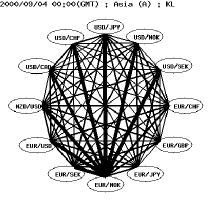
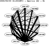
Figure 1: The symmetrical Kullback-Leibler distance among 12 currency pairs for the Asian time zone ($T=$0:00 (UTC+1)) (left), the European time zone ($T=$8:00 (UTC+1)) (center), and the American time zone ($T=$16:00 (GMT)) (right) on the 4th of September 2000 for $N=480$ (8 hours). The thin/thick lines between the $i$-th currency pair and the $j$-th currency pair represent the similarity/dissimilarity between them, $J_{ij}(T)$.

Figure 2: Time series of the generalized Jensen-Shannon divergence among 12 currency pairs with $L=480$ [min] on the 4th of September 2000.

The results of the SKL divergences among the EUR/USD, the USD/JPY, and the EUR/JPY during the period from the 4th of January 1999 to the 31st of December 2004 are shown in Fig. 4. The SKL divergences decrease yearly and have high values around the first day of each year.

The results of the GJS among the EUR/USD, the USD/JPY, and the EUR/JPY during the period from the 4th of January 1999 to the 31st of December 2004 are shown in Fig. 5. The GJS values in 1999 are relatively higher than those after 2001. For the period from the middle of 1999 to the middle of 2000, the GJS values remain high. The GJS values decrease from the middle of 2000 and tend to be less than 0.1. After the middle of 2000 the GJS values remain low. Hence, comparing tick frequency behavior before and after mid 2000, revealed that tick frequencies in the foreign exchange market after mid 2000 became increasingly similar to those in the first half of that year. The similarity of the recent market appears to be the similarity in the behavior of market participants all over the world as a result of the development of information and communication technology.

Table 1: Daily averages in April 2001, in millions of US dollars and percentages.

time zone	USD	EUR	JPY
Asian time zone	373,179 (25.3%)	74,745 (12.2%)	160,384 (43.4%)
European time zone	806,997 (54.8%)	430,156 (70.3%)	137,731 (37.3%)
American time zone	292,563 (19.9%)	106,909 (17.5%)	71,448 (19.3%)
Total	1,472,739 (100%)	611,810 (100%)	369,563 (100%)

According to the Triennial Central Bank Survey 2001 [25], the turnover by currency pairs in cross-border double-counting is reported to be 30% for USD/EUR, 20% for USD/JPY, and 3% for EUR/JPY. As shown in Table 1 by the share of currencies for various time zones, the USD and the EUR are the most actively traded in the European time zone and the JPY is actively traded in both the Asian time zone and the European time zone. Table 1 indicates that European market participants are active. Given that market participants in the European market primarily trade with the EUR as an axis, it is predicted that the EUR/USD and the EUR/JPY between Asia and Europe and Europe and America will behave similarly in time, and that the dissimilarities among the EUR/USD, USD/JPY, and EUR/JPY are likely to arise when the European market opens.

Both characteristics are found in the temporal development of the SKL, as shown in Fig. 3. The property whereby the spectral distance is small at the time between the Asian time zone and the European time zone, and between the European time zone and American time zone, is also found in the GJS among 12 currency pairs (Fig. 2). It is thought that the market participants in each time zone tend to exchange currencies with the market participants in other time zones.

Figure 3: The symmetric Kullback-Leibler divergence of spectrograms between the EUR/JPY and the EUR/USD (solid line), between the EUR/USD and the USD/JPY (long-dashed line), and between the EUR/JPY and the EUR/USD (short-dashed line) on the 4th of September 2000.

(a) (b) (c)

Figure 4: The Kullback-Leibler divergence of spectrograms between the EUR/USD and the EUR/JPY (a), between the EUR/USD and the USD/JPY (b), and between the EUR/USD and the EUR/JPY (c) for the period between the 4th of January 1999 and the 31st of December 2004.

Figure 5: The generalized Jensen-Shannon divergence of spectrograms among the EUR/USD, USD/JPY, and EUR/JPY for the period between the 4th of January 1999 and the 31st of December 2004.

3 Agent-based model

Consider $N$ market participants who deal with $M$ currency pairs. The $i$-th market participant perceives information $x_{i}(t)$ from the environment. Based on this information the participant determines his/her own investment attitude. Let $y_{ij}(t)$ denote the investment attitude of the $i$-th market participant for the $j$-th currency pair. The market participants are able to select his/her action from among three investment attitudes (buying, selling, and waiting).

According to the Virginia Satir seven step model from perception to action, which is one of psychological models of human [26], an agent-based model of the foreign exchange market is considered. In the Virginia Satir model, the process from perception to action is separated into seven main steps: perception of information, interpretation, feeling, feeling about the feeling, defense, rule for acting, and action.

For simplicity, the $i$-th market participant perceives information $x_{i}(t)$, which is evaluated as a scalar value. This information builds momentum for the market participant to decides his/her investment attitude. The market participant interprets the information and determines his/her attitude on the basis of the interpretation. Since the possibility of interpretation is very high and is dependent on time and market participants, the uncertainty for the $i$-th agent to interpret the information $x_{i}(t)$ a time $t$ is uniquely modeled by a random variable $\xi_{i}(t)$. It is assumed that the result of the interpretation $x_{i}(t)+\xi_{i}(t)$ drives feeling, determining his/her investment attitude. Furthermore, the feeling about the feeling examines the validity of the feeling and drives his/her actions. In order to model the feeling about the feeling, a multiplicative factor $a_{ij}(t)$, which represents the feeling about the feeling of the $i$-th market participant for the $j$-th currency pair, is introduced. If $a_{ij}(t)$ is positive, then the feeling about the feeling supports the feeling. If $a_{ij}(t)$ is negative, then the feeling about the feeling refutes the feeling. The absolute value of $a_{ij}(t)$ represents the intensity of the feeling about the feeling. Since the determination depends on both the feeling and the feeling about the feeling, the investment attitude is assumed to be determined from the value $a_{ij}(t)(x_{i}(t)+\xi_{i}(t))$. If it is large, then the market participant tends to make a buy decision. Contrarily, if it is small then the market participant tends to make a sell decision. For simplicity, it is assumed that a trading volume can be ignored.

The action is determined on the basis of the feeling about the feeling of the market participant. Since the decision and action have strong nonlinearity, the action is determined with Granovetter type threshold dynamics [27]. In order to separate three actions, at least two thresholds are needed. Defining the threshold for the $i$-th market participant to decide to buy the $j$-th currency pair as $\theta_{ij}^{B}(t)$ and to sell it as $\theta_{ij}^{S}(t)$ ($\theta_{ij}^{B}(t)>\theta_{ij}^{S}(t)$), three investment attitudes (buying: 1, selling: -1, and waiting: 0) are determined by

$$y_{ij}(t)=\left\{\begin{array}[]{ll}1&(a_{ij}(t)(x_{i}(t)+\xi_{i}(t))\geq\theta_{ij}^{B}(t))\\ 0&(\theta_{ij}^{B}(t)<a_{ij}(t)(x_{i}(t)+\xi_{i}(t))<\theta_{ij}^{S}(t))\\ -1&(a_{ij}(t)(x_{i}(t)+\xi_{i}(t))\leq\theta_{ij}^{S}(t))\end{array}\right.$$ (12)

Furthermore, it is assumed that the information is described as the endogenous factor, the moving average of the log return over $T_{ij}(t)$, plus the exogenous factor, $s_{i}(t)$:

$$x_{i}(t)=\sum_{k=1}^{M}C_{ik}(|\theta_{ik}^{S}(t)|,|\theta_{ik}^{B}(t)|)\frac{1}{T_{ik}(t)}\sum_{\tau=1}^{T_{ij}(t)}R_{j}(t-\tau\Delta t)+s_{i}(t),$$ (13)

where $C_{ij}(|\theta_{ij}^{S}(t)|,|\theta_{ij}^{B}(t)|)$ represent the focal points of the $i$-th market participant for the $j$-th currency pair. It seems reasonable to assume that $C_{ij}(x,y)$ is a monotonically decreasing function of $x$ and $y$.

The excess demand for the $j$-th currency pair, $N^{-1}\sum_{i=1}^{N}y_{ij}(t)$, drives the market price of the $j$-th currency pair [28]. To guarantee positive market prices, the following log return is chosen:

$$R_{j}(t)=\log S_{j}(t+\Delta t)-\log S_{j}(t),$$ (14)

and define the log returns as the excess demand,

$$R_{j}(t)=\gamma N^{-1}\sum_{i=1}^{N}y_{ij}(t),$$ (15)

where $\gamma$ is a positive constant to show the response of the return to the excess demand. Furthermore, the tick frequency for the $j$-th currency pair is defined as

$$A_{j}(t)=\frac{1}{\Delta t}\sum_{i=1}^{N}|y_{ij}(t)|.$$ (16)

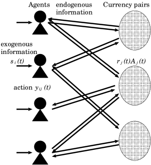
Figure 6: A conceptual illustration of the agent model. $N$ market participants (agents) attend the market in order to exchange $M$ currency pairs.

4 Discussion

Since the market participants have a limitation due to finite time and capacity to perceive the information and determine the investment attitude, it is reasonable to assume that $T_{ij}(t)$ is finite and constant, i.e., $T_{ij}(t)=T_{ij}$. Furthermore, for simplicity, it is assumed that $\xi_{i}(t)$ is sampled from the independent Gaussian distribution,

$$p_{\xi}(\xi_{i})=\frac{1}{\sqrt{2\pi}\sigma}\exp\Bigl{(}-\frac{\xi_{i}^{2}}{2\sigma^{2}}\Bigr{)},$$ (17)

where $\sigma(>0)$ represents the standard deviation of the uncertainty of the interpretation. Then, $y_{ij}(t)$ are random variables that take 1, 0, and -1 with the probabilities $Q_{ij}(y|x_{i}(t))$:

$$Q_{ij}(1|x_{i}(t)) = \frac{1}{2}\mbox{erfc}\Bigl{(}\frac{\theta_{ij}^{S}(t)/a_{ij}(t)-x_{i}(t)}{\sqrt{2}\sigma}\Bigr{)},$$ (18)

$$Q_{ij}(-1|x_{i}(t)) = \frac{1}{2}\mbox{erfc}\Bigl{(}\frac{\theta_{ij}^{B}(t)/a_{ij}(t)+x_{i}(t)}{\sqrt{2}\sigma}\Bigr{)},$$ (19)

$$Q_{ij}(0|x_{i}(t)) = 1-Q_{ij}(1|x_{i}(t))-Q_{ij}(-1|x_{i}(t)),$$ (20)

where $x_{i}(t)=\sum_{k=1}^{M}C_{ik}(|\theta_{ik}^{S}|,|\theta_{ik}^{B}|)\frac{1}{T_{ik}}\sum_{\tau=1}^{T_{ik}}R_{k}(t-\tau\Delta t)+s_{i}(t)$. $\mbox{erfc}(x)$ is the complementary error function defined as

$$\mbox{erfc}(x)=\frac{2}{\sqrt{\pi}}\int_{x}^{\infty}e^{-u^{2}}du.$$ (21)

From Eqs. (18), (19), and (20), we obtain

$$\langle y_{ij}(t)\rangle = Q_{ij}(1|x_{i}(t))-Q_{ij}(-1|x_{i}(t)),$$ (22)

$$\langle|y_{ij}(t)|\rangle = Q_{ij}(1|x_{i}(t))+Q_{ij}(-1|x_{i}(t)).$$ (23)

From Eqs. (15) and (16), the ensemble averages of $R_{j}(t)$ and $A_{j}(t)$ are approximated by

$$\langle R_{j}(t)\rangle = \gamma N^{-1}\sum_{i=1}^{N}\langle y_{ij}(t)\rangle,$$ (24)

$$\langle A_{j}(t)\rangle = \frac{1}{\Delta t}\sum_{i=1}^{N}\langle|y_{ij}(t)|\rangle.$$ (25)

Therefore, the substitution of Eqs. (22) and (23) into Eqs. (24) and (25) yields

$$\langle R_{j}(t)\rangle = \gamma N^{-1}\sum_{i=1}^{N}f\Bigl{(}x_{i}(t);\theta_{ij}^{S}(t)/a_{ij}(t),\theta_{ij}^{B}(t)/a_{ij}(t)\Bigr{)},$$ (26)

$$\langle A_{j}(t)\rangle = \frac{1}{\Delta t}\sum_{i=1}^{N}g\Bigl{(}x_{i}(t);\theta_{ij}^{S}(t)/a_{ij}(t),\theta_{ij}^{B}(t)/a_{ij}(t)\Bigr{)},$$ (27)

where

$$f(x;a,b) = \frac{1}{2}\mbox{erfc}\Bigl{(}\frac{a-x}{\sqrt{2}\sigma}\Bigr{)}-\frac{1}{2}\mbox{erfc}\Bigl{(}\frac{b+x}{\sqrt{2}\sigma}\Bigr{)},$$ (28)

$$g(x;a,b) = \frac{1}{2}\mbox{erfc}\Bigl{(}\frac{a-x}{\sqrt{2}\sigma}\Bigr{)}+\frac{1}{2}\mbox{erfc}\Bigl{(}\frac{b+x}{\sqrt{2}\sigma}\Bigr{)}.$$ (29)

Here, the agent variation is assumed to be constant with time during the observation period. Then, $\theta_{ij}^{S/B}(t)$ and $a_{ij}(t)$ are slowly varying functions of $t$ and the assumption that they are constant is reasonable, so that $\theta_{ij}^{S/B}(t)=\theta_{ij}^{S/B}$ and $a_{ij}(t)=a_{ij}$. Furthermore, if $R_{j}(t)=\langle R_{j}(t)\rangle+\eta_{j}(t)$ and $A_{j}(t)=\langle A_{j}(t)\rangle+\epsilon_{j}(t)$, where $\eta_{j}(t)$ and $\epsilon_{j}(t)$ are identically and independently distributed noises then

$$R_{j}(t) = \gamma N^{-1}\sum_{i=1}^{N}f\Bigl{(}x_{i}(t);\theta_{ij}^{S}/a_{ij},\theta_{ij}^{B}/a_{ij}\Bigr{)}+\eta_{j}(t),$$ (30)

$$A_{j}(t) = \frac{1}{\Delta t}\sum_{i=1}^{N}g\Bigl{(}x_{i}(t);\theta_{ij}^{S}/a_{ij},\theta_{ij}^{B}/a_{ij}\Bigr{)}+\epsilon_{j}(t).$$ (31)

The power spectral density for $A_{j}(t)$ is defined as

$$P_{j}(f;\{\theta_{ij}^{S}/a_{ij}\},\{\theta_{ij}^{B}/a_{ij}\})=\Bigl{|}\sum_{t=-\infty}^{\infty}A_{j}(t)e^{-2\pi\mbox{i}tf}\Bigr{|}^{2}\quad(-\frac{1}{2}<f<\frac{1}{2}).$$ (32)

Furthermore, the Taylor expansion of Eq. (31) is written as

$$A_{j}(t)=\frac{1}{\Delta t}\sum_{i=1}^{N}\Bigl{\{}g\bigl{(}0;\theta_{ij}^{S}/a_{ij},\theta_{ij}^{B}/a_{ij}\bigr{)}+g^{\prime}\bigl{(}0;\theta_{ij}^{S}/a_{ij},\theta_{ij}^{B}/a_{ij}\bigr{)}x_{i}(t)+O(x_{i}(t)^{3})\Bigr{\}}+\epsilon_{j},$$ (33)

where $g^{\prime}(0;a,b)=\sqrt{(2/\pi)}(1/\sigma)\{\exp[-a^{2}/2\sigma^{2}]-\exp[-b^{2}/2\sigma^{2}]\}$. If the information that the $i$-th agent perceives is weak, so that, $|x_{i}(t)|$ is small, then terms of order higher than the first order can be neglected, and we obtain

$$A_{j}(t)=\frac{1}{\Delta t}\sum_{i=1}^{N}\Bigl{\{}g\bigl{(}0;\theta_{ij}^{S}/a_{ij},\theta_{ij}^{B}/a_{ij}\bigr{)}+g^{\prime}\bigl{(}0;\theta_{ij}^{S}/a_{ij},\theta_{ij}^{B}/a_{ij}\bigr{)}x_{i}(t)\Bigr{\}}+\epsilon_{j}.$$ (34)

Then, Eq. (32) is given by

$$P_{j}(f;\{\theta_{ij}^{S}/a_{ij}\},\{\theta_{ij}^{B}/a_{ij}\})=\Bigl{|}\tilde{g}_{j}+\sum_{i=1}^{N}\hat{g}_{ij}\hat{x}_{i}(n)+\hat{\epsilon}_{j}(f)\Bigr{|}^{2},$$ (35)

where $\tilde{g}_{j}=(1/\Delta t)\sum_{i=1}^{N}g(0;\theta_{ij}^{S}/a_{ij},\theta_{ij}^{B}/a_{ij})\sum_{t=-\infty}^{\infty}\exp[-2\pi\mbox{i}tf]$, $\hat{g}_{ij}=(1/\Delta t)g^{\prime}(0;\theta_{ij}^{S}/a_{ij},\theta_{ij}^{B}/a_{ij})$, $\hat{x}_{i}(n)=\sum_{t=-\infty}^{\infty}x_{i}(t)\exp[-2\pi\mbox{i}tf]$, and $\hat{\epsilon}_{j}(f)=\sum_{t=-\infty}^{\infty}\epsilon_{j}(t)\exp[-2\pi\mbox{i}tf]$, and the power normalized spectral density is calculated as

$$p_{j}(f;\{\theta_{ij}^{S}/a_{ij}\},\{\theta_{ij}^{B}/a_{ij}\})=\left\{\begin{array}[]{ll}\frac{P_{j}(f;\{\theta_{ij}^{S}/a_{ij}\},\{\theta_{ij}^{B}/a_{ij}\})}{\int_{-1/2}^{1/2}P_{j}(f;\{\theta_{ij}^{S}/a_{ij}\},\{\theta_{ij}^{B}/a_{ij}\})df}&(f\neq 0)\\ 0&(f=0)\end{array}\right..$$ (36)

Since $p_{j}(f;\{\theta_{ij}^{S}/a_{ij}\},\{\theta_{ij}^{B}/a_{ij}\})$ are functions in terms of $\theta_{ij}^{S}/a_{ij}$, $\theta_{ij}^{B}/a_{ij}$ for any $i$, the spectral distance of the tick frequency between the $l$-th currency pair and the $m$-th currency pair,

$$K_{lm}(\{\theta_{il}^{S}/a_{il}\},\{\theta_{il}^{B}/a_{il}\},\{\theta_{im}^{S}/a_{im}\},\{\theta_{im}^{B}/a_{im}\})=$$

$$\int_{-1/2}^{1/2}p_{l}(f;\{\theta_{il}^{S}/a_{il}\},\{\theta_{il}^{B}/a_{il}\})\log\frac{p_{l}(f;\{\theta_{il}^{S}/a_{il}\},\{\theta_{il}^{B}/a_{il}\})}{p_{m}(f;\{\theta_{im}^{S}/a_{im}\},\{\theta_{im}^{B}/a_{im}\})}df,$$ (37)

are functions of $\theta_{ij}^{S}/a_{ij}$, $\theta_{ij}^{B}/a_{ij}$ for any $i$ and $j=l,m$. If $\theta_{il}^{S}/a_{il}=\theta_{im}^{S}/a_{im}$, $\theta_{il}^{B}/a_{il}=\theta_{im}^{B}/a_{im}$ for any $i$, then $\hat{g}_{il}=\hat{g}_{im}$ for any $i$ and $K_{lm}$ is equal to zero. Hence, the differences between $\theta_{il}^{S}/a_{il}$ and $\theta_{im}^{S}/a_{im}$, and between $\theta_{il}^{B}/a_{il}$ and $\theta_{im}^{B}/a_{im}$, reflect $K_{lm}$. Since $\theta_{ij}^{S}$ and $\theta_{ij}^{B}$ represent the $i$-th agent’s decision and perception, respectively, for the $j$-th currency pairs, $a_{ij}$ represents the feeling about the feeling of the $i$-th agent for the $j$-th currency pair and $K_{lm}$ is associated with the behavioral similarity of the market participants who exchange the $l$th-currency pair and the $m$th-currency pair. Namely, the similarity of the tick frequency between the $l$th-currency pair and the $m$th-currency pair is equivalent to the similarity of the behavior (perception and decision) for which the market participants exchange the $l$th-currency pair and the $m$th-currency pair. Therefore, these quantities can characterize the behavioral structure of the participants in the market.

Moreover, the SKL

$$J_{lm}=\frac{1}{2}(K_{lm}+K_{ml})$$ (38)

can be described using the normalized autocorrelation functions and the cepstral coefficients [29]. Let $r_{l}(t)$ denote the normalized autocorrelation function and $c_{l}(t)$ the cepstral coefficients:

$$p_{l}(f) = \sum_{t=-\infty}^{\infty}r_{l}(t)e^{-2\pi\mbox{i}tf},$$ (39)

$$\log p_{l}(f) = \sum_{t=-\infty}^{\infty}c_{l}(t)e^{-2\pi\mbox{i}tf}.$$ (40)

By substituting Eqs. (39) and (40) into Eq. (37) and using (38), we obtain

$$J_{lm}=\sum_{t=-\infty}^{\infty}(r_{l}(t)-r_{m}(t))(c_{l}(t)-c_{m}(t)).$$ (41)

$J_{lm}$ is also associated with the similarity between the normalized autocorrelation functions and between the cepstral coefficients.

If the spectral distance is measured by the JS

$$JS_{lm}^{\pi}=H(\pi_{1}p_{i}+\pi_{2}p_{j})-\pi_{1}H(p_{i})-\pi_{2}H(p_{j}),$$ (42)

where $\pi_{1},\pi_{2}>0$ and $\pi_{1}+\pi_{2}=1$, are the weights of the two power normalized spectra, and $H$ is the Shannon entropy function, $H(p)=-\int_{-1/2}^{1/2}p(f)\log p(f)df$, then

$$JS_{lm}^{\pi}=\sum_{t=-\infty}^{\infty}\Bigl{(}\pi_{i}r_{l}(t)c_{l}(t)+\pi_{j}r_{m}(t)c_{m}(t)-\tilde{r}_{lm}(t)\tilde{c}_{lm}(t)\Bigr{)},$$ (43)

where $\tilde{r}_{lm}(t)$ and $\tilde{c}_{lm}(t)$ are an average normalized autocorrelation coefficient and averaged cepstral coefficient, respectively, defined as

$$\tilde{r}_{lm}(t) = \pi_{i}r_{i}(t)+\pi_{j}r_{j}(t),$$ (44)

$$\tilde{c}_{lm}(t) = \frac{1}{2\pi}\int_{-1/2}^{1/2}\log\bigl{(}\pi_{i}p_{i}(f)+\pi_{j}p_{j}(f)\bigr{)}e^{\mbox{i}tf}df.$$ (45)

The JS allows us to measure the spectral distance with a priori probability for $p_{i}(f)$. Furthermore, the GJS are expressed as

$$JS^{\pi}(p_{1},p_{2},\ldots,p_{M})=\sum_{t=-\infty}^{\infty}\Bigl{(}\sum_{i=1}^{M}\pi_{i}r_{i}(t)c_{i}(t)-\tilde{r}(t)\tilde{c}(t)\Bigr{)},$$ (46)

by using an averaged normalized autocorrelation coefficient and average cepstral coefficient defined as

$$\tilde{r}(t) = \sum_{i=1}^{M}\pi_{i}r_{i}(t),$$ (47)

$$\tilde{c}(t) = \frac{1}{2\pi}\int_{-1/2}^{1/2}\log\Bigl{(}\sum_{i=1}^{M}\pi_{i}p_{i}(f)\Bigr{)}e^{\mbox{i}tf}df.$$ (48)

The SKL, the JS, and the GJS as a measure to quantify the spectral distance are associated with autocorrelation coefficients and cepstral coefficients.

As shown in Section 2, the SKL and the JS among the currency pairs vary temporally and similar pairs and dissimilar pairs exist. These temporal structure variations of the spectral distance appears to capture and characterize the behavioral parameters of the market participants. The perception and decision of the market participants who deal with these currency pairs vary temporally, but several types of similar and dissimilar patterns of perception and decision exist.

As shown in Figs. 2 and 3 the fact that the GJS/SKL is lower in the time at inter-area than in the time at intra-area implies that agents parameters become more similar in the time inter-area than in the time at intra-area. The reason is thought to be because market participants are able to exchange a wide variety of currencies in the time at intra-area and attempt cross arbitration. Since several market participants have a tendency to trade with the same awareness and strategies the microscopic parameters of the them may be in the narrow range.

Thus, it is possible to compare the market participants’ parameters for perception and decision by analyzing the tick frequency.

5 Conclusions

The tick frequency of the foreign exchange market for 12 currency pairs (EUR/CHF, EUR/GBP, EUR/JPY, EUR/NOK, EUR/SEK, EUR/USD, NZD/USD, USD/CAD, USD/CHF, USD/JPY, USD/NOK, and USD/SEK) was investigated. By utilizing the spectral distance based on the Kullback-Leibler divergence between two normalized spectrograms and the Jensen-Shannon divergence among them, the behavioral structure of market participants in the foreign exchange market was found to vary dynamically, and the present markets were found to be more similar than past markets. In order to understand the meaning of the similarity between two currency pairs, the agent-based model in which $N$ market participants exchange $M$ currency pairs was considered. The spectral distance for the tick frequency was concluded to characterize the similarity of the market participants’ behavioral parameters.

Analyzing the tick frequency, as well as the prices or rates, will provide deep insights into the behaviors of market participants in financial markets from the perspectives of both finance and physics.

References

- [1] R.N. Mantegna, and H.E. Stanley, “An Introduction to Econophysics –Correlations and Complexity in Finance–”, Cambridge University Press, Cambridge (2000).
- [2] M.M. Dacorogna, R. Gençay, U. Müller, R.B. Olsen, and O.V. Pictet, “An introduction to high-frequency finance”, Academic Press, San Diego (2000).
- [3] F. Strozzi, J.-M. Zaldìvar, J.P. Zbilut, “Application of nonlinear time series analysis techniques to high-frequency currency exchange data”, Physica A, Vol. 312, pp. 520–538 (2002).
- [4] T. Mizuno, S. Kurihara, M. Takayasu, and H. Takayasu, “Analysis of high-resolution foreign exchange data of USD-JPY for 13 years”, Physica A, Vol. 324, pp. 296–302 (2003).
- [5] T. Ohnishi, T. Mizuno, K. Aihara, M. Takayasu, and H. Takayasu, “Statistical properties of the moving average price in dollar-yen exchange rates”, Physica A, Vol. 344, pp. 207–210 (2004).
- [6] F. Petroni, and M. Serva, “Real prices from spot foreign exchange market”, Physica A, Vol. 344, pp. 194–197 (2004).
- [7] Y. Aiba, and N. Hatano, “Triangular arbitrage in the foreign exchange market”, Physica A, Vol. 344, pp. 174–177.
- [8] T. Suzuki, T. Ikeguchi, and M. Suzuki, “A model of complex behavior of interbank exchange markets”, Physica A, Vol. 337, pp. 196–218.
- [9] F. Wang, K. Yamasaki, S. Havlin, and H.E. Stanley, “Scaling and memory of intraday volatility return intervals in stock markets”, Physical Review E, Vol. 73, p. 026117.
- [10] K. Kiyono, Z.R. Struzik, Y. Yamamoto, “Criticality and phase transition in stock-price fluctuations”, Physical Review Letters, Vol. 96, p. 068701.
- [11] H. Haken, “Information and self-organization: a macroscopic approach to complex systems”, Springer-Verlag, Berlin (1988).
- [12] M. Aoki, “New Approaches to Macroeconomic Modeling: Evolutionary Stochastic Dynamics, Multiple Equilibria, and Externalities as Field Effect”, Cambridge University Press, New York (1996).
- [13] T. Lux, and M. Marchesi, “Scaling and criticality in a stochastic multi-agent model of a financial market”, Nature, Vol. 397, pp. 498–500 (1999).
- [14] D. Challet, M. Marsili, and Y.-C. Zhang, “Modeling market mechanism with minority game”, Physica A, Vol. 276, pp. 284–315 (2000).
- [15] T. Kaizoji, “Speculative bubbles and crashes in stock markets: an interacting-agent model of speculative activity”, Physica A, Vol. 287, pp. 493–506 (2000).
- [16] A. Krawiecki, and J.A. Hoł yst, “Stochastic resonance as a model for financial market crashes and bubbles”, Physica A, Vol. 317, pp. 597–608 (2003).
- [17] M. Tanaka-Yamawaki, “Two-phase oscillatory patters in a positive feedback agent model”, Physica A, Vol. 324, pp. 380–387 (2003).
- [18] A.-H. Sato, M. Ueda, and T. Munakata, “Signal estimation and threshold optimization using an array of bithreshold elements”, Physical Review E, 70, p. 021106 (2004).
- [19] A.-H. Sato, “A characteristic time scale of tick quotes on foreign currency markets”, Practical Fruits of Econophysics, Springer-Verlag(Tokyo), Ed. by H. Takayasu, pp. 82–86 (2006).
- [20] A.-H. Sato, “Frequency analysis of tick quotes on foreign currency markets and the double-threshold agent model”, to appear in Physica A.
- [21] A.-H. Sato, “Characteristic time scales of tick quotes on foreign currency markets: empirical study and agent-based model”, European Physical Journal B, 50, pp. 137-140 (2006).
- [22] The data are provided by CQG International Ltd.
- [23] S. Amari, and H. Nagaoka, “Methods of Information Geometry”, American Mathematical Society and Oxford University Press, Providence (2000).
- [24] J. Lin, “Divergence measure based on the Shannon entropy”, IEEE Transaction on information theory, Vol. 37, pp. 145-150 (1991).
- [25] Triennial Central Bank Survey 2001, BIS.
- [26] J. Weinberg, “Becoming a technical leader”, Dorset House Publishing (1986).
- [27] M. Granovetter, “Threshold models of collective behavior”, The American Journal of Sociology, Vol. 83, pp. 1420-1443 (1978).
- [28] J.L. CcCauley, “Dynamics of Markets”, Cambridge University Press, Cambridge (2004).
- [29] R. Veldhuis, and E. Klabbers, “On the computation of the Kullback-Leibler measure for spectral distance”, IEEE transactions on speech and audio processing, Vol. 11, pp. 100-103 (2003).