Beyond the average: detecting global singular nodes from local features in complex networks

Abstract

Deviations from the average can provide valuable insights about the organization of natural systems. This article extends this important principle to the more systematic identification and analysis of singular local connectivity patterns in complex networks. Four measurements quantifying different and complementary features of the connectivity around each node are calculated and multivariate statistical methods are then applied in order to identify outliers. The potential of the presented concepts and methodology is illustrated with respect to a word association network.

‘Everything great and intelligent is in the minority’ (J. W. von Goethe)

While uniformity and regularity are important properties of patterns in nature and science, it is the minority deviations in such patterns which often are particularly informative. A prototypical example of such a fact is the great importance given by animal perception to variations in signals, in detriment of constant stimuli. For instance, the outlines of shapes/objects play a much more important role in visual perception than uniform regions (see, for instance Marr (1980)). The power of cartoons, involving only a few contour lines, is an immediate consequence of this perceptual rule. At the same time, our focus of visual attention is frequently driven by deviations cues at the visual periphery (e.g. a dot of contrasting color, a small object movement or flashes) – even during saccadic eye movements – i.e. abrupt, ballistic gaze displacements, changes (e.g. a flash) in the scene can be perceived Kaiser and Lappe (2004).

Many are the examples of the importance of minority in other scientific areas, including mathematics (the importance of extremal values) and physics (e.g. entropy). In complex networks (e.g. Albert and Barabási (2002); Newman (2003); Boccaletti et al. (2006)), the uniformity of connections is typically expressed with respect to the number of connections of each node, the so-called node degree. Amongst the most uniformly connected types of networks are the random networks – also called Erdős-Rényi (ER) networks Erdős and Rényi (1961), characterized by constant probability of connection between any pair of nodes. Because of its uniformity, the connectivity of this type of network can be well approximated in terms of the average and standard deviation of their node degrees, which is a consequence of its concentrated, Gaussian-like, degree distribution (e.g. Albert and Barabási (2002)). Despite being understood in depth since the first half of the 20th century, ER networks played a relatively minor role as a model of natural phenomena. Actually, it is rather difficult to find a natural model which can be properly represented and modeled by the Poisson-based ER networks. It was mainly through the investigations of sociologists (e.g. Milgram (1967)) and, more recently, the identification of power law distributions of node degree in the Internet Faloutsos et al. (1999) and WWW (e.g. Albert and Barabási (2002)), that complex networks became widely known. The success of complex networks stems mainly from the fact that a large and representative range of structured and heterogeneous natural and human-made systems have been found to fall into this category. The importance of deviations was therefore once again testified.

While global deviation from uniformity was ultimately the reason behind the success of complex networks, a good deal of attention has been focused in identifying uniformities in complex networks, such as in node degree distributions (e.g. Albert and Barabási (2002)). While such approaches are also important, only a relatively few works have targeted local singularity identification. For instance, Milo et al. Milo et al. (2002) addressed the detection of motifs significantly deviating from those in random networks (see also Sporns and Kötter (2004)), while Guimerà and Amaral Guimerà and Amaral (2005) investigated the special role of nodes at the borders between communities (e.g. Newman (2004)).

The methodology proposed in the current article includes two steps: First, measurements da F. Costa et al. (2006) of the local connectivity are obtained for each node; then, outlier detection methodologies from multivariate statistics and pattern recognition (e.g. Johnson and Wichern (2002)) are applied in order to identify the nodes exhibiting the greatest deviations. The considered measurements include the normalized average and coefficient of variation of the degrees of the immediate neighbors of a node – a measurement related to the hierarchical node degree (e.g. da F. Costa (2004a); da F. Costa and da Rocha (2006); da F. Costa and Silva (2006)), their clustering coefficient (e.g. Albert and Barabási (2002)), and the locality index, an extension of the matching index (e.g. Kaiser and Hilgetag (2004)) to consider all the immediate neighbors of each node, instead of individual edges.

The article is organized as follows. First, we present the basic concepts in complex networks and the adopted measurements. Then, the proposed methodology for singularity detection is presented and its potential is illustrated with respect to a word association network. This specific experimental network has been specifically chosen because of its potential non-homogeneity of connections and more accessible interpretation of the results.

A non-directed complex network (or graph) is a discrete structure defined as $\Gamma=\left(V,Q\right)$, where $V$ is a set of $N$ nodes and $Q$ is a set of $E$ non-directed edges. Complex networks can be effectively represented in terms of their respective adjacency matrix $K$, such that the presence of an undirected link between nodes $i$ and $j$ is expressed as $K(i,j)=K(j,i)=1$. The degree of any given node $i$ can be calculated as $k(i)=\sum_{p=1}^{N}K(p,j)$. Note that the node degree provides a simple and immediate quantification of the connectivity at the individual node basis. Nodes which have a particularly high degree (usually appearing in minority), the so-called hubs, are known to play a particularly important role in the connectivity of complex networks (e.g. Albert and Barabási (2002)). For instance, they provide shortcuts between the nodes to which they connect. Other features of the local connectivity of a network can be quantified by using several measurements such as those adopted in the current work, which are presented as follows.

Neighboring degree (normalized average and coefficient of variation): An alternative measurement which, though not frequently used, provides valuable information about local connectivity is the average and coefficient of variation of the neighboring degree of each node $i$. By neighboring degree it is meant the set of degrees of the immediate neighbors of $i$, excluding connections with the reference node $i$. These two measurements are henceforth abbreviated as $a(i)$ and $cv(i)$. Note that the latter can be obtained by dividing the standard deviation of the neighboring degrees of node $i$ by the respective average. The average neighboring degree is closely related to the second hierarchical degree (e.g. da F. Costa (2004a); da F. Costa and da Rocha (2006); da F. Costa and Silva (2006)), which corresponds to the sum of the neighboring degrees. Therefore, the average neighboring degree of a node $i$ can be calculated by dividing the second hierarchical degree by the number of immediate neighbors of $i$. Because the values of $a(i)$ tend to increase with the degree of node $i$, we consider its normalized version $r(i)=a(i)/k(i)$. The measurement $cv(i)$ provides a natural quantification of the relative variation of the connections established by the neighboring nodes. For instance, in case all neighboring nodes exhibit the same number of connections (i.e. degree), we have that $cv(i)=0$. Values larger than 1 are typically understood as indicating significant variation.

Clustering coefficient: This measurement, henceforth abbreviated as $cc(i)$ is defined as follows: given a reference node $i$, determine the number of edges between its immediate neighbors and divide this number by the maximum possible number of such connections. This traditional and widely used measurement (e.g. Albert and Barabási (2002)) quantifies the degree in which the neighbors of the reference node $i$ are interconnected, with $0\leq cc(i)\leq 1$.

Locality index: This measurement has been motivated by the matching index Kaiser and Hilgetag (2004), which is adapted here in order to reflect the ‘internality’ of the connections of all the immediate neighbors or a given reference node, instead of a single edge. More specifically, given a node $i$, its immediate neighbors are identified and the number of links between themselves (including the reference node, in order to avoid singularities at nodes with unit degree) is expressed as $N_{int}(i)$ and the number of connections they established with nodes in the remainder of the network, including the reference node $i$, is expressed as $N_{ext}(i)$. The locality index of node $i$ is then calculated as $loc(i)=N_{int}(i)/(N_{int}(i)+N_{ext}(i))$. Note that $0<loc(i)\leq 1$. In case all connections of the neighboring nodes are established between themselves, we have that $loc(i)=1$. This value converges towards zero as higher percentages of external connections are established.

Note that the four measurements considered (i.e. $r(i)$, $cv(i)$, $cc(i)$ and $loc(i)$) therefore provide objective and complementary information about the local connectivity around each network node, paving the way for effective identification of local singularities. A number of statistically-sound concepts and methods have been developed which allow the identification of outliers in data sets (e.g. Johnson and Wichern (2002)). The detection of connectivity singularities arising locally in complex networks can therefore be approached in terms of the following two steps:

• Map the local connectivity properties around each node, after quantification in terms of measurements such as those adopted in the current work, into a respective feature vector $\vec{X}$; and

• Detect the outliers, which are understood as local singularities of the network under analysis, in the respectively induced feature space.

In the present work, as we restrict our attention to four measurements of local connectivity around each node, we have a 4-dimensional feature space. Each node is therefore mapped by the measurements into 4-dimensional vectors $\vec{X}$ which ‘live’ in the 4-dimensional feature space, defining distributions of points in this space. In order to facilitate visualization, such dispersions of points can be projected onto the plane by using the principal component analysis methodology (e.g. Johnson and Wichern (2002); da F. Costa and Sporns (2005); da F. Costa et al. (2006)). First, the covariance matrix $\Sigma$ of the data is estimated and the eigenvectors corresponding to the largest absolute eigenvalues are calculated and used to project the cloud of points into a space of reduced dimensionality. It can be shown that this methodology ensures the concentration of variance along the first main axes.

The identification of outliers represents an important subject in multivariate analysis and pattern recognition(e.g. Johnson and Wichern (2002); Duda et al. (2001)). Basically, outliers are instances of the observations which are particularly different. Because no formal definition of outlier exists, one of the most traditional and effective means for their identification Johnson and Wichern (2002) relies on the visual inspection of the data distribution in feature spaces: outliers would be the points which are further away from the main concentration of data in the feature space. Because such distributions can be skewed and elongated, comparisons with the center of mass of the data is often unsuitable. A quantitative methodology Johnson and Wichern (2002) which allows for more general, Gaussian-like, multivariate distributions is to use the Mahalanobis distance. So, outliers are identified as corresponding to the feature vectors $\vec{X}$ implying particularly large values of the Mahalanobis distance, defined as

$$D(X)=\sqrt{(\vec{X}-\vec{\mu})^{T}\Sigma^{-1}(\vec{X}-\vec{\mu})},$$ (1)

where $T$ stands for matrix transposition, $\vec{\mu}$ is the average of the feature vectors and $\Sigma$ is the respective covariance matrix.

Note that the latter method works in the original 4-dimensional space and therefore requires no data projections. Except for too high dimensional feature spaces or intricate, concave feature distributions, these two methods tend to produce congruent results.

Before proceeding to the illustration of the suggested methodology for identification of singularities, it is worth discussing briefly what could be the origin of such deviations in complex networks. For the sake of clarity, we organize and discuss the main sources of singularity according to the following four major categories:

Growth Dynamics: The most natural and direct origin of singularities is that they are a consequence of the own network growth dynamics. An important example of such a phenomenon is the appearance of hubs in scale free networks. However, many other types of dynamics may lead to singularities, especially when growth is affected by the dynamics undergone by the network and the dynamics itself involves singularities.

Community structure: Several complex networks contain a number of communities which, as discussed elsewhere (e.g. Guimerà and Amaral (2005)), imply different roles for nodes. For example, nodes which are at the borders of the community tend to connect to nodes both in its respective community as well as to a few nodes in other communities.

Parent node influence: In the common case where the network supports a dynamical process (e.g. Internet, WWW, protein-protein interaction, among many others), it is possible that singular dynamics taking place at a specific node ends up by influencing its immediate neighborhood. For instance, in case of social networks, one individual may convince its immediate acquaintances to assume specific behavior. As a simple example, the parent node may convince its friends that they should seek reclusion, in which case their respective node degrees would tend to become small, implying low neighboring degree. Similar effects can be characterized in many other types of networks.

External influences: Singularities may also arise as a consequence of factors which are external to the network. For instance, in a geographical network, it is possible that some of its nodes be located in a region promoting different connectivity. As a simple example, in flight routes networks, localities inside a particularly rich region tend to have more interconnected flights, increasing the neighboring degree.

In order to illustrate the potential of the singularity identification procedure with respect to real networks, we considered the word association data obtained through psychophysical experiments described in da F. Costa (2004b, a). In this experiment, whose objective is to map pairwise associations between words, a single initial word (‘sun’) is presented by the computer to the subject, who is required to reply with the first word which comes to his/her mind. Except for the first word, all others are supplied by the subject. This procedure minimizes the streaming of associations which could be otherwise implied. Networks are obtained from such associations by considering each word as a node and each association as an edge. Because of the rich structure of word associations, which suggests power law degree distributions da F. Costa (2004b), such a network favors the appearance of singularities of local connectivity. In addition, its non-specialized nature allows an intuitive and simple discussion of the detected singularities. The relatively small size of this network, which involves $N=302$ nodes and $E=854$ edges, also facilitates the illustration of the combined use of feature space visualization and Mahalanobis distance. The originally weighted network, with the weights given by the frequency of associations, was thresholded (i.e. any link with non-zero weight was considered as an edge) and symmetrized (i.e. $K=\delta(K,K^{T})$, where $\delta$ is the Kronecker delta applied in elementwise fashion).

Figure 1 shows the feature space obtained after principal components projection of the 4-dimensional feature space into the plane. In order to remove scaling bias, the four adopted measurement were standardized (e.g. Johnson and Wichern (2002)) before principal component analysis projection. Each of the axes corresponds to linear combinations of the 4 original measurements, more specifically, $c_{1}=0.69r-0.12cv+0.21cc-0.68loc$ and $c_{2}=-0.05r-0.76cv+0.65cc-0.02loc$, which indicates that all measurements contributed significantly to the projection.

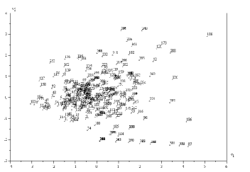
Figure 1: The feature space obtained by principal component projections of the four dimensional measurement vectors of the word association network. 

The twelve most singular nodes (i.e. words), corresponding to the respectively largest values of the Mahalanobis distances (also considering previous standardization of the measurements), are shown in decreasing order in Table 1, where the first three rows include the overall average, minimum and maximum values of the respective features.

$Word$	$k$	$a$	$r$	$cv$	$cc$	$loc$
average	5.66	9.12	2.38	0.60	0.17	0.38
minimum	1	2.00	0.18	0.00	0.00	0.09
maximum	35	21.50	10.75	1.40	1.00	0.88
183 (good)	35	6.43	0.18	0.57	0.05	0.88
186 (land)	2	21.50	10.75	0.89	1.00	0.09
106 (breath)	2	20.50	10.25	0.45	0.00	0.09
18 (long)	27	6.19	0.23	0.57	0.04	0.84
136 (service)	2	19.00	9.50	1.19	0.00	0.10
87 (saddle)	1	10.00	10.00	0.00	0.00	0.10
300 (sharp)	1	9.00	9.00	0.00	0.00	0.10
302 (bear)	1	9.00	9.00	0.00	0.00	0.10
194 (two)	24	7.08	0.30	0.64	0.07	0.81
292 (finger)	2	17.50	8.75	0.77	0.00	0.10
241 (ask)	2	3.00	1.50	0.47	1.00	0.50
265 (answer)	2	3.00	1.50	0.47	1.00	0.50

Table 1: The twelve most singular nodes obtained for the word association network and their respective non-normalized features.

For the sake of complementing the following discussion, the traditional node degrees and the non-normalized average neighboring degrees are also given in the first two columns, respectively. In addition, many of the extremal (i.e. minimum and maximum) values of each feature are present among the detected singularities. The singularities in Table 1 can be divided into groups of words as follows:

Group 1 (183, 18, 194): These singular words are characterized by relatively high values of locality index, high node degree (i.e. they are hubs), medium values of $r$ and low values of $cc$. Such properties indicate that these words are associated to many others words which are not in the immediate neighborhood. These three words appear at the left-hand extremity of the data distribution in Figure 1. Interestingly, they correspond to ‘good’, ‘long’ and ‘one’, which are adjectives.

Group 2 (186): This word not only has connectivity features which are different from all other words in Table 1, but also appears particularly isolated in the feature space (upper right-hand corner) in Figure 1. It is characterized by low degree but high neighboring degree, reflected in the highest relative neighboring degree value (10.75). It also exhibits a high coefficient of variation and maximum clustering coefficient, while the locality index is particularly low (the minimum for the network). Therefore, this word has been associated to two other words which present markedly distinct degrees and which are themselves interrelated. Not surprisingly, those two words are the common adjectives ‘good’ and ‘bad’, with respective degrees of 35 and 8. In this sense the measurement $cv$ is capable of expressing the asymmetry of the connections established by the immediate neighbors. This word is best understood as a second hierarchical level hub.

Group 3 (106, 136, 292): These three words are similar to that in Group 2 (and, as that word, are also substantives), except that they present lower clustering coefficient (i.e. the two immediate neighbors are not interconnected) and coefficient of variation (i.e. the degrees of the immediate neighbors are more uniform). These three words can be found at the lower right-hand corner of the feature space in Figure 1.

Group 4 (87, 300, 302): These words have unit degree, therefore exhibiting low $cv$, $cc$ and $loc$. These words were not exercised particularly during the experiment because they appeared near its conclusion. They can be found at the extremity of the alignment of points in the feature space in Figure 1, corresponding to other words with similar properties. Note that the own aligned group of cases is itself a mesoscopic singularity of the network.

Group 5 (241, 265): These two related verbs, ‘ask’ and ‘answer’, are characterized by having two immediate neighbors, each of them being interconnected and establishing two connections with other network nodes. Interestingly, the obtained symmetry of local connections reflected the inherently symmetry of these two words.

An additional interesting point follows that, from a theoretical point of view, each feature could have 2 kinds of outliers: those towards the minimum and those towards the maximum of that particular feature. For 4 features, there are thus $2^{4}=16$ possible groups of outliers. Looking at the word association, we find 5 groups of main outliers. Why are some groups of outliers found whereas 11 potential groups are absent? Among the several possible reasons we have that: (a) some groups are absent (skewed feature distribution) (b) some groups are present but not included in the top 12 singularities (c) some features strongly correlate with each other leading to the merger of potential outlier groups. For example, if a minimum feature A correlates with a maximum in feature B (negative correlation), outliers may form one group AB. However, if all features are statistically independent and distributions are non-skewed, all potential groups of outliers should also occur in the top list. In short, looking at absent outlier groups (a singularity of the singularity pattern) can provide additional information about the nature of the network connectivity.

The above results, which could by no means be inferred from the visual inspection of the network, illustrate the effectiviness and complementariness of the four adopted measurements in providing the basis for sound singularity detection, with good agreement between the Mahalanobis values and the distribution in the projected feature space. A series of peculiar local connectivity features were identified which allowed interesting interpretations.

It is not by chance that hubs and communities have become particularly important in complex network research: they correspond to structural singularities. In this work we extended the general principle that minority deviations are essential in order to analyze the local connectivity around each node in a network. Four complementary measurements, all stable to small perturbations (e.g. da F. Costa et al. (2006)), have been used to derive 4-dimensional informative feature vectors. Two multivariate methodologies, including visualization after standardization and principal component projections, as well as the calculation of the Mahalanobis distances in the full feature space, have been applied in order to identify the twelve most singular nodes in the word association network, which were divided into five main groups presenting distinctive properties. We are currently applying the suggested methodology to a number of other important real networks, with similarly encouraging results. Possible future works include the consideration of broader context around each node (e.g. by using the hierarchical schemes described in da F. Costa (2004a); da F. Costa and da Rocha (2006); da F. Costa and Silva (2006)) as well as the application of the method for the analysis of each detected community. Another promising work would be to consider singularity identification during network growth or dismantling (e.g. attacks). More sophisticated alternatives for outlier detection are also possible, especially by using hierarchical clustering algorithms (e.g. Duda et al. (2001); da F. Costa and Silva (2006)) in order to obtain further information about how the singularities fit in the overall network structure.

Luciano da F. Costa is grateful to CNPq (308231/03-1) and FAPESP for financial support.

References

- Marr (1980) D. Marr, Vision (Freeman, 1980).
- Kaiser and Lappe (2004) M. Kaiser and M. Lappe, Neuron 41, 293 (2004).
- Albert and Barabási (2002) R. Albert and A. L. Barabási, Rev. Mod. Phys. 74, 47 (2002).
- Newman (2003) M. E. J. Newman, SIAM Review 45, 167 (2003), cond-mat/0303516.
- Boccaletti et al. (2006) S. Boccaletti, V. Latora, Y. Moreno, M. Chavez, and D.-U. Hwang, Physics Reports 424, 175 (2006), cond-mat/0303516.
- Erdős and Rényi (1961) P. Erdős and A. Rényi, Acta Mathematica Scientia Hungary 12, 261 (1961).
- Milgram (1967) S. Milgram, Psychology Today pp. 61–67 (1967).
- Faloutsos et al. (1999) M. Faloutsos, P. Faloutsos, and C. Faloutsos, Computer Communication Review 29, 251 (1999).
- Milo et al. (2002) R. Milo, S. Shen-Orr, S. Itzkovitz, N. Kashtan, D. Chklovskii, and U. Alon, Science 298, 824 (2002).
- Sporns and Kötter (2004) O. Sporns and R. Kötter, PLoS Biology 2 e369 (2004).
- Guimerà and Amaral (2005) R. Guimerà and L. A. N. Amaral, Nature 433, 895 (2005).
- Newman (2004) M. E. J. Newman, Phys. Rev. E 69, 1 (2004).
- da F. Costa et al. (2006) L. da F. Costa, F. A. Rodrigues, G. Travieso, and P. R. V. Boas (2006), cond-mat/0505185.
- Johnson and Wichern (2002) R. A. Johnson and D. W. Wichern, Applied multivariate statistical analysis (Prentice-Hall, 2002).
- da F. Costa (2004a) L. da F. Costa, Phys. Rev. Letts. 93, 098702 (2004a).
- da F. Costa and da Rocha (2006) L. da F. Costa and L. E. C. da Rocha, Eur. Phys. J. B 50, 237 (2006).
- da F. Costa and Silva (2006) L. da F. Costa and F. N. Silva, J. Stat. Phys. (2006), in press, cond-mat/0412761.
- Kaiser and Hilgetag (2004) M. Kaiser and C. Hilgetag, Biol. Cybern. 90, 311 (2004).
- da F. Costa and Sporns (2005) L. da F. Costa and O. Sporns, Eur. Phys. J. B 48, 567 (2005).
- Duda et al. (2001) R. O. Duda, P. E. Hart, and D. G. Stork, Pattern Classification (Wiley Interscience, 2001).
- da F. Costa (2004b) L. da F. Costa, Intl. J. Mod. Phys. C 15, 371 (2004b).