Accuracy and Precision of Methods for Community Identification in Weighted Networks

Abstract

Based on brief review of approaches for community identification and measurement for sensitivity characterization, the accuracy and precision of several approaches for detecting communities in weighted networks are investigated. In weighted networks, the community structure should take both links and link weights into account and the partition of networks should be evaluated by weighted modularity $Q^{w}$. The results reveal that link weight has important effects on communities especially in dense networks. Potts model and Weighted Extremal Optimization (WEO) algorithm work well on weighted networks. Then Potts model and WEO algorithms are used to detect communities in Rhesus monkey network. The results gives nice understanding for real community structure.

Keyword: Weighted Networks, Community Structure, Similarity Function

PACS: 89.75.Hc 05.40.-a 87.23.Kg

1 Introduction

In recent years, more and more systems in many different fields are depicted as complex networks, and recent empirical studies on networks display that there are communities in social networks, metabolic networks, economic networks [1, 2, 3, 4, 5] and so on. As one of the important properties of networks, community structure attracts us much attention.

In binary networks, community structure is defined as groups of network vertices, within groups there are dense internal links among nodes, but between groups nodes loosely connected to the rest of the network[10]. Community structure is one of the most important characters to understand the functional properties of complex networks. For instance, in food web, communities reveal the subsystem of ecosystem[7]. In the world wide web, the community analysis has found thematic groups[34, 35]. Email network can be divided into departmental groups whose work is distinct and the communities reveal organization structure[8, 9]. In biochemical or neural networks, communities may correspond to functional groups[11]. The deep understanding on community structure will make us comprehend and analyze the characteristics of systems better.

In order to partition communities of networks, many approaches have been proposed recently [12, 13, 14, 15, 16, 17, 18, 19, 20, 21, 23, 24, 25, 26]. Most of these methods detect communities according to topological structure or dynamical behaviors of networks. Their sensitivity and computational cost have been investigated by Danon et al recently[27]. In practical situation, the number of communities are not known ahead of time. So to evaluate the partition of networks quantitatively is an important issue in community identification. Newman and Girvan proposed a measurement for the partition of a network based on topological structure, which is called modularity $Q$[23]. The value of modularity is lager, the partition is better.

Most of above methods are developed for binary networks. In binary networks, the closeness of relationships (link weight) among the nodes are neglected. But in many real networks, link weight plays an important rule in the structure and function of complex networks. The community identification in weighted networks could give us better understanding for the real functional groups.

For detecting community structure in weighted networks, the first problem is how to define the community structure in weighted networks. It is related with the evaluation of partitions of weighted network. In binary networks, it is enough to consider link density among nodes. But in weighted networks, the closeness of relations also affect community structure. So the definition of the community must integrate link with link weight. Newman has generalized the modularity $Q$ to weighted modularity $Q^{w}$[30]. It suggests that we can depict the community as follows: community structure is the groups of network vertices. The fraction of internal link weight among nodes within groups is much greater than that of link weight between groups. In other words, the relations among nodes within groups are much closer than relations between groups.

The second problem is that which method is more appropriate for detecting community in weighted networks. Most approaches develope for binary networks can be generalized to weighted networks. For example, in presented algorithms, GN algorithm is based on the link betweenees. When we take link weight into account, the link betweenness can be gotten from weighted shortest path[23]. Potts model algorithm is based on Potts spin glass Hamiltonian, and link weight could represent coupling strength between spins[24]. Extremal Optimization(EO) method considers the contribution of links to modularity[25]. We could generalize it to Weighted Extremal Optimization(WEO) algorithm, which will consider the contribution of link weight to weighted modularity. Usually, groups separated with the link weight should be different from the result based only on topological structure. The above three methods give us the important examples of approaches for community identification based on topological structure, dynamics, and modularity respectively. In this paper, we mainly focus on GN algorithm, Potts model and WEO method in weighted networks.

In order to find an appropriate approach on weighted networks, it is necessary to evaluate accuracy and precision of each method. We can apply each method to ad hoc networks with a well known, fixed community structure. Then accuracy can be got by comparing the presumed communities and the communities found by the algorithm. While precision can be calculated by comparing any pair of communities found by the algorithm under same conditions. Obviously, measuring the difference of different community structures quantitatively is needed to evaluate accuracy and precision. Newman described a method to calculate the sensitivity of algorithms[23]. Leon Danon et al proposed a measurement $I(A,B)$ based on information theory[27]. These two measurements mainly focus on the proportion of nodes which are correctly grouped. In our previous work, we proposed a similarity function $S$ to measure the difference between partitions[28]. It is based on the similarity and dissimilarity of two sets and addresses the difference of number of groups in different partitions. We will discuss these measurements briefly and adopt similarity function $S$ to quantify the difference of different partitions.

In this paper, we investigate the performance of several generalized approaches for detecting community structures in weighted networks. Both accuracy and precision are evaluated. The presentation is organized as follows. In Section 2, we introduce the weighted modularity and some approaches for community identification briefly. Then we review some methods to measure the difference of different communities and introduce similarity function $S$ to quantitatively describe the consistency between different partitions. Section 3 gives results of the accuracy and precision of several approaches based on idealized binary and weighted networks. The results reveal that weighted modularity $Q^{w}$ gives a nice description for the community structure of weighted networks. Potts model based approach and WEO approach work well in detecting community in weighted networks. Then WEO approach is applied to Rhesus monkey network. The result is consistent well with the real societies. Some concluding remarks are given in Section 4 .

2 Weighted Modularity, Approaches and Measurements

1. Weighted Modularity. Link weight, as a strength of interaction, is believed to be an important variable in networks. It gives more information about the network besides its topology dominated by links. Weighted networks can depict the real system better and the community structure should take link weights into account. So the definition of community[10] in weighted networks need be modified.

Newman and Girvan have defined a modularity $Q$ to evaluate community identification in binary networks[23]. Newman have indicated that modularity $Q$ can be generalized to weighted networks[30]:

$$Q^{w}=\frac{1}{2w}\sum_{ij}[w_{ij}-\frac{w_{i}w_{j}}{2w}]\delta(c_{i},c_{j}),$$ (1)

where $w_{ij}$ is the link weight (similarity weight) between node $i$ and $j$, $w_{i}=\sum_{j}w_{ij}$ (vertex weight) is the summation of link weight attaching to node $i$, $w=\frac{1}{2}\sum_{ij}w_{ij}$ is the summation of link weight in the network, and $c_{i}$ shows that vertex $i$ belongs to community $c_{i}$. Hence Eq. (1) can be write as

$$Q^{w}=\sum_{r}(e^{w}_{rr}-(a^{w}_{r})^{2})$$ (2)

where $e^{w}_{rr}=\frac{1}{2w}\sum_{ij}w_{ij}\delta(c_{i},r)\delta(c_{j},r)$ is the fraction of summation of link weight that connect two nodes inside the community $r$, $a^{w}_{r}=\frac{1}{2w}\sum_{i}w_{i}\delta(c_{i},r)$ is the fraction of summation of vertex weight of community $r$. Obviously, $Q^{w}$ takes both link and link weight into account. It suggests a description for community in weighted networks. We think that weighted community structure is the groups of network vertices. The summation of internal link weight among nodes within groups are larger than that of link weight between groups. In other words, the relations of nodes within group are close, but the relations of nodes between groups are distant. In the following discussion, we evaluate a partition of weighted networks by the weighted modularity $Q^{w}$ given by Eq. (2) and $Q^{w}$ is considered as the global variable to optimize in extremal optimization algorithm.

2. Methods for Detecting Community. In this paper, we mainly discuss the the performance of GN algorithm, Potts model algorithm, and Extremal Optimization algorithm in weighted networks.

The GN algorithm is based on the concept of edge betweenness. The betweenness of an edge in network is defined to be the number of the shortest paths passing through it. It is very clearly that edges which connect communities, as all shortest paths that connect nodes in different communities have to run along it, have a larger betweenness value. By removing the edge with the largest betweenness at each step, the whole network can be gradually split into isolated components or communities[10]. Based on weighted shortest path, the above ideas can be easily generalized to weighted networks[30].

For Potts model algorithm, community coincides with the domain of equal spin value in the minima of modified Potts spin glass Hamiltonian. The node in networks just be looked as the electron with spin elected from $q$ spin states. The link correspond to the reciprocity between electrons. This will allow us to partition the communities of a network onto the magnetic domains in the ground state or in local minima of a suitable Hamiltonian. For this purpose authors[24] append a global constraint to the q-state Potts Hamiltonian that forces the spins into communities according to

$$H=\sum_{(i,j)\in E}J_{ij}\delta_{\sigma_{i}\sigma_{j}}+\gamma\sum_{s=1}^{q}\frac{n_{s}(n_{s}-1)}{2}$$ (3)

where, $\sigma_{i}$ denotes the individual spins which are allowed to take $q$ values $1...q$, $n_{s}$ denotes the number of spins that have spin $s$ such that $\sum^{q}_{s=1}n_{s}=N$, $J_{ij}$ is the ferromagnetic interaction strength, $\gamma=\frac{2<J_{ij}>M}{N(N-1)}$ is a positive parameter. To practically find or approximate the ground state of system, a simple Metropolis algorithm could be employed. For weighted networks, $J_{ij}$ can be taken as similarity link weight. Then Potts model algorithm can be easily applied to weighted networks.

The Extremal Optimization algorithm uses a heuristic search to optimize the modularity $Q$ by dividing network into groups[25]. When this method is generalized to weighted networks, $Q$ is replaced by $Q^{w}$ as the global variable to optimize. While the value of each node contributing to weighted modularity $Q^{w}$ can be defined as

$$q^{w}_{i}=w_{r(i)}-w_{i}a^{w}_{r(i)},$$ (4)

where $w_{r(i)}$ is the summation of link weight that a node $i$ belonging to a community $r$ has with nodes in the same community, and $w_{i}$ is the vertex weight of node $i$. So the modularity $Q^{w}$ is $Q^{w}=\frac{1}{2w}\sum_{i}q^{w}_{i}$. Rescaling the local variable $q^{w}_{i}$ by the vertex weight of node $i$, the contribution of node $i$ to the weighted modularity is defined as

$$\lambda^{w}_{i}=\frac{q^{w}_{i}}{w_{i}}=\frac{w_{r(i)}}{w_{i}}-a^{w}_{r(i)},$$ (5)

$\lambda^{w}_{i}$ is normalized in the interval $[-1,1]$. It gives the relative contributions of individual nodes to the community structure. So it could be considered as the fitness of a node involved in the weighted extremal optimization process. The process of detecting community structure by weighted extremal optimization (WEO) is as follows:

1. Initially, split randomly the whole network into two groups with similar number of nodes.

2. At each time step, move the node with the lower fitness from one group to the other. After each movement, recalculate the fitness of every node based on Eq. (5).

3. Repeat process $2$ until a maximum value of $Q^{w}$ is reached. After that, proceed recursively with every group. When the modularity $Q^{w}$ cannot be improved, the process will finish.

In order to escape from local maxima, WEO algorithm adopts $\tau$-EO method[36]. The node is selected according to the following probability:

$$P(q)\propto q^{-\tau},$$ (6)

where $q$ is the rank number of node according to their fitness values, and $\tau\sim 1+1/ln(N)$.

3. Comparing Two Community Structures. In order to find appropriate method to solve a certain problem, we should know the performance of each method, including their speed and sensitivity. Usually the sensitivity of a algorithm is tested by its performance when it is applied to ad hoc networks with a well known, fixed structure. The previous researches focus only on the accuracy of a method. Here we address that both accuracy and precision of a algorithm should be examined. When we proceed the methods several times under the same condition, they may give different community structures due to the random factors in the algorithm. Instead of comparing with the presumed communities to get the accuracy, the precision should be got by comparing the results from different runs under the same conditions. Obviously, in order to get accuracy or precision of a method, we need to quantify the differences between different community structures. In other words, we need a measurement to evaluate the similarity between communities.

There are already several methods to quantify the difference of different partitions. Newman described a evaluating method in [23]. The largest set of vertices grouped together in each of the four known communities is considered correctly classified. If two or more of known sets are put into the same group, then all vertices in those sets are considered incorrectly classified. All other vertices not in the largest sets are considered incorrectly classified. Leon Danon et al proposed the use of the normalized mutual information measure[27]. It is based on the confusion matrix $N$, where the rows denote the presumed communities before divided, and the columns correspond to the communities found by some algorithm. The matrix element($N_{ij}$) of $N$ is the number of nodes in the presumed community $i$ that appear in the found community $j$. A measure of similarity between the partitions, based on information theory, is then:

$$I(A,B)=\frac{-2\sum^{c_{A}}_{i=1}\sum^{c_{B}}_{j=1}N_{ij}\log(\frac{N_{ij}N}{N_{i.}N_{.j}})}{\sum^{c_{A}}_{i=1}N_{i.}\log(\frac{N_{i.}}{N})+\sum^{c_{B}}_{j=1}N_{.j}\log(\frac{N_{.j}}{N})}$$ (7)

where $c_{A}$ is the number of presumed communities and $c_{B}$ is the number of found communities, $N_{i.}$ is the sum over row $i$ of matrix $N_{ij}$ and $N_{.j}$ is the sum over column $j$.

The above two measurements mainly focus on the proportion of nodes which have been grouped correctly. We have also suggested a method to characterize the difference of community structures quantitatively[28]. It is based on the similarity and dissimilarity of two sets $A$ and $B$ defined as the subset of $\Omega=A\bigcup B$. The normalized similarity are defined as

$$s=\frac{\left|A\cap B\right|}{\left|A\cup B\right|}\\$$ (8)

Given any two partitions, we should first construct correspondence between two subsets of two partitions. Then we can get similarity function $S$ by integrating the results of every single pair[28].

The former two methods evaluate the sensitivity of algorithm by measuring the percentage of nodes divided correctly, while the similarity function $S$ we proposed emphasize the difference of communities. In our method, all clusters have equal status regardless of its size. For a network with 128 nodes and 4 presumed groups with 32 nodes each, if there are three communities divided by a method, two of which correspond exactly to two original communities, and a third, which corresponds to the other two clustered together, the similarity is $S=0.625$, Newman’s measurement gives 0.5, and $I(A,B)=0.858$. Considering another example, a network consists of $n=20$ vertices and is divided into two presumed groups of $10$ nodes each. It is provided by a method that there are three communities in the result. The two largest groups are divided correctly except one node which forms the third group. In this case, the accuracy given by each measurements are $0.95$(Newman), $0.9$ ($I(A,B)$), and the similarity function is $0.63$. So our method for quantifying the difference of partitions emphasizes the number of communities. It is a reasonable evaluating index to quantify the difference of community structures. In the following discussion, we use $S$ to describe the accuracy and precision of the approaches.

3 Results Based on Idealized Networks and Empirical Studies

The above methods will be applied to ad hoc networks firstly introduced by Newman and used by many other authors[23, 27]. Each network consists of $n=128$ vertices, which divided into four groups of $32$ nodes. Vertices are assigned to groups and are randomly connected to vertices of the same group by an average of $\langle k_{in}\rangle$ links and to vertices of different groups by an average of $\langle k_{out}\rangle$ links. The average degree of all vertices are fixed, namely $\langle k_{in}\rangle+\langle k_{out}\rangle=16$. With $\langle k_{out}\rangle$ increasing from small, the communities become more and more diffuse, and it becomes more and more difficult to detect the communities. Since the community structure is well known in this case, it is possible to measure accuracy and precision of each method by quantifying the difference of partitions.

For each approach of community identification, accuracy could be gotten by the comparison between the divided communities with the presumed one and precision should be gotten by the comparison between any pair of results, which are found by same algorithm performing several times on the same network. In the following numerical investigations, we first get $20$ realizations of idealized ad hoc networks under the same conditions. Then we run each algorithm to find communities in each network $10$ times. Based on these results, using the similarity function $S$, comparing each pair of these $10$ community structures and average over the $20$ networks (average of $900$ results) could give us the precision of the algorithm. Comparing each divided groups with the presumed structure, we can get the accuracy of the algorithm by averaging these $200$ results.

3.1 Results for binary networks

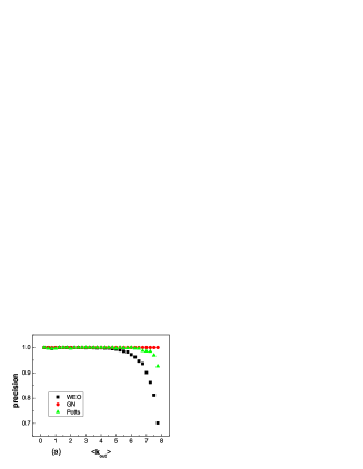
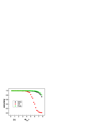
Figure 1: Algorithm performance as applied to ad hoc networks with $n=128$ and four communities of 32 nodes each. Total average degree is fixed to 16. (a)Comparing precision of the algorithm by several results on same ad hoc networks. (b)Comparing accuracy using ad hoc networks with presumed community structure. The x-axis is the average of connections to outside communities $\langle k_{out}\rangle$. Each point is an average over $20$ networks and $10$ runs each.

We apply GN, Potts model, and WEO algorithm on binary ad hoc network first and focus on both accuracy and precision of the methods measured by similarity function $S$. From the results shown in Fig.1, when $\langle k_{out}\rangle$ is small, they could find communities well and truly. The communities become more diffuse with $\langle k_{out}\rangle$ increasing. Once $\langle k_{out}\rangle$ is lager than a certain value, it is difficult to find presumed communities exactly. For small $\langle k_{out}\rangle$, there are no discrimination between results of any algorithms. But for large $\langle k_{out}\rangle$, the precision of different algorithms is various (Fig.1(a)) and accuracy falls across the different algorithms. For example, GN algorithm is stable for any $\langle k_{out}\rangle$, though its accuracy is worse when $\langle k_{out}\rangle$ is large. However, Potts model and EO algorithm are fluctuant, though their accuracy are better.

As shown in Fig.1(b), with $\langle k_{out}\rangle$ increasing, accuracy of GN algorithm described by similarity function $S$ decline more quickly than the other measurements. It is because there are many small clusters in found communities by GN algorithm and similarity function $S$ addresses the number of communities crucially.

3.2 Results based on weighted ad hoc networks

In this section, ad hoc networks is added similarity link weight to describe the closeness of relations. Similarity weight is proportional to the closeness of relationships. The larger the link weight is, the closer the relation is. Under the basic construction of ad hoc network described above, the weight of link connected to vertices of the same group is assigned as $1$, while the weight of link connected to vertices of different groups is assigned as $w_{out}$. In practise, the relationship among the nodes in groups is usually more closer than the relationship between groups. So $w_{out}$ is normally less than 1. When $w_{out}$ is equal to $1$, weighted ad hoc network could be seen as a binary one.

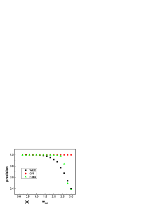
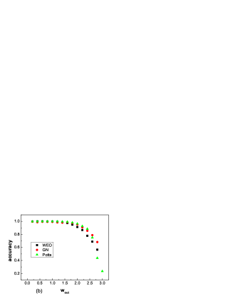
Figure 2: Networks with $\langle k_{out}\rangle$ equaling to $4$. The link weights among the nodes in groups are fixed to 1. The influence of link weight on the out edge on precision(a) and accuracy(b) when out link weight changes from $0.2$ to $3$. Each point is an average over $20$ networks and $10$ runs each.

We consider weighted modularity $Q^{w}$ as the criteria to evaluating partition of communities. Though there are only two kinds of link weight value in weighted ad hoc networks, the role of weight on community structure can be investigated qualitatively. When $\langle k_{out}\rangle$ is fixed, with $w_{out}$ increasing from small, it affects community structure obviously.

When $\langle k_{out}\rangle$ is equal to $4$, any methods can easily partition communities for binary networks. When $w_{out}$ is small or even equals 1, all algorithms works well to get the correct communities (as shown in Fig.2). When $\langle k_{out}\rangle$ is small, we know that the community structure is dominated by links. So we can find the presumed groups even when $w_{out}$ is larger than 1.

In other hand, when $\langle k_{out}\rangle$ is large, the communities is very diffuse in binary networks and it is impossible to find communities correctly by any algorithms. But now the link weight plays a crucial role in the partition of communities. When $w_{out}$ is small, the network can also be partitioned accurately into presumed communities (shown as Fig.3). In this case, Potts model and WEO algorithm work better than GN algorithm. Although GN algorithm has nice precision, it gives results in low accuracy.

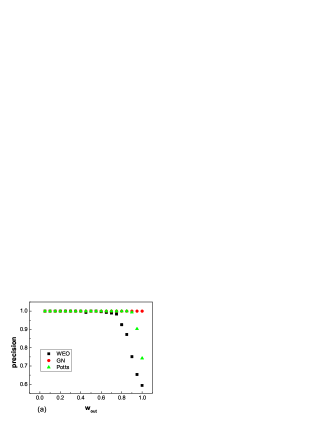
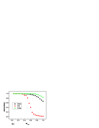
Figure 3: The influence of weight on community structure when $\langle k_{out}\rangle$ is equal to $8$. A series of networks possess identical topological structure, and out link weight changes from $0.05$ to $1$. Each point is an average over $20$ networks and $10$ runs each.

From the above results, we can see that topology and link weight are two factors that affect community structure. When we set $w_{out}$ equal 0.2, Fig.6 shows the precision and accuracy of Potts model and WEO algorithm as the function of $\langle k_{out}\rangle$. The spectrum of $\langle k_{out}\rangle$ is lager than that of binary networks. The results show the link weight really plays an important rule in community structure and the Potts model and WEO methods are effective in detecting communities in weighted networks. Even in complete networks, when we set the link weight be $1$ among the same presumed group, while the link weight is $w_{out}$($w_{out}<1$) between groups, these two algorithms can divided the network into communities correctly (as shown in Fig.5). In dense networks, link weight is more important than in sparse networks. So weighted modularity $Q^{w}$ and corresponding algorithms are helpful to detecting community structure in dense weighted networks.

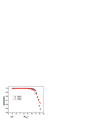
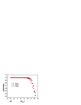
Figure 4: The influence of topology on community structure when $w_{out}$ is fixed as $0.2$. Each point is an average over $20$ networks and $10$ runs each.

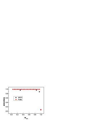
Figure 5: Accuracy of Potts and WEO algorithms in complete networks with presumed communities. When $w_{out}$ is less than 1, the algorithms can find the groups correctly. Each point is an average over $10$ runs.

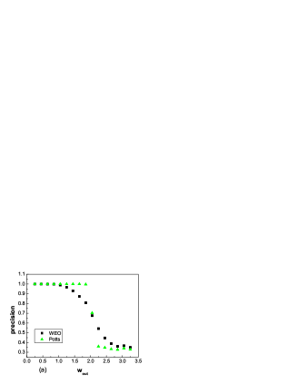
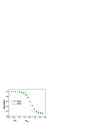
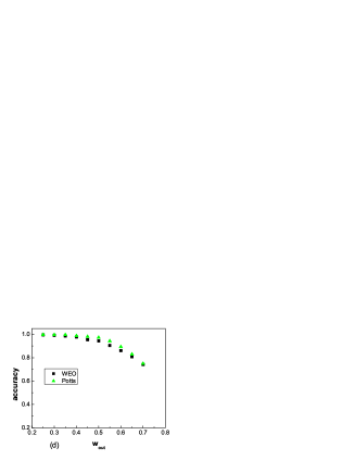
Figure 6: The performance of Potts model and WEO algorithms in networks with randomly distributed link weights. (a) and (b) are the precision and accuracy of the algorithms when $\langle k_{out}\rangle$ is equal to $4$. (c) and (d) are the results when $\langle k_{out}\rangle$ is equal to $8$. Each point is an average over $20$ networks and $10$ runs each.

In real weighted networks, link weights are usually randomly distributed. We have also tested Potts model and WEO algorithm in the idealized ad hoc networks with random link weight distribution. For a given network topology with certain $\langle k_{out}\rangle$, weights in links among groups are taken randomly from [0.5,1]. The average link weight in groups is 0.75. While weights in links between groups ($w_{out}$) are also taken randomly from a interval with the same length. With the changing of its average value, we can also get the performance of algorithms under different conditions. The results are summarized in Fig.6. They are qualitatively similar with the above results.

3.3 Community structure in Rhesus monkey network

The above investigations are based on idealized networks. Now we move to some real weighted networks. One example is Rhesus monkey network which is studied by Sade[29] in $1972$. This network is based on observations of group F Cayo Santiago, in which $38$ monkeys comprise $6$ genealogies and $2$ non-natal males ($066$ and $R006$). The grooming episodes of monkeys were registered between $14th$ June and $31st$ July $1963$, just prior to the mating season on Cayo Santiago. The network showed the information of members, who were $4$ years old or older in $1963$. Links denote grooming behavior between the monkeys and link weight is the number of instances of grooming of each monkey by each other during the period of observation. The network has $16$ vertices and $69$ links with link weights ranging from $1$ to $49$.

Newman has illuminated its community structure by weighted GN algorithm (See Fig.2 (b) in [30]). Here we test Potts model and WEO algorithm in Rhesus monkey network. Two algorithms have been applied 20 times to get the communities. Their precision measured by similarity function are: 0.95(Potts) and 1.00(WEO) respectively. The final community structures are shown in Fig.7. Fig.7(a) shows the result gotten by Potts model algorithm. The network is partitioned into 4 groups. Its $Q^{w}$ is 0.23. By WEO algorithm, the network is divided into three communities(A, C and D). Firstly, rhesus monkey network is partitioned into two groups(A and B), then group B is divided into two smaller groups (Fig.7), and the max weighted modularity $Q^{w}$ is $0.244$. $Q^{w}$ for partition (4 groups) in [30] gotten by GN method is 0.12. We have applied WEO algorithm further and have divided group $A$ and $D$ into two smaller groups. The community structures gotten by Potts and WEO algorithm are different from the results gotten by GN methods. The similarity of these communities given by similarity function $S$ are: 0.65(WEO vs. Potts), 0.22(WEO vs. GN), and 0.36(Potts vs. GN). By the detailed investigation, it could be found that results gotten by WEO and Potts model methods accord more details of the known organization of these monkeys.

From the record by Sade[29], Male $006$ had been dominant in group since at least $1960$. Male $R006$ had been solitary in $1962$, and joined this group in early $1963$. $R006$ replaced $006$ as dominant male in the fall of $1963$.

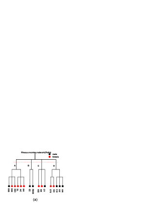
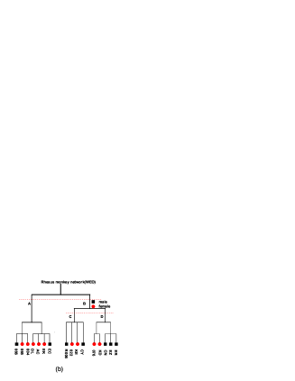
Figure 7: (a)Community structure of rhesus monkeys network gotten by Potts model. It is the result occurs with maximum probability. (b) Groups gotten by WEO algorithm. $DL$ and $EC$ were $AC$’s offspring, $CY$ and $KE$ were $022$’s offspring, and $EZ$ and $ER$ were brothers.

Based on the investigation of cliques, the following details can be known. The dominant male $066$ was co-cliqual with the first and second dominant females. $EC$, a 4-year-old male, is co-cliqual with his mother $AC$ and sister $DL$. The $4$ multi-cliqual monkeys, $065$, $004$, $AC$ and $DL$, were the $4$ highest ranking females and they formed the core of the grooming network. (This can be reflected by community A.) $EZ$ occurs only in his brother $ER$’s clique. $CN$, the adult male castrate, is co-cliqual with his mother and sister, overlapped more extensively with the cliques containing the other natal males (community D can show this detail), and might link their clique to the main group. $R006$, the new-natal male, at last did not clique with the dominant and third ranking females, $065$ and $AC$ and $AC$’s son $EC$. (This can be reflected by community C.) In conclusion, the dominant male $066$, was integrated into the core with the females. The new male, $R006$, was distantly attached to the core of females. one sub-adult male, $EC$, was still integrated into his genealogy. The other natal males formed a distinct sub-group. $CN$, the castrate, was intermediate in his position, which overlapped that of the natal males and the female core. The community structure found by WEO algorithm can illuminate above details well. This example suggests that WEO algorithm is effective at finding community structure in weighted networks.

4 Concluding Remarks

In this paper, we focus on the identification of community structure in weighted networks. When link weight is taken into account, the closeness of relations among the nodes in a group should be characterized both by link and link weight. Weighted modularity $Q^{w}$ should be taken as the criteria for partition of communities. A brief overview of some partition algorithm is given including the introduction of local variable $\lambda^{w}_{i}$ of weighted network in the external optimization process. In addition, we review the methods to evaluate accuracy and precision of different algorithms and present similarity function $S$, a measurement to quantify the difference of different communities. In weighted ad hoc networks, we study the influence of weight on the process of detecting community structure and find that the change of link weight can affect the accuracy and precision of algorithms. When community structure is dominated by topological linkage, GN algorithm works better than other algorithms. But for dense networks, when link weight plays more important rule in network properties, Potts model and WEO algorithm works better to get the correct communities. At last, we use WEO algorithm to Rhesus monkey network. The results show that community identification with weighted modularity $Q^{w}$ and WEO algorithm gives better understanding for real networks.

From these investigations, we could find that the role of weight on the weighted networks could be investigated by studying the effect of weight on the community structure. For weighted networks, the disturbing of distribution or matching between weights and edges should have some important effects on community structure. So the community structure in networks should be a suitable property for investigating the role of weight.

References

- [1] Michelle Girvan, M. E. J. Newman, Proc. Natl. Acad. Sci. USA 99, 7821-7826 (2002)
- [2] Boss M, Elsinger H, Summer M and Thurner S, Preprint cond-mat/0309582.
- [3] Ravasz E, Somera A L, Mongru D A, Olvai Z N and Barabási A L, 2002, Science, 297, 1551.
- [4] Guimerà R, Amaral L A N, 2005, Nature, 433, 895-900.
- [5] Holme P, Huss M and Jeong H, 2003, Bioinformatics, 19, 532.
- [6] P. Gleiser, L. Danon, Advances in Complex Systems, 6 (2003) 565-573.
- [7] R. J. Williams, N. D. Martinez, Nature 404 (2000) 180-183.
- [8] Joshua R. Tyler, Dennis M. Wilkinson, Bernardo A. Huberman, arXiv:cond-mat/0303264.
- [9] R. Guimerà, L. Danon, A. Díaz-Guilera, F. Giralt, A. Arenas, Phys.Rev. E 68 (2003) 065103.
- [10] M. Girvan, M.E.J. Newman, Proc. Natl. Acad. Sci. 99 (2002) 7821-7826.
- [11] Zhou H and Lipowsky R, 2004, Lecture Notes Comput. Sci. 3038, 1062 -1069.
- [12] M. Fiedler, Czech. Math. J. 23 (1973) 298 ; A. Pothen, H. Simon, K.-P. Liou, SIAM J. Matrix Anal. Appl. 11 (1990) 430.
- [13] B.W. Kernighan, S. Lin, Bell Sys. Techn. J. 49 (1970) 291.
- [14] M.E.J. Newman, Eur. Phys. J. B 38 (2004) 321-330.
- [15] J. Scott, Sage, London, 2000, 2nd ed.
- [16] Maxwell Young, Jennifer Sager, Gábor Csárdi, Péter Hága, arXiv:cond-mat/0408263.
- [17] A. Capoccia, V.D.P. Servedioa, G. Caldarellia, F. Colaiori, Physica A 352 (2005) 669-676.
- [18] Seung-Woo Son, Hawoong Jeong, Jae Dong Noh, arXiv:cond-mat/0502672.
- [19] F. Wu, B.A. Huberman, Eur. Phys. J. B 38 (2004) 331-338.
- [20] Luca Donetti, Miguel A. Muñoz, J. Stat. Mech. P (2004) 10012.
- [21] H. Zhou, Phys. Rev. E 67 (2003) 061901.
- [22] Guimerà R and Amaral L A N, 2005, J. Stat. Mech., P02001.
- [23] M.E.J. Newman, M. Girvan, Phys.Rev. E 69 (2004) 026113.
- [24] Jörg Reichardt, Stefan Bornholdt, Phys Rev Lett. 93 (2004) 218701.
- [25] Jordi Duch and Alex Arenas, Phys Rev E. 72. 027104(2005).
- [26] M. E. J. Newman, Fast algorithm for detecting community structure in networks, Phys Rev E. 69. 066133(2004).
- [27] Leon Danon, Albert Díaz-Guilera, Jordi Duch and Alex Arenas, arXiv:cond-mat/0505245.
- [28] Peng Zhang, Menghui Li, Jinshan Wu, Zengru Di, Ying Fan, Physica A 367(2006) 577-585.
- [29] D. S. Sade, Folia Primatologica 18, 196-223 (1972).
- [30] M.E.J. Newman, Phys. Rev. E 70 (2004) 056131.
- [31] Y. Fan, M. Li, J. Chen, L. Gao, Z. Di, J. Wu, International Journal of Modern Physics B, 18 (2004) 2505-2511.
- [32] M. Li, Y. Fan, J. Chen, L. Gao, Z. Di, J. Wu, Physica A 350 (2005) 643-656.
- [33] L. Freeman, Sociometry 40 (1977) 35.
- [34] Eckmann J-P and Moses E, 2002, Proc. Natl. Acad. Sci., 99, 5825.
- [35] Zhou H and Lipowsky R, 2004, Lecture Notes Comput. Sci. 3038, 1062 - 1069.
- [36] S. Boettcher and A. G. Percus, Phys. Rev. Lett. 86, 5211(2001).