Stirring up trouble:
Multi-scale mixing measures for steady scalar sources

Abstract

The mixing efficiency of a flow advecting a passive scalar sustained by steady sources and sinks is naturally defined in terms of the suppression of bulk scalar variance in the presence of stirring, relative to the variance in the absence of stirring. These variances can be weighted at various spatial scales, leading to a family of multi-scale mixing measures and efficiencies. We derive a priori estimates on these efficiencies from the advection–diffusion partial differential equation, focusing on a broad class of statistically homogeneous and isotropic incompressible flows. The analysis produces bounds on the mixing efficiencies in terms of the Péclet number, a measure the strength of the stirring relative to molecular diffusion. We show by example that the estimates are sharp for particular source, sink and flow combinations. In general the high-Péclet number behavior of the bounds (scaling exponents as well as prefactors) depends on the structure and smoothness properties of, and length scales in, the scalar source and sink distribution. The fundamental model of the stirring of a monochromatic source/sink combination by the random sine flow is investigated in detail via direct numerical simulation and analysis. The large-scale mixing efficiency follows the upper bound scaling (within a logarithm) at high Péclet number but the intermediate and small-scale efficiencies are qualitatively less than optimal. The Péclet number scaling exponents of the efficiencies observed in the simulations are deduced theoretically from the asymptotic solution of an internal layer problem arising in a quasi-static model.

I Introduction

Mixing processes in fluids play a key role in a wide variety of engineering applications and for natural systems such as the ocean and atmosphere. Their theoretical study has been a major focus of research, as indicated by the large number of review articles Ottino1990 ; Majda1999 ; Warhaft2000 ; Shraiman2000 ; Sawford2001 ; Falkovich2001 ; Aref2002 ; Wiggins2004 . At the smallest scales mixing is achieved by molecular diffusion processes, but it may be facilitated greatly by stirring. The result of stirring is usually to enhance the effect of molecular diffusion and increase the mixing rate Batchelor1949 ; Batchelor1952a ; Batchelor1959 ; Kraichnan1968 ; Kraichnan1974 . Quantitative understanding of the fundamental features of stirring and its influence on mixing processes is important for the effective modeling, simulation and design or control of these systems.

The “efficiency” of mixing means different things in different contexts. For example the dispersion of an initial distribution by an imposed flow is a transient problem where the temporal approach to the final fully mixed state, rather than the final state itself, is of central interest. Consider for definiteness the homogeneous advection–diffusion equation for a passive scalar field $\theta(\bm{x},t)$ stirred by a divergence-free velocity field $\bm{u}(\bm{x},t)$,

$$\frac{\partial\theta}{\partial t}+\bm{u}\cdot\nabla\theta=\kappa\Delta\theta$$ (I.1)

where $\kappa$ is the molecular diffusivity. If this equation is supplied with initial concentration $\theta(\bm{x},0)$ and applied in an appropriate domain without sources, sinks or scalar flux at the boundaries, then the integral of $\theta$ is conserved, so without loss of generality it may be taken to vanish from the start. But the $L_{2}$-norm $\|\theta(\cdot,t)\|_{2}$, proportional to the scalar variance in finite volume domains, decreases with time. Indeed, multiplying (I.1) by $\theta$ and integrating by parts,

$$\frac{d}{dt}\|\theta\|_{2}^{2}=-2\kappa\|\nabla\theta\|_{2}^{2},$$ (I.2)

indicating an inexorable decay of the variance. Efficient mixing in this transient decay problem means faster decay of the scalar variance. The mixing efficiency of a particular flow could be defined, for example, in terms of its ability to reduce the variance from the initial value to a prescribed value within a specific period of time Constantin2005 . Because the right-hand side of (I.2) is proportional to $\kappa$, it is evident that molecular processes are ultimately responsible for mixing by this criterion. Even though the stirring field does not appear explicitly in (I.2), the conventional intuition is that material line stretching in the flow can amplify scalar gradients thereby enhancing the molecular mixing rate. Indeed, the velocity’s rate-of-strain matrix serves as the local growth rate of the scalar gradient field. These issues are of extreme interest for both theory and applications, but in this paper we are interested in a distinct scenario where different effects are at work.

Mixing a scalar field whose fluctuations are constantly replenished by steady but spatially inhomogeneous sources and sinks is a problem with a long history. Early on, Townsend Townsend1951 ; Townsend1954 was concerned with the effect of turbulence and molecular diffusion on a line-source of temperature, a heated filament. The spatial localization of the source, imposed by experimental constraints, enhanced the role of molecular diffusivity. Saffman Saffman1960 also found that molecular diffusion and turbulent diffusion were not simply additive and that higher-order corrections were needed. Durbin Durbin1980 and Drummond Drummond1982 introduced stochastic particle models to turbulence modeling, and these allowed more detailed studies of the effect of the source on diffusion. Sawford and Hunt Sawford1986 pointed out that small sources, such as heated filaments, lead to an explicit dependence of the variance on molecular diffusivity. Many refinements to these models followed, see for instance Thomson1990 ; Borgas1994 and the review by Sawford Sawford2001 . Chertkov et al. Chertkov1995 ; Chertkov1995b ; Chertkov1997 ; Chertkov1997b ; Chertkov1998 and Balkovsky & Fouxon Balkovsky1999 treated the case of a random, statistically-steady source. Our goal in the present paper is to make the source-dependence of the concentration variance more precise by working directly from the advection–diffusion equation, without specifying the underlying turbulent statistics other than basic stationarity and homogeneity assumptions.

When a source of scalar concentration is present, the transient kinetics are of less immediate interest and instead the properties of the (statistical) steady state are of greater relevance. As will be seen, this sustained steady-state dynamics highlights other features of stirring and mixing processes. In comparing the steady-state problem to the transient problem defined by Eq. (I.2), it is important to remember that the long-time asymptotic behavior of the decaying problem is usually irrelevant to the corresponding long-time behavior of the steady-state problem. This is because the continuous replenishing of concentration overwhelms small-amplitude effects observed for long-time decay, such as the ‘strange eigenmode’ Pierrehumbert1994 ; Antonsen1996 ; Rothstein1999 ; Fereday2002 ; Sukhatme2002 ; Wonhas2002 ; Pikovsky2003 ; Thiffeault2003d ; Thiffeault2004b ; Schekochihin2004 ; Vanneste2005 ; Gilbert2006 .

In this paper we consider the stirring and mixing of a passive scalar sustained by a steady source-sink function $s(\bm{x})$. Given a prescribed divergence-free velocity field $\bm{u}(\bm{x},t)$ and a molecular diffusivity $\kappa$, the scalar concentration $\theta(\bm{x},t)$ obeys the inhomogeneous advection–diffusion equation

$$\frac{\partial\theta}{\partial t}+\bm{u}\cdot\nabla\theta=\kappa\Delta\theta+s(\bm{x})$$ (I.3)

supplemented with initial concentration field $\theta(\bm{x},0)$. We consider a domain without any net scalar flux at the boundaries: the periodic box of size $L$, i.e., $\bm{x}\in\mathbb{T}^{d}$, the $d$-dimensional torus of volume $L^{d}$. The spatial mean of $\theta$ is computed immediately,

$$\frac{1}{L^{d}}\int\theta(\bm{x},t)\,\mathrm{d}^{d}x\ =\ \frac{1}{L^{d}}\int\theta(\bm{x},0)\,\mathrm{d}^{d}x\ +\ t\times\frac{1}{L^{d}}\int s(\bm{x})\,\mathrm{d}^{d}x\,,$$ (I.4)

and deviations from the spatial mean satisfy (I.3) with $s(\bm{x})$ replaced by $s(\bm{x})-L^{-d}\int s\,\mathrm{d}^{d}y$. So to study the fluctuations we may assume without loss of generality that $\theta(\bm{x},0)$ and $s(\bm{x})$, and thus also $\theta(\bm{x},t)$ have spatial mean zero.

Fluctuations in the scalar concentration are natually measured in terms of the steady-state variance $\langle\theta^{2}\rangle$, where we introduce the space-time average. The two averaging operations we use are the time average

$$\overline{F}(\bm{x})\mathrel{\raisebox{0.29707pt}{:}\!\!=}\lim_{t\rightarrow\infty}\frac{1}{t}\int_{0}^{t}F(\bm{x},t^{\prime})\,dt^{\prime},$$ (I.5)

assuming as necessary that the limit exists, and the space-time average

$$\langle F\rangle\mathrel{\raisebox{0.29707pt}{:}\!\!=}\frac{1}{L^{d}}\int\overline{F}(\bm{x})\,\mathrm{d}^{d}x\,.$$ (I.6)

Effective stirring makes the scalar field more spatially uniform, lowering the variance, and this is the basic mixing effect that we set out to study. Many investigations have been concerned with other statistical properties of the scalar field for this kind of model, such as details of the tails of the probability distribution of $\theta$ Majda1999 ; Falkovich2001 . While these studies present fascinating mathematical and physical issues, in terms of applications they are most likely to be of ultimate use in designing closure approximations, i.e., models of the model, in order to accurately estimate bulk measures of mixing like variance reduction. In this work we focus directly on the supression of the scalar fluctuations as a primary indicator of mixing.

In terms of the Fourier decomposition of the scalar field,

$$\hat{\theta}_{\bm{k}}(t)=\frac{1}{L^{d}}\int\theta({\bm{x}},t)\,e^{-i\bm{k}\cdot\bm{x}}\,\mathrm{d}^{d}x$$ (I.7)

where ${\bm{k}}=(2\pi/L){\bm{n}}$ for ${\bm{n}}=(n_{1},\ldots,n_{d})\in\mathbb{Z}^{d}$, the steady-state variance is

$$\langle\theta^{2}\rangle=\sum_{\bm{k}}\overline{|\hat{\theta}_{\bm{k}}|^{2}}.$$ (I.8)

The magnitude $k$ of the wavenumbers naturally index spatial scales, so information about the fluctuations at different scales may be obtained by weighting the sums of the Fourier coefficients Mathew2005 . The simplest indicators of the fluctuations on small and large scales are, respectively,

$$\langle|\nabla\theta|^{2}\rangle=\sum_{\bm{k}}k^{2}\overline{|\hat{\theta}_{\bm{k}}|^{2}}$$ (I.9)

and

$$\langle|\nabla^{-1}\theta|^{2}\rangle=\sum_{\bm{k}}\overline{|\hat{\theta}_{\bm{k}}|^{2}}/k^{2}$$ (I.10)

where the inverse gradient $\nabla^{-1}$ is defined in Fourier space as multiplication by $-i{\bm{k}}/k^{2}$, a well-defined operator on these functions with spatial mean zero. For the purposes of this study the effectiveness of stirring on mixing at relatively small and large scales will be gauged in terms of these norms. Efficient stirring decreases the variances on all scales, although it can be expected that any particular stirring may be more effective on some scales than on others.

It is appropriate here to point out a fundamental and elementary distinction between transient and steady-state stirring. For efficient transient mixing the goal is to decrease the scalar variance $\sim\|\theta(\cdot,t)\|_{2}^{2}$ as quickly as possible by increasing the gradient variance $\sim\|\nabla\theta(\cdot,t)\|_{2}^{2}$ via stirring. However in the steady-state problem stirring can only reduce the mean scalar gradient variance—and thus the mean rate of variance decay—from its purely diffusive value in the absence of stirring.

The proof of this (perhaps unexpected) fact is easy. Multiplying (I.3) by $\theta$ and averaging over space and time with appropriate integrations by parts produces the well-known balance

$$\kappa\langle|\nabla\theta|^{2}\rangle=\langle\theta s\rangle.$$ (I.11)

Inserting the gradient and its inverse on the right-hand side, integrating by parts again, and then employing the Cauchy–Schwarz inequality yields

$$\kappa\langle|\nabla\theta|^{2}\rangle\ =\ \langle\theta\nabla\cdot\nabla^{-1}s\rangle\ =\ -\langle\nabla\theta\cdot\nabla^{-1}s\rangle\ \leq\ \langle|\nabla\theta|^{2}\rangle^{1/2}\langle|\nabla^{-1}s|\rangle^{1/2}.$$ (I.12)

Note that the long-time solution of (I.3) in the absence of stirring is the steady-state solution $\theta_{0}(\bm{x})$ of the diffusion equation with source $s(\bm{x})$,

$$\theta_{0}\ =\ -\frac{1}{\kappa}\Delta^{-1}s\,,$$ (I.13)

where the inverse Laplacian is multiplication by $-k^{-2}$ in Fourier space. Solving for the steady-state scalar gradient variance in (I.12) and noting that $\nabla\theta_{0}=-\kappa^{-1}\nabla^{-1}s$, we conclude that

$$\langle|\nabla\theta|^{2}\rangle\leq\langle|\nabla\theta_{0}|^{2}\rangle.$$ (I.14)

This relationship is uniform in the advecting velocity field $\bm{u}(\bm{x},t)$ implying that no clever stirring on any scales can increase the mean scalar gradient variance over its baseline unstirred value. In light of this observation we may anticipate that stirring strategies designed to maximize mixing efficiency in the sustained source problem are likely to be different from those employed in the transient decay scenario. We remark that this result holds in the absence of boundaries; the $\kappa\rightarrow 0$ limit could be much more complicated in the presence of boundary layers.

The variances $\langle|\nabla^{p}\theta_{0}|^{2}\rangle$, defined above for $p\in\{-1,0,1\}$, are both dimensional and dimensionally distinct quantities. In order to compare them with each other or to compare different physical systems we need sensible nondimensional measures. Hence we define the dimensionless multi-scale mixing efficiencies, denoted ${\cal E}_{p}$ for $p\in\{-1,0,1\}$, via

$${\cal E}_{p}^{2}=\frac{\langle|\nabla^{p}\theta_{0}|^{2}\rangle}{\langle|\nabla^{p}\theta|^{2}\rangle}$$ (I.15)

where $\theta_{0}$ is the steady solution of the unstirred problem defined in (I.13). Effective stirring decreases scalar variances relative to those due to diffusion alone, increasing these mixing efficiences. The calculation resulting in (I.14) has established that ${\cal E}_{1}\geq 1$.

Intensifying the stirring often increases the mixing efficiencies and it is important to characterize this property in terms of the forcefulness of the flow. The simplest bulk measure of the vigor of the velocity field is its mean kinetic energy, or equivalently the rms speed $U$ defined by

$$U^{2}=\langle\lvert\bm{u}\rvert^{2}\rangle.$$ (I.16)

The nondimensional measure of the strength of the stirring relative to the effect of molecular viscosity is the Péclet number $\mathrm{Pe}$ that we define as

$$\mathrm{Pe}=\frac{UL}{\kappa}$$ (I.17)

using the domain length scale $L$ for simplicity here. It will become apparent that this domain length scale may not be the most appropriate one for this purpose; determining the relevant length scales is one of the central points of this study.

For many applications it is useful to know how fluctuations at various length scales may be suppressed as functions of $\kappa$, $U$, and other features of the problem such as details of the flow and source-sink structures. Toward this end it is desirable to know how the multi-scale mixing efficiencies depend on the Péclet number, and the notion of “eddy diffusivity” provides a conceptual benchmark for this dependence.

A flow with velocity scale $U$ and “persistence length”, “mixing length” or “eddy size” $\ell$ that characterizes the typical distance a particle travels before changing direction can disperse particles diffusively on appropriate space and/or time scales. This suggests that when advection dominates molecular diffusion, an effective diffusion with coefficient $\kappa_{\mathrm{eff}}\sim U\ell$ might replace the advection to determine some gross statistical features of the scalar field. If this is so, then the steady-state scalar variances are all $\sim\kappa_{\mathrm{eff}}^{-2}$ and the efficiencies are all $\sim\kappa_{\mathrm{eff}}/\kappa$. According to this argument

$${\cal E}_{p}\sim\frac{U\ell}{\kappa}=\frac{\ell}{L}\times\mathrm{Pe}.$$ (I.18)

The linear scaling ${\cal E}_{p}\sim\mathrm{Pe}$ at high Péclet numbers, which we will refer to as the “classical” scaling, provides a baseline reference for the multi-scale mixing efficiencies. Flows that generate this classical scaling asymptotically as $\mathrm{Pe}\rightarrow\infty$ produce a truly effective “residual” molecular-like diffusion as far as the suppresion of variances at the various spatial scales is concerned, even in the singular $\kappa\rightarrow 0$ limit of vanishing molecular diffusivity. And as this discussion suggests, if the efficiency scales classically then the prefactor provides a precise prediction of the length scale with which an eddy diffusivity might be meaningfully identified.

The principal purpose of this paper is to determine limits on the mixing efficiencies, i.e., to derive a priori bounds on ${\cal E}_{p}$ as a function of $\mathrm{Pe}$, and to investigate what sort of flows might realize those limits. Upper bounds on ${\cal E}_{p}(\mathrm{Pe})$ are of particular interest because they characterize the most efficient stirring strategies that can possibly be hoped for. If the bounds are to be useful then they should be realizable or approachable, or at the very least indicative of the kind of behavior that is possible—such as a scaling like ${\cal E}_{p}\sim\mathrm{Pe}^{\alpha}$ at high Péclet numbers.

Upper bounds on the mixing efficiencies follow from lower bounds on the variances and the first study in this direction was apparently by Thiffeault, Doering, and Gibbon Thiffeault2004 who focused on estimates and simulations for ${\cal E}_{0}$. (Related bounds on heat kernels, with and without flow, have been known for a long time MR0100158 ; MR1085646 ; MR1246475 ; MR1482931 ; MR2031461 ; Davies1993 ; Kusoda1988 .) They adapted an approach that had been used to bound turbulent dissipation in the Navier–Stokes equations Doering2002 ; Doering2003 for application to inhomogeneous advection–diffusion equations. For the steady source model of interest here they showed that if $\langle\theta_{0}^{2}\rangle<\infty$ then ${\cal E}_{0}\leq a+b\,\mathrm{Pe}$ where the coefficients $a$ and $b$ are homogeneous scale invariant functionals of the source $s$, i.e., invariant under the transformation $s({\bm{x}})\rightarrow c\,s({c^{\prime}\bm{x}})$ for any constants $c$, and $c^{\prime}\neq 0$.

That result showed that very generally the classical scaling is an upper limit to the mixing efficiency in this most basic sense. Moreover, the coefficient in the high Péclet number scaling ${\cal E}_{0}\lesssim b\,\mathrm{Pe}$ puts a limit on any reasonable value for a mixing length: $\ell\lesssim bL$. It is especially notable that this rigorous estimate of $\ell$ (really of the prefactor $b$) is uniform in the stirring field $\bm{u}$ and independent of any length scales it exhibits. It also is independent of $\kappa$. It emerges as a length scale in the source-sink distribution, which is seen to play a more important role in the mixing process than the conventional eddy diffusion picture anticipates. When the relevant length scale in the sustaining source and sink is small then the variance suppression by advection is necessarily limited by this no matter what spectrum of scales is present in the stirring process.

These observations serve as the starting point for this study. Here we carry forward the investigation of stirring and variance suppression by extending the analysis to multi-scale mixing measures while focusing on a broad but specific class of statistically stationary homogeneous and isotropic flows. The restriction to this class of flows—a class that includes but is not limited to homogeneous isotropic high Reynolds number turbulence—allows for the exact solution of some variational problems for bounds on the mixing efficiencies. For certain sources and sinks these bounds yield anomalous sub-classical exponents for the $\mathrm{Pe}$ scaling of some of the ${\cal E}_{p}$. Thus anomalous scaling is inevitable for some source-sink distributions. In those cases it cannot be avoided by manipulating details of the flow or the spectrum of the stirring. We study the case of a monochromatic source $s({\bm{x}})\sim\sin({\bm{k}}_{s}\cdot{\bm{x}})$ in detail. The estimates are particularly simple in this case and they are sharp: we will exhibit a statistically stationary homogeneous and isotropic stirring strategy that saturates the upper bounds.

The rest of this paper is organized as follows. We introduce the relevant class of statistically stationary, homogeneous and isotropic flows in Section II, and present some specific examples. We formulate variational problems for bounds on the mixing efficiencies in Section III, and derive general estimates. In Section IV we evaluate the bounds explicitly for some particular sources and sinks and show that classical scaling estimates may be sharp. In Section V we focus on the high-$\mathrm{Pe}$ behavior of the mixing efficiency bounds for a variety of source-sink distributions, and show that anomalous sub-classical scaling is sometimes unavoidable.

In Section VI we are concerned with the fundamental example of a monochromatic source stirred by a flow with a single length scale, the so-called random sine flow, a type of renewing flow. Measuring the mixing efficiencies in direct numerical simulations, we find that the large-scale efficiency ${\cal E}_{-1}$ scales (nearly) classically with respect to $\mathrm{Pe}$, like its upper bound, but the intermediate and small-scale efficiencies ${\cal E}_{0}$ and ${\cal E}_{1}$ scale sub-classically, i.e., with powers of $\mathrm{Pe}$ less than 1. We show that the anomalous exponents for ${\cal E}_{0}$ and ${\cal E}_{1}$ can be deduced from the asymptotic analysis of a static flow problem. The concluding Section VII contains a summary of the results along with a discussion of open problems and compelling future challenges. Some technical details are relegated to appendices.

II Statistically Stationary Homogeneous Isotropic Flows

Our approach to estimating mixing efficiencies is kinematic: the stirring vector field ${\bm{u}}({\bm{x}},t)$ is assumed to be given. It could be a solution of the Navier–Stokes equations, or it could be a stochastic process with convenient or interesting spectral properties, or it could be a regular time-periodic field. The mixing efficiency bounds obtained in this paper will apply so long as a few generic statistical conditions are satisfied. Of course not every stirring field satisfying these conditions will saturate the bounds, but they are all limited by them.

This analysis in this paper is concerned with velocity fields that satisfy the following three conditions:

• The field is divergence free, $\nabla\cdot{\bm{u}}=0$, everywhere and at all times.

• The field has finite mean kinetic energy, $U^{2}=\langle|{\bm{u}}|^{2}\rangle<\infty$, so that the Péclet number $\mathrm{Pe}=UL/\kappa$ is finite. We will also presume more regularity for the velocity whenever necessary to carry out formal calculations. This will be apparent in the course of the applications if the ultimate estimates depend on other norms of the field.

• The velocity field is statistically stationary, homogeneous and isotropic. For the purposes of this work these qualities are defined by the one- and two-point equal time statistics (presuming that these time averages exist pointwise in space)

  $$\overline{u_{i}(\bm{x},\cdot)}=0$$ (II.1)

  $$\overline{u_{i}(\bm{x},\cdot)u_{j}(\bm{y},\cdot)}\ =\ C_{ij}(\bm{x}-\bm{y})\ =\ \sum_{\bm{k}\neq 0}\frac{\hat{C}(k)}{d-1}\ \left(\delta_{ij}-\frac{k_{i}k_{j}}{k^{2}}\right)\ e^{i\bm{k}\cdot(\bm{x}-\bm{y})}\ +\ \frac{\hat{C}(0)}{d}\delta_{ij}$$ (II.2)

  where $\hat{C}(k)$ depends only on the magnitude $k$ of the wavenumber $\bm{k}$.

The conditions of finite energy and incompressiblity are familiar and straightforward. In the remainder of this section we discuss these stationarity, homogeneity and isotropy conditions and their relevant implications for the calculation of bounds on the various multi-scale mixing efficiencies. We also provide explicit examples, i.e., we describe several flows with these properties that will be useful for considerations in subsequent sections.

First, setting $\bm{x}=\bm{y}$ in (II.2) produces the single point component-by-component covariance

$$\overline{u_{i}(\bm{x},\cdot)u_{j}(\bm{x},\cdot)}\ =\ C_{ij}(0)\ =\ \sum_{\bm{k}\neq 0}\frac{\hat{C}(k)}{d-1}\ \left(\delta_{ij}-\frac{k_{i}k_{j}}{k^{2}}\right)\ +\ \frac{\hat{C}(0)}{d}\delta_{ij}.$$ (II.3)

Note that because $\hat{C}(k)$ depends only on the magnitude of the wavenumber,

$$\sum_{\bm{k\neq 0}}\hat{C}(k)\ \frac{k_{i}k_{j}}{k^{2}}\ =\ \frac{1}{d}\sum_{\bm{k}\neq 0}\hat{C}(k)\delta_{ij}.$$ (II.4)

Thus

$$\overline{u_{i}(\bm{x},\cdot)u_{j}(\bm{x},\cdot)}\ =\ \frac{1}{d}\,\sum_{\text{all}\ \bm{k}}\hat{C}(k)\ \delta_{ij}\ =\ \frac{U^{2}}{d}\delta_{ij}$$ (II.5)

where we identify the mean square velocity $U^{2}=\langle|{\bm{u}}|^{2}\rangle=\sum\hat{C}(k)$.

Then if the velocity field is sufficiently regular (or equivalently if $\hat{C}(k)$ decays sufficiently fast as $k\rightarrow\infty$) we may also deduce some correlations of the derivatives of ${\bm{u}}$. For example differentiating $C_{ij}(\bm{x}-\bm{y})$ in (II.2) by $x_{k}$ and setting $\bm{y}=\bm{x}$ leads to

$$\overline{\frac{\partial u_{i}(\bm{x},\cdot)}{\partial x_{k}}u_{i}(\bm{x},\cdot)}\ =\ \sum_{\bm{k\neq 0}}\frac{i\,\hat{C}(k)}{d-1}\ \left(\delta_{ij}k_{k}\,-\frac{k_{i}k_{j}k_{k}}{k^{2}}\right)\ =\ 0$$ (II.6)

because $\hat{C}(k)$ summed against an odd number of orthogonal components vanishes when the sum is absolutely convergent. Differentiating $C_{ij}(\bm{x}-\bm{y})$ by $x_{k}$ and $y_{l}$, setting $\bm{y}=\bm{x}$, and subsequently contracting over $k$ and $l$ gives

$$\overline{\frac{\partial u_{i}(\bm{x},\cdot)}{\partial x_{k}}\frac{\partial u_{j}(\bm{x},\cdot)}{\partial x_{k}}}\ =\ \frac{1}{d}\,\sum_{\bm{k}\neq 0}k^{2}\,\hat{C}(k)\,\delta_{ij}\ =\ \frac{\Omega^{2}}{d}\delta_{ij}$$ (II.7)

where we identify the enstrophy $\Omega^{2}\mathrel{\raisebox{0.29707pt}{:}\!\!=}\langle|\nabla{\bm{u}}|^{2}\rangle=\sum k^{2}\hat{C}(k)$. In the context of statistical turbulence theory the ratio $\lambda=U/\Omega$ is (proportional to) the Taylor microscale.

An example of such a statistically stationary homogeneous isotropic flow is the solution ${\bm{u}}({\bm{x}},t)$ of the incompressible Navier-Stokes equations

$$\frac{\partial\bm{u}}{\partial t}+{\bm{u}}\cdot\nabla{\bm{u}}+\nabla p\ =\ \nu\Delta{\bm{u}}+{\bm{f}}({\bm{x}},t)\,,\quad\nabla\cdot{\bm{u}}\ =\ 0,$$ (II.8)

where $\nu$ is the kinematic viscosity and ${\bm{f}}({\bm{x}},t)$ is a spatially periodic body force applied to maintain a statistical steady state. Of course the forcing would have to be capable of producing the homogeneous and isotropic statistics described above, not an altogether trivial task although it is generally expected that suitably homogeneous and isotropic random forces will achieve it. This approach would be taken to study mixing properties of high-Reynolds number turbulent flows.

Other flows may be easier and more convenient to implement in simulations or to utilize in the analysis of specific models. Some features of the stirring—for instance a stationary energy spectrum consistent with developed turbulence—can be realized by specifying the modal amplitudes $\hat{{\bm{u}}}_{\bm{k}}(t)$ as mean-zero stochastic processes with $\bm{k}\cdot\hat{{\bm{u}}}_{\bm{k}}(t)=0$ and appropriately uncorrelated for distinct wavenumbers, to produce any desired energy spectrum $\hat{C}(k)=\overline{|\hat{{\bm{u}}}_{\bm{k}}|^{2}}$. This is possible when $\overline{|\hat{{\bm{u}}}_{\bm{k}}|^{2}}$ depends only on the magnitude $k$ of the wavenumber $\bm{k}$.

One model of interest is a flow involving just a single wavenumber $k\neq 0$, the random sine flow, a.k.a. the renewing wave flow Pierrehumbert1994 ; Antonsen1996 ; Thiffeault2004 ; Tsang2005 . (The term ‘renewing’ or ‘renovating’ has been used to refer to flows that are piecewise-constant in time but change randomly at regular intervals Dittrich1984 ; Zeldovich1984 ; Gilbert1992 . Zeldovich Zeldovich1982 introduced a similar single-mode flow, but it was oscillatory rather than renewing and thus had poor mixing properties.) In this example the velocity vector field switches periodically among steady shearing flows of the form

$$\bm{u}(\bm{x})\ =\ \sqrt{2}\,\bm{U}\,\sin{(\bm{k}\cdot\bm{x}+\varphi)}$$ (II.9)

where $\bm{k}\cdot\bm{U}=0$, $|\bm{U}|=U$ and the phase $\varphi$ is selected independently and uniformly from $[0,2\pi)$ upon each switch. The switching may be strictly periodic or random in time, and in either case the characteristic persistence $\tau$ is another parameter of this flow. Of course an appropriate selection of the directions for $\bm{k}$ and $\bm{U}$ must be made in order to realize statistical homogeneity and isotropy by the definition used here.

The kinetically simplest possible example of a statistically homogeneous and isotropic flow is one where only $\hat{C}(0)\neq 0$. At each instant of time the flow is then spatially uniform, a steady wind $\bm{u}(\bm{x})=\bm{U}$ with the direction switching periodically or randomly in time so that the time average of $\bm{u}$ vanishes and the component-component correlation satisfies $\overline{u_{i}u_{j}}\sim\delta_{ij}$. This wind could sample many directions, or as few as $2\times d$ in the $\pm$ directions along an orthogonal set of coordinate axes.

III Bounds on the Mixing Efficiencies

In this section we derive bounds on the multi-scale mixing efficiencies ${\cal E}_{p}$ for $p=0,1,-1$, corresponding to intermediate, small, and large scales, respectively, for flows that satisfy the statistical homogeneity and isotropy conditions in (II.5) and (II.6). We first briefly address lower bounds, but focus for the most part on upper estimates. The variational formulation and solution for upper bounds on intermediate and large length scales proceeds along similar lines, so we shall treat the variance in detail and give a more brisk derivations for the large-scale mixing measure. Two different lower estimates on the small-scale variance, corresponding to upper bounds on the mixing efficiency at small scales, are derived. One of these small-scale results depends on the spectral distribution of energy in the stirring field while the other depends only on the total bulk energy.

III.1 Lower bounds on the mixing efficiencies

(See Appendix D for a corrigendum.)

Lower bounds on the mixing efficiencies follow from upper bounds on the corresponding variances. We already derived a lower bound for the small-scale mixing efficiency ${\cal E}_{1}$ in the introduction by considering the steady-state variance dissipation-production balance in (I.11),

$$\kappa\langle|\nabla\theta|^{2}\rangle=\langle s\theta\rangle.$$ (III.1)

The subsequent result in (I.14), valid for any incompressible flow even without invoking any statistical assumptions, is precisely the statement that ${\cal E}_{1}\geq 1$.

We expect that this estimate can be sharp in the sense that there may exist a flow field with arbitrary Péclet number that may realize it. Certainly this is true in $2d$: given the source-sink function $s(\bm{x})$ with unstirred scalar distribution $\theta_{0}(\bm{x})$, just define a flow field with stream function $\psi(\bm{x})\sim\theta_{0}(\bm{x})$. The streamlines of such a flow are along level sets of $\theta_{0}$ so the flow has no effect. Indeed, for this flow $\bm{u}\cdot\nabla\theta_{0}=0$ no matter what the magnitude of $U$ is, so $\theta_{0}$ is the stationary solution of the advection–diffusion equation for any value of $\mathrm{Pe}$. However, this perfectly “non-mixing” flow is not statistically stationary, homogeneous and isotropic, and it is not clear whether further constraints derived from the full advection–diffusion equation might be implemented to raise this lower estimate for such fluctuating flows. We leave that question for a future study.

We can follow the same line of reasoning to derive lower estimates on the other mixing efficiencies, although perhaps with less satisfaction. A lower bound on ${\cal E}_{0}$ requires an upper estimate on $\langle\theta^{2}\rangle$. Starting from (III.1), recalling that $\theta$ has spatial mean zero and invoking Poincaré’s inequality on the left and Cauchy–Schwarz on the right,

$$\kappa\frac{2\pi}{L}\langle\theta^{2}\rangle^{1/2}\langle|\nabla\theta|^{2}\rangle^{1/2}\leq\kappa\langle|\nabla\theta|^{2}\rangle=\langle s\theta\rangle\leq\langle|\nabla^{-1}s|^{2}\rangle^{1/2}\langle|\nabla\theta|^{2}\rangle^{1/2}.$$ (III.2)

Hence we deduce the upper estimate on the scalar variance,

$$\langle\theta^{2}\rangle\leq\frac{L^{2}}{4\pi^{2}\kappa^{2}}\langle|\nabla^{-1}s|^{2}\rangle.$$ (III.3)

The unstirred variance is

$$\langle\theta_{0}^{2}\rangle=\frac{1}{\kappa^{2}}\langle(\Delta^{-1}s)^{2}\rangle,$$ (III.4)

so we have the lower estimate

$${\cal E}_{0}^{2}=\frac{\langle\theta_{0}^{2}\rangle}{\langle\theta^{2}\rangle}\geq\frac{4\pi^{2}}{L^{2}}\frac{\langle(\Delta^{-1}s)^{2}\rangle}{\langle|\nabla^{-1}s|^{2}\rangle}=\frac{\sum_{{\bm{k}}}(Lk/2\pi)^{-4}|\hat{s}_{\bm{k}}|^{2}}{\sum_{{\bm{k}}}(Lk/2\pi)^{-2}|\hat{s}_{\bm{k}}|^{2}}.$$ (III.5)

This lower estimate is strictly positive but because $Lk/2\pi\geq 1$ it is $\leq 1$. Hence it does not rule out the existence of flows that might increase scalar variance. Note as well that this estimate depends explicitly on the functional “shape” of the source-sink distribution, a feature that we will find for many estimates—upper and lower—on the mixing efficiencies.

The result can in principle be sharpened by solving the variational problem

$$\langle\theta^{2}\rangle\leq\max_{\vartheta}\,\{\langle\vartheta^{2}\rangle\,|\,\kappa\langle|\nabla\vartheta|^{2}\rangle=\langle s\vartheta\rangle\}$$ (III.6)

where the maximization is performed over all $\vartheta(\bm{x})$ satisfying the (periodic) boundary conditions on the domain. The Euler–Lagrange equation for the maximizer $\vartheta_{*}(\bm{x})$ is

$$0=2\vartheta_{*}-2\mu\kappa\Delta\vartheta_{*}-\mu s(\bm{x})$$ (III.7)

where $\mu$ is the Lagrange multiplier enforcing the constraint (III.1). In terms of the Fourier coefficients the solution of (III.7) is straightforward,

$$\hat{\vartheta_{*}}_{\bm{k}}=\frac{\mu}{2}\,\frac{\hat{s}_{\bm{k}}}{\mu\kappa k^{2}+1},$$ (III.8)

but $\mu$ is the solution of

$$\frac{1}{2}\sum_{{\bm{k}}}\frac{\mu\kappa k^{2}|\hat{s}_{\bm{k}}|^{2}}{(\mu\kappa k^{2}+1)^{2}}=\sum_{{\bm{k}}}\frac{|\hat{s}_{\bm{k}}|^{2}}{\mu\kappa k^{2}+1}.$$ (III.9)

In general it is difficult to solve (III.9) for $\mu$, but there is one case where it is easy: if the source is “monochromatic”, i.e., involves only a single wavenumber of amplitude $k_{s}$, then $\mu=-2/\kappa k_{s}^{2}$ so

$${\cal E}_{0}^{2}\geq\frac{\sum_{{\bm{k}}}|\hat{\theta}_{0\bm{k}}|^{2}}{\sum_{{\bm{k}}}|\hat{\vartheta_{*}}_{\bm{k}}|^{2}}=\frac{4\sum_{{\bm{k}}}|\hat{s}_{\bm{k}}|^{2}/(\mu\kappa k^{2})^{2}}{\sum_{{\bm{k}}}|\hat{s}_{\bm{k}}|^{2}/(\mu\kappa k^{2}+1)^{2}}=1.$$ (III.10)

Hence stirring a monochromatic source can never increase the variance. However if the source-sink distribution involves even just two distinct wavenumbers, then the solution of (III.9)—which must be performed numerically—yields a value for $\mu$ that produces a lower bound for ${\cal E}_{0}$ that is strictly less than 1 ShawGFD2005 . Further details are relegated to Appendix A; this analysis does not prove that there actually is some stirring that can increase the scalar variance for such sources, but it leaves open the possibility. For the purposes of this study we will settle for this lower bound as far as its Péclet number scaling is concerned. That is,

$${\cal E}_{0}\geq c\,\mathrm{Pe}^{0},$$ (III.11)

where the positive coefficient $c$ may depend on the source-sink distribution, and we cannot rule out that it might be less than 1.

A lower bound on the large-scale mixing efficiency follows from the constraint (III.1) via Poincaré’s and the Cauchy–Schwarz inequalities as well. It follows from (III.3) that

$$\frac{16\pi^{4}}{L^{4}}\langle|\nabla^{-1}\theta|^{2}\rangle\leq\frac{\langle|\nabla^{-1}s|^{2}\rangle}{\kappa^{2}}$$ (III.12)

so that

$${\cal E}_{-1}^{2}\ =\ \frac{\langle|\nabla^{-1}\theta_{0}|^{2}\rangle}{\langle|\nabla^{-1}\theta|^{2}\rangle}\geq\frac{16\pi^{4}}{L^{4}}\frac{\langle|\nabla^{-3}s|^{2}\rangle}{\langle|\nabla^{-1}s|^{2}\rangle}\ =\ \frac{\sum_{{\bm{k}}}(Lk/2\pi)^{-6}|\hat{s}_{\bm{k}}|^{2}}{\sum_{{\bm{k}}}(Lk/2\pi)^{-2}|\hat{s}_{\bm{k}}|^{2}}\ \leq\ 1.$$ (III.13)

We note again that for the special case of a monochromatic source, a variational formulation as in (III.6) yields the improved lower bound ${\cal E}_{-1}\geq 1$. It remains an open problem to determine if these lower estimates $\sim\mathrm{Pe}^{0}$ are sharp for arbitrary sources and sinks stirred by some statistically homogeneous and isotropic flow. (We will show that they are sharp in some particular cases.) Certainly it will be necessary to use more than just (III.1) to answer this question in general.

III.2 Upper bounds on ${\cal E}_{0}$

This analysis begins by multiplying the advection–diffusion equation (I.3) by a smooth, time-independent, spatially periodic “projector function” $\varphi(\bm{x})$ and taking the space-time average and integrating by parts to obtain

$$0\ =\ \langle\theta(\bm{u}\cdot\nabla+\kappa\Delta)\varphi\rangle+\langle\varphi s\rangle.$$ (III.14)

Because this constraint holds for all $\varphi$, a lower bound on the variance is

$$\langle\theta^{2}\rangle\ \geq\ \max_{\varphi}\min_{\vartheta}\{\langle\vartheta^{2}\rangle~{}|~{}0=\langle\vartheta(\bm{u}\cdot\nabla\varphi+\kappa\Delta\varphi)\rangle+\langle\varphi s\rangle\}$$ (III.15)

where $\vartheta(\bm{x},t)$ varies over all spatially periodic function with unconstrained dependence. This min-max variational formulation is equivalent to

$$\langle\theta^{2}\rangle\ \geq\ \min_{\vartheta}\{\langle\vartheta^{2}\rangle~{}|~{}\overline{\bm{u}\cdot\nabla\vartheta}=\kappa\Delta\overline{\vartheta}+s\}.$$ (III.16)

The multiplier function $\varphi(\bm{x})$ plays the role of a Lagrange multiplier to impose the “Reynolds averaged” advection–diffusion equation $\overline{\bm{u}\cdot\nabla\vartheta}=\kappa\Delta\overline{\vartheta}+s$ as a constraint. The formulation of the bound as a min-max problem in (III.15) is, as we will see, convenient for its solution.

The minimization over $\vartheta$ in (III.15) is equivalent to an application of the Cauchy–Schwarz inequality to (III.14):

$$\langle\theta^{2}\rangle\geq\max_{\varphi}\frac{\langle\varphi s\rangle^{2}}{\langle(\bm{u}\cdot\nabla\varphi+\kappa\Delta\varphi)^{2}\rangle}=\max_{\varphi}\frac{\langle\varphi s\rangle^{2}}{\langle\varphi\,\overline{{\cal{L}}{\cal{L}}^{\dagger}}\varphi\rangle}\,,$$ (III.17)

where we defined the advection–diffusion operator $\cal{L}$ and its adjoint ${\cal{L}}^{\dagger}$,

$${\cal{L}}\mathrel{\raisebox{0.29707pt}{:}\!\!=}\bm{u}\cdot\nabla-\kappa\Delta\qquad\text{and}\qquad{\cal{L}}^{\dagger}\mathrel{\raisebox{0.29707pt}{:}\!\!=}-\bm{u}\cdot\nabla-\kappa\Delta\,.$$ (III.18)

We explicitly indicate the time average in the denominator of (III.17) remembering that $\varphi$ is time-independent. An important point here is that we can average the time-dependent self-adjoint operator ${\cal{L}}{\cal{L}}^{\dagger}$ before carrying out the maximization over $\varphi$.

Maximizing (III.17) over $\varphi$ is equivalent to minimizing its denominator. Without loss of generality, since the functional (III.17) is homogeneous in $\varphi$, we constrain $\varphi$ to have unit projection onto the source. Thus we must minimize the functional

$${\cal{F}}\mathrel{\raisebox{0.29707pt}{:}\!\!=}\left\langle\tfrac{1}{2}\varphi\,\overline{{\cal{L}}{\cal{L}}^{\dagger}}\varphi-\mu(\varphi s-1)\right\rangle,$$ (III.19)

leading to the Euler–Lagrange equation

$$0=\frac{\delta{\cal{F}}}{\delta\varphi}=\overline{{\cal{L}}{\cal{L}}^{\dagger}}\,\varphi-\mu s$$ (III.20)

where $\mu$ is a Lagrange multiplier to enforce the constraint $\langle\varphi s\rangle=1$. The minimizer is then

$$\varphi=\frac{(\overline{{\cal{L}}{\cal{L}}^{\dagger}})^{-1}s}{\langle s(\overline{{\cal{L}}{\cal{L}}^{\dagger}})^{-1}s\rangle}.$$ (III.21)

Inserting (III.21) into (III.17), we obtain the lower bound

$$\langle\theta^{2}\rangle\geq\langle s(\overline{{\cal{L}}{\cal{L}}^{\dagger}})^{-1}s\rangle=\langle s\,\{\kappa^{2}\Delta^{2}-\nabla\cdot(\overline{\bm{u}\bm{u}})+\kappa(2\nabla\overline{\bm{u}}:\nabla\nabla+\Delta\overline{\bm{u}}\cdot\nabla)\}^{-1}s\rangle.$$ (III.22)

Interestingly, this estimate depends only on the mean and equal-point correlation of the stirring.

Specializing to flows satisfying the assumptions of statistical homogeneity and isotropy in (II.1) and (II.2)—actually we just use (II.1) and (II.5) here—we can carry out the time average in (III.22), yielding

$$\langle\theta^{2}\rangle\geq\langle s(\overline{{\cal{L}}{\cal{L}}^{\dagger}})^{-1}s\rangle=\langle s\,\{\kappa^{2}\Delta^{2}-(U^{2}/d)\Delta\}^{-1}s\rangle=\sum_{\bm{k}}\frac{|\hat{s}_{\bm{k}}|^{2}}{\kappa^{2}k^{4}+U^{2}k^{2}/d}.$$ (III.23)

Using $\theta_{0}=(-\kappa\Delta)^{-1}s$ we express this result as an upper bound on the mixing efficiency ${\cal E}_{0}$:

$${\cal E}_{0}^{2}=\frac{\langle\theta_{0}^{2}\rangle}{\langle\theta^{2}\rangle}\leq\frac{\langle s\,\Delta^{-2}\,s\rangle}{\langle s\,(\Delta^{2}-(\mathrm{Pe}^{2}/L^{2}d)\,\Delta)^{-1}\,s\rangle}=\frac{\sum_{\bm{k}}|\hat{s}_{\bm{k}}|^{2}/k^{4}}{\sum_{\bm{k}}|\hat{s}_{\bm{k}}|^{2}/(k^{4}+k^{2}\mathrm{Pe}^{2}/L^{2}d)}$$ (III.24)

where the dimensionless Péclet number $\mathrm{Pe}=UL/\kappa$ has been inserted. We observe that like the lower estimate on ${\cal E}_{0}$ in (III.5), the upper bound on the mixing efficiency depends on the shape of the source-sink distribution.

III.3 Upper bounds on ${\cal E}_{1}$

The gradient variance $\langle|\nabla\theta|^{2}\rangle$ can quickly and easily be bounded from below in a similar manner to the variance. Begin with Eq. (III.14), integrate by parts, and apply the Cauchy–Schwarz inequality to obtain

$$\langle\varphi s\rangle^{2}=\langle(\bm{u}\varphi+\kappa\nabla\varphi)\cdot\nabla\theta\rangle^{2}\leq\langle|\bm{u}\varphi+\kappa\nabla\varphi|^{2}\rangle\langle|\nabla\theta|^{2}\rangle$$ (III.25)

so that

$$\langle|\nabla\theta|^{2}\rangle\geq\max_{\varphi}\frac{\langle\varphi s\rangle^{2}}{\langle|\bm{u}\varphi+\kappa\nabla\varphi|^{2}\rangle}.$$ (III.26)

The right-hand side of (III.26) is homogeneous in $\varphi$ so we minimize the denominator subject to the constraint that $\langle\varphi s\rangle=1$. Under the homogeneity and isotropy assumptions (II.1) and (II.5), the challenge becomes to evaluate

$$\min_{\varphi}~{}\{\langle\kappa|\nabla\varphi|^{2}+U^{2}\varphi^{2}\rangle~{}|~{}\langle\varphi s\rangle=1\}.$$ (III.27)

Following a similar development as in Section III.2, the solution is found to be

$$\langle|\nabla\theta|^{2}\rangle\geq\langle s(-\kappa^{2}\Delta+U^{2})^{-1}s\rangle$$ (III.28)

and the mixing efficiency at small scales is bounded according to

$${\cal E}_{1}^{2}\leq\frac{\langle s\,(-\Delta)^{-1}\,s\rangle}{\langle s(-\Delta+\mathrm{Pe}^{2}/L^{2})^{-1}s\rangle}=\frac{\sum_{\bm{k}}|\hat{s}_{\bm{k}}|^{2}/k^{2}}{\sum_{\bm{k}}|\hat{s}_{\bm{k}}|^{2}/(k^{2}+\mathrm{Pe}^{2}/L^{2})}.$$ (III.29)

Like the upper bound for ${\cal E}_{0}$ in (III.24), this estimate depends on the functional structure of the sources and sinks, and on the statistically homogeneous and isotropic stirring only through the Péclet number.

We can improve this upper estimate by avoiding the application of the Cauchy–Schwartz inequality that led to (III.25). We used that inequality above for expediency, but in fact we expect the bound to involve only the gradient (i.e., curl-free) part of the field $\bm{u}\varphi+\kappa\nabla\varphi$. This can be seen by solving the full min-max variational problem

$$\langle|\nabla\theta|^{2}\rangle\geq\max_{\varphi}\min_{\vartheta}\{\langle|\nabla\vartheta|^{2}\rangle~{}|~{}\langle\varphi s\rangle=\langle(\bm{u}\varphi+\kappa\nabla\varphi)\cdot\nabla\vartheta\rangle\}.$$ (III.30)

The minimization is straightforward:

$$\langle|\nabla\theta|^{2}\rangle\geq\max_{\varphi}\frac{\langle\varphi s\rangle^{2}}{\langle(\nabla\cdot\bm{w})(-\Delta^{-1})\nabla\cdot\bm{w}\rangle}$$ (III.31)

where $\bm{w}=\bm{u}\varphi+\kappa\nabla\varphi$. The vector field $\bm{w}$ can be decomposed as

$$\bm{w}=\underbrace{\bm{w}-\nabla\Delta^{-1}\nabla\cdot\bm{w}}+\underbrace{\nabla\Delta^{-1}\nabla\cdot\bm{w}}$$ (III.32)

divergence-freecurl-free

where the two components are orthogonal. Only the curl-free part contributes in (III.31). That is, the denominator is just the norm of the curl-free portion:

$$\langle(\nabla\cdot\bm{w})(-\Delta^{-1})(\nabla\cdot\bm{w})\rangle =\langle[\Delta\Delta^{-1}(\nabla\cdot\bm{w})](-\Delta^{-1})(\nabla\cdot\bm{w})\rangle$$

$$=\langle\nabla(\Delta^{-1}(\nabla\cdot\bm{w}))\cdot\nabla(\Delta^{-1}(\nabla\cdot\bm{w}))\rangle$$

$$=\langle|\nabla\Delta^{-1}\nabla\cdot\bm{w}|^{2}\rangle\ \leq\ \langle|\bm{w}|^{2}\rangle.$$ (III.33)

Hence (III.31) generally represents an improvement over the expression resulting from application of the Cauchy–Schwarz inequality in (III.26).

This improved bound depends on the full two-point correlation function of the velocity field:

$$\langle(\nabla\cdot\bm{w})(-\Delta^{-1})\nabla\cdot\bm{w}\rangle = \frac{1}{L^{d}}\int\mathrm{d}^{d}x\int\mathrm{d}^{d}y\ \overline{\nabla_{\bm{x}}\cdot\bm{w}(\bm{x},\cdot)G(\bm{x}-\bm{y})\nabla_{\bm{y}}\cdot\bm{w}(\bm{y},\cdot)}$$ (III.34)

$$= \frac{1}{L^{d}}\int\mathrm{d}^{d}x\int\mathrm{d}^{d}y\ (-\nabla_{\bm{x}}\nabla_{\bm{x}}G):\overline{\bm{w}(\bm{x},\cdot)\bm{w}(\bm{y},\cdot)}$$

where $G(\bm{x}-\bm{y})$ is the Green’s function for $-\Delta$ on spatially mean-zero functions with Fourier coefficients $\hat{G}(k)=1/(L^{d}k^{2})$ for $\bm{k}\neq 0$. Under the assumptions (II.1) and (II.2) of statistical homogeneity and isotropy,

$$\overline{w_{i}(\bm{x},\cdot)w_{j}(\bm{y},\cdot)} = \varphi(\bm{x})\varphi(\bm{y})\overline{u_{i}(\bm{x},\cdot)u_{j}(\bm{y},\cdot)}+\kappa^{2}\partial_{i}\varphi(\bm{x})\partial_{j}\varphi(\bm{y})$$ (III.35)

$$= C_{ij}(\bm{x}-\bm{y})\varphi(\bm{x})\varphi(\bm{y})+\kappa^{2}\partial_{i}\varphi(\bm{x})\partial_{j}\varphi(\bm{y}).$$

In terms of Fourier transformed variables,

$$\langle(\nabla\cdot\bm{w})(-\Delta^{-1})\nabla\cdot\bm{w}\rangle=\sum_{\bm{k},\bm{k^{\prime}}\neq 0}\frac{\hat{C}(k)}{d-1}\left(1-\frac{(\bm{k}\cdot\bm{k^{\prime}})^{2}}{k^{2}k^{\prime 2}}\right)|\hat{\varphi}_{\bm{k}+\bm{k^{\prime}}}|^{2}+\sum_{\bm{k}\neq 0}\left(\frac{\hat{C}(0)}{d}+\kappa^{2}k^{2}\right)|\hat{\varphi}_{\bm{k}}|^{2}.$$ (III.36)

Thus the mixing efficiency at small scales is actually bounded from above according to

$${\cal E}_{1}^{2} \leq \min_{\varphi}\ \frac{\sum_{\bm{k}}|\hat{s}_{\bm{k}}|^{2}/k^{2}}{\left[\sum_{\bm{k}}\hat{s}_{\bm{k}}^{*}\hat{\varphi}_{\bm{k}}\right]^{2}}\ \times$$ (III.37)

$$\times \left[\sum_{\bm{k},\bm{k^{\prime}}\neq 0}\frac{\hat{C}(k)}{(d-1)\kappa^{2}}\left(1-\frac{(\bm{k}\cdot\bm{k^{\prime}})^{2}}{k^{2}k^{\prime 2}}\right)|\hat{\varphi}_{\bm{k}+\bm{k^{\prime}}}|^{2}+\sum_{\bm{k}\neq 0}\left(\frac{\hat{C}(0)}{d\kappa^{2}}+k^{2}\right)|\hat{\varphi}_{\bm{k}}|^{2}.\right]$$

This upper bound depends on details of the full spectrum of the stirring velocity field.

We will not perform the optimization over $\varphi$ for the general problem here; the implications of two-point statistical properties of the stirring on the Péclet number dependence of this bound on ${\cal E}_{1}$ will be left for future investigations. There is one case, however, where the optimization can easily be carried out that shows that the result of (III.37) may indeed be a quantitative improvement over (III.29). That simple case is when the spectrum of the velocity field is concentrated at $\bm{k}=0$, i.e., when the velocity field is at (almost) every moment of time a uniform “wind” in space. For such spatially uniform statistically homogeneous and isotropic flows, $\hat{C}(0)=U^{2}$ while all the other $\hat{C}(k)=0$ for $\bm{k}\neq 0$. Then

$${\cal E}_{1}^{2}\ \leq\ \min_{\varphi}\ \frac{\sum_{\bm{k}}|\hat{s}_{\bm{k}}|^{2}/k^{2}}{\left[\sum_{\bm{k}}\hat{s}_{\bm{k}}^{*}\hat{\varphi}_{\bm{k}}\right]^{2}}\sum_{\bm{k}\neq 0}\left(\frac{U^{2}}{d\kappa^{2}}+k^{2}\right)|\hat{\varphi}_{\bm{k}}|^{2}\ =\ \frac{\sum_{\bm{k}}|\hat{s}_{\bm{k}}|^{2}/k^{2}}{\sum_{\bm{k}}|\hat{s}_{\bm{k}}|^{2}/(k^{2}+\mathrm{Pe}^{2}/dL^{2})}.$$ (III.38)

In this case the improvement over (III.29) is just the extra factor of the spatial dimension $d$ in the denominator of the denominator of the denominator in the last term.

III.4 Upper bounds on ${\cal E}_{-1}$

To derive a lower bound on the inverse-gradient variance $\langle|\nabla^{-1}\theta|^{2}\rangle$ we begin again with (III.14), insert $\Delta\Delta^{-1}=1$, integrate by parts and apply the Cauchy–Schwarz inequality to obtain

$$\langle\varphi s\rangle\ =\ \langle\nabla(\bm{u}\cdot\nabla\varphi+\kappa\Delta\varphi)\cdot\nabla\Delta^{-1}\theta\rangle\ \leq\ \langle|\nabla(\bm{u}\cdot\nabla\varphi+\kappa\Delta\varphi)|^{2}\rangle^{\frac{1}{2}}\langle|\nabla^{-1}\theta|^{2}\rangle^{\frac{1}{2}}.$$ (III.39)

This gives a lower bound on the inverse-gradient variance

$$\langle|\nabla^{-1}\theta|^{2}\rangle\geq\max_{\varphi}\frac{\langle\varphi s\rangle^{2}}{\langle|\nabla(\bm{u}\cdot\nabla\varphi+\kappa\Delta\varphi|^{2}\rangle}\,.$$ (III.40)

Recalling that $\varphi$ is time-independent and restricting attention to statistically homogeneous and isotropic flows—assuming as well that the enstrophy $\Omega^{2}=\langle|\nabla\bm{u}|^{2}\rangle$ is finite—the denominator is

$$|\nabla\bm{u}\cdot\nabla\varphi+\bm{u}\cdot\nabla\nabla\varphi+\kappa\nabla\Delta\varphi|^{2}=(\Omega^{2}/d)|\nabla\varphi|^{2}+(U^{2}/d)(\Delta\varphi)^{2}+\kappa^{2}|\Delta\nabla\varphi|^{2}.$$ (III.41)

Then the optimization over $\varphi$ in (III.40) is straightforward. Recalling that

$$\langle|\nabla^{-1}\theta_{0}|^{2}\rangle=\langle|\nabla^{-1}\Delta^{-1}s|^{2}\rangle/\kappa^{2}$$ (III.42)

and the definition $\lambda=U/\Omega$, we conclude that

$${\cal E}_{-1}^{2} \leq \frac{\langle|\nabla^{-1}\Delta^{-1}s|^{2}\rangle}{\langle s\left(-\Delta^{3}+(\mathrm{Pe}^{2}/L^{2}\,d)\Delta^{2}-(\mathrm{Pe}^{2}/\lambda^{2}L^{2}\,d)\Delta\right)^{-1}s\rangle}$$ (III.43)

$$= \frac{\sum_{\bm{k}}|\hat{s}_{\bm{k}}|^{2}/k^{6}}{\sum_{\bm{k}}|\hat{s}_{\bm{k}}|^{2}/(k^{6}+k^{4}\mathrm{Pe}^{2}/L^{2}d+k^{2}\mathrm{Pe}^{2}/\lambda^{2}L^{2}d)}.$$

Compare this to (III.24) for the upper estimate on ${\cal E}_{0}$ and (III.29) and (III.37) for the upper estimate on ${\cal E}_{1}$. Note that the efficiency depends on the enstropy in the flow, i.e., the flow’s “shear” or “strain” content, directly through $\lambda=U/\Omega$. Interestingly, the $\Omega$ (or $\lambda$) term allows for an increase in the bound on the mixing efficiency on large scales via stirring on small scales, something that is absent in the bounds on the mixing efficiency at intermediate and small scales.

IV Saturating the Multi-scale Mixing Efficiency Bounds

The upper bounds on the mixing efficiencies ${\cal E}_{p}$ derived in the previous section depend on the entire source-sink distribution functions, but on just a few features ($U$, and for ${\cal E}_{-1}$, $\lambda=U/\Omega$) of the statistically homogeneous and isotropic stirring field. In this section we show that there is at least one combination of sources, sinks and stirring strategies that saturate the upper estimates exactly at all Péclet numbers. This establishes that on the highest level of generality the upper bound analysis is absolutely sharp. We also show that there is at least one combination of sources, sinks and statistically stationary homogeneous isotropic stirrings that saturate the scaling (if not necessarily the prefactor) of the lower estimates on the efficiencies $\sim\mathrm{Pe}^{0}$.

Consider the simple monochromatic source function

$$s(\bm{x})\ =\ \sqrt{2}S\sin(k_{s}x_{1})$$ (IV.1)

where $S$ is the root mean square amplitude, $2\pi/k_{s}$ is the wavelength, and $x_{1}$ is one of the $d$ coordinates. For this monochromatic source the lower bounds on the mixing efficiencies at all scales are the same, i.e., for $p=-1,0,1$,

$$1\ \leq\ {\cal E}_{p}\quad\text{ (monochromatic sources)}.$$ (IV.2)

The upper bounds on ${\cal E}_{0}$, ${\cal E}_{1}$ and ${\cal E}_{-1}$ in, respectively, (III.24), (III.29) and (III.38) are generally different for monochromatic source-sink distribution functions. But if we restrict attention to “uniform wind” flows $\bm{u}(\bm{x},t)$ that are at each instant of time spatially uniform (i.e., $\nabla\bm{u}(\bm{x},t)=0$), then $\Omega=0$, $\lambda\rightarrow\infty$, and we can take advantage of the improved bound for ${\cal E}_{1}$ in (III.38) to see that the upper estimates are all the same. For $p=-1,0,1$,

$${\cal E}_{p}\ \leq\ \sqrt{1+\mathrm{Pe}^{2}/L^{2}k_{s}^{2}d}\quad\text{ (monochromatic sources \& uniform winds)}.$$ (IV.3)

In order to show that the upper bounds in (IV.3) are sharp, we construct a family of statistically homogeneous and isotropic flows that approach these limits. The trick is to sustain a uniform wind in a given direction for a “long” time so that the steady state is very nearly achieved before switching to a uniform wind in another direction. The dynamic transients between the changes in flow configurations decay at least at rate $\kappa k_{s}^{2}$, so when the transitions are sufficiently infrequent the scalar field is almost always (nearly) in a static configuration. Then we may solve the steady flow problem for the scalar field exactly and average the variances over the wind directions to evaluate the efficiencies in the limit of slow switches among the directions. This adiabatic averaging method can be implemented for other flows, too, as will be considered in Section VI.

Consider uniform winds of speed $U$ blowing along the “diagonals”, in the $2^{d}$ directions given by unit vectors $\frac{1}{\sqrt{d}}\left(\pm\hat{\bm{e}}_{1}\dots\pm\hat{\bm{e}}_{d}\right)$. Each of these directions is equivalent, so we can solve any single problem to evaluate the variances. The steady advection–diffusion equation with source $s(\bm{x})=\sqrt{2}S\sin(k_{s}x_{1})$ and uniform stirring field $\bm{u}(\bm{x})=\frac{U}{\sqrt{d}}\sum_{j=1}^{d}\hat{\bm{e}}_{j}$ is

$$\frac{U}{\sqrt{d}}\sum_{j=1}^{d}\frac{\partial\theta}{\partial x_{j}}=\kappa\sum_{j=1}^{d}\frac{\partial^{2}\theta}{\partial x_{j}^{2}}+\sqrt{2}S\sin(k_{s}x_{1}).$$ (IV.4)

The solution is of the form $\theta(\bm{x})=\sum_{j=1}^{d}F^{(j)}(x_{j})$ where the functions $F^{(j)}(x_{j})$ satisfy the system of constant coefficient ODEs

$$\begin{split}\frac{d^{2}F^{(1)}}{dx_{1}^{2}}-\frac{U}{\sqrt{d}\,\kappa}\,\frac{dF^{(1)}}{dx_{1}}+\frac{\sqrt{2}S}{\kappa}\,\sin(k_{s}x_{1}/L)&=0,\\ \frac{d^{2}F^{(j)}}{dx_{n}^{2}}-\frac{U}{\sqrt{d}\,\kappa}\,\frac{dF^{(j)}}{dx_{n}}&=0,\qquad\text{for $2\leq j\leq d$,}\end{split}$$ (IV.5)

with periodic boundary conditions $F^{(j)}(0)=F^{(j)}(L)$. Recalling that $\theta$ has, without loss of generality, spatial mean zero, the solution is

$$\begin{split}F^{(1)}&=\frac{\sqrt{2}S}{\kappa k_{s}^{2}+U^{2}/d\kappa}\left[\sin(k_{s}x_{1})-\frac{U}{\kappa k_{s}\sqrt{d}}\,\cos(k_{s}x_{1})\right],\\ F^{(j)}&=0,\qquad\text{for\ }2\leq j\leq d.\end{split}$$ (IV.6)

The variance is thus

$$\langle\theta^{2}\rangle=\frac{S^{2}}{\kappa^{2}k_{s}^{4}+k_{s}^{2}U^{2}/d},$$ (IV.7)

and because the scalar field is monochromatic, the small-scale and large-scale variances simply satisfy $k_{s}^{2}\langle|\nabla^{-1}\theta|^{2}\rangle=\langle|\nabla\theta|^{2}\rangle/k_{s}^{2}=\langle\theta^{2}\rangle$. The multi-scale mixing efficiencies are all then

$${\cal E}_{p}=\sqrt{\frac{\langle|\nabla^{p}\theta_{0}|^{2}\rangle}{\langle|\nabla^{p}\theta|^{2}\rangle}}=\sqrt{1+\frac{\mathrm{Pe}^{2}}{k_{s}^{2}L^{2}d}}$$ (IV.8)

precisely as in (IV.3).

On one hand this result is fairly intuitive: the most efficient way to reduce the variance (on any length scale) is to direct the flow from source regions directly toward the closest convenient sink regions and the likewise from sinks toward sources—if this can be accomplished effectively given the constraints of incompressibility and statistical homogeneity and isotropy. This can be done simply for these monochromatic flows on the torus, and we have discovered that such flows actually suppress the scalar variance at all scales as well as is possible for any statistically homogeneous and isotropic flow field. (Note: this example was inspired by Plasting & Young Plasting2006 who showed that the steady direct flow across the source saturates the variance bound for single-wavenumber sources among all flows regardless of any statistical considerations.) On the other hand this type of sweeping flow is somewhat pathological in the sense that it simply transports the source onto the sink without “stirring” and “mixing” by the usual meanings of those words. In some cases, such as transient mixing as discussed in the introduction, the role of effective stirring is to stretch material lines and amplify gradients of the passive scalar to accelerate the action of molecular diffusion to dissipate variance on small scales.

It is not presently clear whether the upper bounds in (III.24), (III.37) and (III.38) can be saturated for more general sources and sinks. Moreover, this particular saturation result depends explicitly on the geometry of the domain. In geophysical and astrophysical applications, for example, it is natural to consider the domain to be the surface of a sphere. While such a domain admits similar concepts of statistical homogeneity and isotropy for the flow and “monochromaticity” for the source-sink distribution (eigenfunctions of the Laplacian on the sphere), there is no analogous uniform sweeping flow as there is on the torus. This makes it clear that the optimal stirrer is a function of both the source shape and the domain. Formulating the optimization problem for the best stirring field for a given source-sink distribution remains a problem for future investigation.

We close this section by pointing out that a similar statistically homogeneous and isotropic uniform wind can also be arranged to saturate the high-$\mathrm{Pe}$ scaling of the lower bounds on the mixing efficiencies. For the monchromatic source (IV.1), consider uniform winds oriented along the coordinate axes in the $2d$ directions $\pm\hat{\bm{e}}_{j}$, switching only after blowing each way for a long enough time for the transients to be negligible for the time averages. The wind reduces the scalar variances below the variance in $\theta_{0}$ only when it blows in the $\pm\hat{\bm{e}}_{1}$ directions, which occurs $1/d$ of the time. Averaging the scalar variance adiabatically over the wind directions yields the mixing efficiencies

$${\cal E}_{p}=\sqrt{\frac{1+\mathrm{Pe}^{2}/k_{s}^{2}L^{2}}{1+(d-1)\mathrm{Pe}^{2}/dk_{s}^{2}L^{2}}}.$$ (IV.9)

These efficiencies are monotonically increasing in $\mathrm{Pe}$ but bounded according to

$$1\ \leq\ {\cal E}_{p}\ <\ \lim_{\mathrm{Pe}\rightarrow\infty}\sqrt{\frac{1+\mathrm{Pe}^{2}/k_{s}^{2}L^{2}}{1+(d-1)\mathrm{Pe}^{2}/dk_{s}^{2}L^{2}}}\ =\ \sqrt{\frac{d}{d-1}}\times\mathrm{Pe}^{0}.$$ (IV.10)

V High-$\mathrm{Pe}$ behavior of the mixing efficiency bounds

Here we examine the high Péclet number behavior of the upper bounds on the multi-scale mixing efficiencies for statistically homogeneous and isotropic flows. As a point of reference we recall that if there is an effective eddy diffusion associated with the flow field, so that the stirring suppresses the scalar variances in the manner of enhanced molecular diffusion in the form of an equivalent (eddy) diffusion $\sim U\ell$, then the efficiencies would scale “classically”, as ${\cal E}_{p}\sim\mathrm{Pe}^{1}$, as $\mathrm{Pe}\rightarrow\infty$. Classical scaling allows for the precise identification of equivalent diffusivities $\kappa^{(\mathrm{eq})}_{p}\mathrel{\raisebox{0.29707pt}{:}\!\!=}\kappa{\cal E}_{p}\mathrel{=\!\!\raisebox{0.29707pt}{:}}U\ell_{p}$ that serve as the definition of associated “mixing lengths” $\ell_{p}$ that are independent of the magnitude of $U$ and $\kappa$. The upper limits on ${\cal E}_{0}$ in (III.24), ${\cal E}_{1}$ in (III.29) and ${\cal E}_{-1}$ (III.43), reproduced immediately below for reference, all depend on the full structure of the source-sink distribution:

$${\cal E}_{1} \leq \sqrt{\frac{\sum_{\bm{k}}|\hat{s}_{\bm{k}}|^{2}/k^{2}}{\sum_{\bm{k}}|\hat{s}_{\bm{k}}|^{2}/(k^{2}+\mathrm{Pe}^{2}/L^{2})}}$$ (V.1)

$${\cal E}_{0} \leq \sqrt{\frac{\sum_{\bm{k}}|\hat{s}_{\bm{k}}|^{2}/k^{4}}{\sum_{\bm{k}}|\hat{s}_{\bm{k}}|^{2}/(k^{4}+k^{2}\mathrm{Pe}^{2}/L^{2}d)}}$$ (V.2)

$${\cal E}_{-1} \leq \sqrt{\frac{\sum_{\bm{k}}|\hat{s}_{\bm{k}}|^{2}/k^{6}}{\sum_{\bm{k}}|\hat{s}_{\bm{k}}|^{2}/(k^{6}+k^{4}\mathrm{Pe}^{2}/L^{2}d+k^{2}\mathrm{Pe}^{2}/\lambda^{2}L^{2}d)}},$$ (V.3)

The high-$\mathrm{Pe}$ behavior, though, can be discerned from just a few features of the sources and sinks.

V.1 Square-integrable sources and sinks

Consider the case where the source-sink distribution function is square integrable, $s(\bm{x})\in L^{2}(\mathbb{T}^{d})$, so that the Fourier coefficients are square summable:

$$\sum_{\bm{k}}|\hat{s}_{\bm{k}}|^{2}\ <\ \infty.$$ (V.4)

Then the $\mathrm{Pe}\rightarrow\infty$ asymptotic behaviors in (V.1), (V.2) and (V.3) are elementary to evaluate:

$${\cal E}_{1}\ \lesssim \ \mathrm{Pe}\ \sqrt{\frac{\sum_{\bm{k}}|\hat{s}_{\bm{k}}|^{2}/k^{2}}{L^{2}\sum_{\bm{k}}|\hat{s}_{\bm{k}}|^{2}}}\ \mathrel{=\!\!\raisebox{0.29707pt}{:}}\ \mathrm{Pe}\times\frac{\ell_{1}^{(\mathrm{max})}}{L}$$ (V.5)

$${\cal E}_{0}\ \lesssim \ \mathrm{Pe}\ \sqrt{\frac{\sum_{\bm{k}}|\hat{s}_{\bm{k}}|^{2}/k^{4}}{dL^{2}\sum_{\bm{k}}|\hat{s}_{\bm{k}}|^{2}/k^{2}}}\ \mathrel{=\!\!\raisebox{0.29707pt}{:}}\ \mathrm{Pe}\times\frac{\ell_{0}^{(\mathrm{max})}}{L}$$ (V.6)

$${\cal E}_{-1}\ \lesssim \ \mathrm{Pe}\ \sqrt{\frac{\sum_{\bm{k}}|\hat{s}_{\bm{k}}|^{2}/k^{6}}{dL^{2}\sum_{\bm{k}}|\hat{s}_{\bm{k}}|^{2}/(k^{4}+k^{2}/\lambda^{2})}}\ \mathrel{=\!\!\raisebox{0.29707pt}{:}}\ \mathrm{Pe}\times\frac{\ell_{-1}^{(\mathrm{max})}}{L}.$$ (V.7)

There are three significant features of these scaling bounds worth noting.

The first point is that these upper estimates all scale classically, allowing us to identify the largest possible values for meaningful mixing lengths that we have labeled $\ell_{p}^{(\mathrm{max})}$.

The second remarkable fact is that the largest possible mixing lengths relevant to small and intermediate scale fluctuations do not depend on the flow field, but rather only on the source-sink distribution. Indeed, $\ell_{1}^{(\mathrm{max})}\leq\ell_{0}^{(\mathrm{max})}\leq L/2\pi$ are particular length scales in the source-sink function that have nothing to do with the stirring field or any length scales in the flow. This is in direct conflict with the notion that a mixing length should be a characteristic persistence length or eddy size in the velocity vector field. Rather, these mixing efficiencies are ultimately limited by the structure of the sources and sinks. When $\ell_{1}^{(\mathrm{max})}$ and $\ell_{0}^{(\mathrm{max})}$ are “small” (i.e., when $\ell_{1}^{(\mathrm{max})}\leq\ell_{0}^{(\mathrm{max})}\ll L$) then the mixing efficiencies are also “small” and not subject to any further improvement by any sort of clever stirring designed to enhance the variance reduction at intermediate and small scales.

The bound on the mixing length $\ell_{-1}$ for large-scale variance reduction, however, does depend on the spectrum of length scales in the flow through (the Taylor microscale) $\lambda$. It is interesting to note that the bound on $\ell_{-1}^{(\mathrm{max})}$ is an increasing function of $\lambda^{-1}$, allowing for the possibility that small-scale stirring could enhance large scale mixing. That is, this analysis does not preclude small-scale stirring from suppressing large-scale fluctuations in ways that it cannot decrease the variance at intermediate and small scales.

We note as well that the improved upper bound on the small-scale mixing efficiency ${\cal E}_{1}$ in (III.37) generally produces an even smaller estimate for $\ell_{1}^{(\mathrm{max})}$ that depends on the spectrum, i.e., the magnitude and distribution, of the length scales in the flow. In cases where the shortest length scale (call it $\ell_{s}$) in the source is much longer than the longest length scale (call it $\ell_{u}$) in the stirring field, a thoughtful examination of (III.37) suggests that $\ell_{1}^{(\mathrm{max})}\sim\ell_{u}\ll\ell_{s}$.

The third point worth noting is that the upper estimates for all three of the ${\cal E}_{p}$ scale the same, $\sim\mathrm{Pe}^{1}$ as $\mathrm{Pe}\rightarrow\infty$. So far all the examples we have considered share this property, but in the next subsection we will see that this is not a general feature of the multi-scale mixing efficiency bounds.

V.2 Measure-valued source-sink distributions

If $s(\bm{x})\notin L^{2}(\mathbb{T}^{d})$ then the sum in the denominator of (V.5) diverges and the ratio defining the prefactor ($\ell_{1}^{(\mathrm{max})}/L$) to the $\mathrm{Pe}^{1}$ scaling could vanish. This would violate the lower bound ${\cal E}_{1}\geq 1$, so the high-$\mathrm{Pe}$ asymptotic analysis of the ratios of sums must be revisited. This issue arises for measure-valued sources and sinks, i.e., when the distribution involves singular objects like $\delta$-functions. Then “anomalous” sub-classical Péclet number scalings for some efficiencies are inevitable.

Consider the extreme cases where the Fourier coefficients of $s(\bm{x})$ obey

$$|\hat{s}(\bm{k})|={\cal O}(1)\quad\text{as}\quad|\bm{k}|\rightarrow\infty.$$ (V.8)

In this case, in spatial dimensions $d=2$ and $3$, sums in both (V.5) and (V.6) diverge so the high-$\mathrm{Pe}$ behavior of the bounds on ${\cal E}_{1}$ and ${\cal E}_{0}$ must be re-evaluted directly from (V.1) and (V.2). The classical high-$\mathrm{Pe}$ scaling (V.7) for the bound on ${\cal E}_{-1}$ from (V.3) remains the same in $d=2$ and $3$.

To discern the high Péclet number behavior of the expressions in (V.1) and (V.2) when $|\hat{s}(\bm{k})|\sim C={\cal O}(1)$ as $|\bm{k}|\rightarrow\infty$, we analyze integral approximations to the sums. This is justified because the major contribution to these diverging sums comes from the high-$k$ end where the discreteness of the wavenumbers is negligible. For example, the denominator for the bound on ${\cal E}_{0}$ in (V.2) is

$$\sum_{\bm{k}}\frac{|\hat{s}_{\bm{k}}|^{2}}{k^{4}+k^{2}\mathrm{Pe}^{2}/L^{2}d}\ \approx\ \left(\frac{L}{2\pi}\right)^{d}\ S_{d}\int_{2\pi/L}^{\infty}\frac{C\ k^{d-3}dk}{k^{2}+\mathrm{Pe}^{2}/L^{2}d}$$ (V.9)

where $S_{2}=2\pi$ and $S_{3}=4\pi$.

In $d=2$ this is

$$\sum_{\bm{k}}\frac{|\hat{s}_{\bm{k}}|^{2}}{k^{4}+k^{2}\mathrm{Pe}^{2}/L^{2}d}\ \approx\ \frac{L^{2}}{2\pi}\ C\ \frac{L^{2}}{\mathrm{Pe}^{2}}\ \log\left[1+\frac{\mathrm{Pe}^{2}}{8\pi^{2}}\right],$$ (V.10)

so the upper bound on ${\cal E}_{0}$ in $d=2$ is

$${\cal E}_{0}\ \lesssim\ \frac{\mathrm{Pe}}{\sqrt{8\pi^{2}\log\left[1+\frac{\mathrm{Pe}^{2}}{8\pi^{2}}\right]}}\ \sim\ \frac{\mathrm{Pe}}{(\log{\mathrm{Pe}})^{1/2}}\quad\text{as}\ \mathrm{Pe}\rightarrow\infty.$$ (V.11)

This upper bound exhibits a logarithmic correction to classical scaling. The significance of this is perhaps best appreciated as the absence of any residual variance suppression in the limit of vanishing molecular diffusivity. That is, the largest possible effective diffusivity defined by the bulk variance suppression $\kappa_{\mathrm{eff}}\leq\kappa{\cal E}_{0}\sim{\cal O}(|\log{\kappa}|^{-1/2})\rightarrow 0$ as $\kappa\rightarrow 0$. It is worthwhile stressing that this result does not depend on—and cannot be circumvented by manipulating—any further details of the statistically homogeneous and isotropic stirring field.

The deviation from classical scaling is more dramatic in $d=3$ where

$$\sum_{\bm{k}}\frac{|\hat{s}_{\bm{k}}|^{2}}{k^{4}+k^{2}\mathrm{Pe}^{2}/L^{2}d}\ \approx\ \left(\frac{L}{2\pi}\right)^{3}\ 4\pi C\ \frac{\sqrt{3}L}{\mathrm{Pe}}\ \left[\frac{\pi}{2}-\arctan\left(\frac{2\pi\sqrt{3}}{\mathrm{Pe}}\right)\right].$$ (V.12)

Then the upper bound on ${\cal E}_{0}$ is

$${\cal E}_{0}\ \lesssim\ \sqrt{\frac{\mathrm{Pe}}{2\pi\sqrt{3}\ \left[\frac{\pi}{2}-\arctan\left(\frac{2\pi\sqrt{3}}{\mathrm{Pe}}\right)\right]}}\ \sim\ \mathrm{Pe}^{1/2}\quad\text{as}\ \mathrm{Pe}\rightarrow\infty.$$ (V.13)

This upper bound exhibits strictly sub-classical scaling at high Péclet numbers.

Both the numerator and the denominator diverge in the bound in (V.1) for ${\cal E}_{1}$ for such measure-valued source-sink distributions, so those bounds must be evaluated as the limit of ratios for a sequence of appropriately mollified sources and sinks. This is straightforward if we simply truncate the Fourier series for $s(\bm{x})$ at small length scale $\ell_{s}\ll L$ and study the ideal case where $|\hat{s}(\bm{k})|=C$ for $2\pi/L\leq|\bm{k}|<2\pi/\ell_{s}$ and $|\hat{s}(\bm{k})|=0$ for $|\bm{k}|>2\pi/\ell_{s}$, and then take the limit $\ell_{s}/L\rightarrow 0$.

Again we analyze integral approximations to the sums; the numerator in (V.1) is

$$\sum_{\bm{k}}\frac{|\hat{s}_{\bm{k}}|^{2}}{k^{2}}\ \approx\ \left(\frac{L}{2\pi}\right)^{d}\ S_{d}\int_{2\pi/L}^{2\pi/\ell_{s}}\frac{C\ k^{d-1}dk}{k^{2}}$$ (V.14)

and the denominator is

$$\sum_{\bm{k}}\frac{|\hat{s}_{\bm{k}}|^{2}}{k^{2}+\mathrm{Pe}^{2}/L^{2}}\ \approx\ \left(\frac{L}{2\pi}\right)^{d}\ S_{d}\int_{2\pi/L}^{2\pi/\ell_{s}}\frac{C\ k^{d-1}dk}{k^{2}+\mathrm{Pe}^{2}/L^{2}}.$$ (V.15)

In $d=2$ spatial dimensions this implies the bound

$${\cal E}_{1}\ \lesssim\ \sqrt{\log\left[\frac{L^{2}}{\ell_{s}^{2}}\right]}\bigg{/}\sqrt{\log\left[\frac{\mathrm{Pe}^{2}+4\pi^{2}\frac{L^{2}}{\ell_{s}^{2}}}{\mathrm{Pe}^{2}+4\pi^{2}}\right]}\ \ \rightarrow\ \ 1\quad\text{as}\ \ \frac{\ell_{s}}{L}\rightarrow 0.$$ (V.16)

Hence there can be no reduction of the small-scale variance beyond that due to molecular diffusion for such singular source-sink distributions, no matter what flow strategy is adopted or how energetic the stirring is.

It is interesting to note as well that if $\ell_{s}$ is small but finite and $\mathrm{Pe}\gg\frac{L}{\ell_{s}}\gg 1$, then the bound scales classically again. That is, as $\mathrm{Pe}\rightarrow\infty$,

$${\cal E}_{1}\ \lesssim\ \sqrt{\log\left[\frac{L^{2}}{\ell_{s}^{2}}\right]}\bigg{/}\sqrt{\log\left[\frac{\mathrm{Pe}^{2}+4\pi^{2}\frac{L^{2}}{\ell_{s}^{2}}}{\mathrm{Pe}^{2}+4\pi^{2}}\right]}\ \rightarrow\ \frac{\ell_{s}}{2\pi\sqrt{L^{2}-\ell_{s}^{2}}}\,\mathrm{Pe}\ \approx\ \frac{\ell_{s}}{2\pi L}\,\mathrm{Pe}.$$ (V.17)

This can be interpreted as the statement that the largest possible value for the mixing length $\ell_{1}^{(\mathrm{max})}={\cal O}(\ell_{s})$ in such cases.

For such distributions in $d=3$ spatial dimensions,

$${\cal E}_{1}\ \lesssim\ \left({1-\frac{\mathrm{Pe}}{\frac{L}{\ell_{s}}-1}\,\left[\arctan\left(\frac{2\pi L}{\mathrm{Pe}\,\ell_{s}}\right)-\arctan\left(\frac{2\pi}{\mathrm{Pe}}\right)\right]}\right)^{-1/2}\ \ \rightarrow\ \ 1\quad\text{as}\ \ \frac{\ell_{s}}{L}\rightarrow 0.$$ (V.18)

Again, there can be no reduction of the small-scale variance beyond that due to molecular diffusion for this kind of singular source-sink distributions, no matter what stirring strategy is adopted. Furthermore, when $\ell_{s}$ is finite and $\mathrm{Pe}\gg\frac{L}{\ell_{s}}\gg 1$, the bound scales classically again: as $\mathrm{Pe}\rightarrow\infty$,

$${\cal E}_{1}\ \lesssim\ \left({1-\frac{\mathrm{Pe}}{\frac{L}{\ell_{s}}-1}\,\left[\arctan\left(\frac{2\pi L}{\mathrm{Pe}\ell_{s}}\right)-\arctan\left(\frac{2\pi}{\mathrm{Pe}}\right)\right]}\right)^{-1/2}\ \rightarrow\ \sqrt{\frac{3}{4\pi^{2}}\,\frac{\frac{L}{\ell_{s}}-1}{\frac{L^{3}}{\ell_{s}^{3}}-1}}\,\mathrm{Pe}\ \approx\ \frac{\sqrt{3}\,\ell_{s}}{2\pi L}\,\mathrm{Pe}.$$ (V.19)

Not unexpectedly, the largest possible value for a mixing length for this kind of mollified distribution is $\ell_{1}^{(\mathrm{max})}={\cal O}(\ell_{s})$.

Classical scaling for ${\cal E}_{0}$ is also eventually recovered for these regularlized sources and sinks when $\mathrm{Pe}\gg L/\ell_{s}$, albeit with very different relationships between the smallest source-sink length scale $\ell_{s}$ and the maximal mixing length $\ell_{0}^{(\mathrm{max})}$. When $|\hat{s}(\bm{k})|=C>0$ for $2\pi/L\leq|\bm{k}|<2\pi/\ell_{s}$ and $|\hat{s}(\bm{k})|=0$ for $|\bm{k}|>2\pi/\ell_{s}$ the numerator of the bound in (V.2) is

$$\sum_{\bm{k}}\frac{|\hat{s}_{\bm{k}}|^{2}}{k^{4}}\ \approx\ \left(\frac{L}{2\pi}\right)^{d}\ S_{d}\int_{2\pi/L}^{2\pi/\ell_{s}}\frac{C\ k^{d-1}dk}{k^{4}}$$ (V.20)

and the denominator is

$$\sum_{\bm{k}}\frac{|\hat{s}_{\bm{k}}|^{2}}{k^{4}+k^{2}\mathrm{Pe}^{2}/L^{2}d}\ \approx\ \left(\frac{L}{2\pi}\right)^{d}\ S_{d}\int_{2\pi/L}^{2\pi/\ell_{s}}\frac{C\ k^{d-1}dk}{k^{4}+k^{2}\mathrm{Pe}^{2}/L^{2}d}.$$ (V.21)

For $d=2$, as $\mathrm{Pe}\rightarrow\infty$,

$${\cal E}_{0}\ \lesssim\ \sqrt{\frac{\mathrm{Pe}^{2}}{8\pi^{2}}\left(1-\frac{\ell_{s}^{2}}{L^{2}}\right)\frac{1}{\log\left[\frac{8\pi^{2}+\mathrm{Pe}^{2}}{8\pi^{2}+\ell_{s}^{2}\mathrm{Pe}^{2}/L^{2}}\right]}}\ \ \sim\ \ \frac{\mathrm{Pe}}{2\pi\sqrt{2}}\sqrt{\frac{\left(1-\frac{\ell_{s}^{2}}{L^{2}}\right)}{\log\frac{L^{2}}{\ell_{s}^{2}}}}\ \ \approx\ \ \frac{\mathrm{Pe}}{4\pi}\sqrt{\frac{1}{\log\frac{L}{\ell_{s}}}}\ .$$ (V.22)

So in spatial dimension $d=2$ the largest possible mixing length $\ell_{0}^{(\mathrm{max})}\sim L/\sqrt{\log[L/\ell_{s}]}$. This length scale vanishes as $\ell_{s}\rightarrow 0$, but much slower than the actual smallest scale ${\cal O}(\ell_{s})$.

In $d=3$,

$${\cal E}_{0}\ \lesssim\ \frac{\mathrm{Pe}}{2\pi\sqrt{2}}\sqrt{\frac{\ell_{s}}{L}}\quad\text{as}\ \mathrm{Pe}\rightarrow\infty$$ (V.23)

so $\ell_{0}^{(\mathrm{max})}={\cal O}(\ell_{s}^{1/2})$. This vanishes faster than in $2$-$d$ as $\ell_{s}\rightarrow 0$, but still much slower than $\ell_{s}$.

A log-log plot of the bound on ${\cal E}_{0}$ vs $\mathrm{Pe}$ for these cutoff source-sink distributions is shown in Figure 1 for the $3$-$d$ case with $\ell_{s}/L=10^{-8}$. The anomalous $\mathrm{Pe}^{1/2}$ scaling persists over the range $1\lesssim\mathrm{Pe}\lesssim L/\ell_{s}$ and classical scaling $\sim\mathrm{Pe}^{1}$ takes over at higher Péclet numbers with a “small” prefactor $\sim\sqrt{\ell_{s}/L}$. This small prefactor is a quantitative indication of the difficulty of any statistically homogeneous and isotropic flow field to efficiently suppress the scalar variance—beyond the suppression achieved by molecular diffusion alone—in the presence of small-scale scalar sources and sinks.

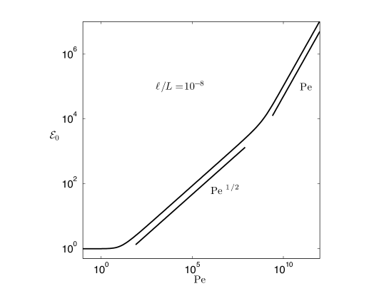
Figure 1: ${\cal E}_{0}$ as a function of $\mathrm{Pe}$ for cutoff source-sink distributions, after DoeringThiffeault2006 .

The scalings for the mixing efficiencies with a $\delta$-function source are apparently not all realized by a simple uniform wind as was the case for smooth monochromatic sources. We have performed the adiabatic approximation for the bulk variance in the case of a uniform wind blowing past a $\delta$-function source to estimate the mixing efficiencies (see Appendix B). While ${\cal E}_{1}$ is necessarily equal to 1 in both $2$-$d$ and $3$-$d$, we find that the uniform wind gives ${\cal E}_{0}\sim\sqrt{\mathrm{Pe}}$ (rather than the bound $\mathrm{Pe}/\sqrt{\log{\mathrm{Pe}}}$) in $2$-$d$, and ${\cal E}_{0}\sim\sqrt{\mathrm{Pe}}/\sqrt{\log{\mathrm{Pe}}}$ (significantly closer to the bound $\sqrt{\mathrm{Pe}}$) in $3$-$d$. For the large-scale efficiency, however, the uniform wind produces ${\cal E}_{-1}\sim\sqrt{\mathrm{Pe}}$ in both $2$-$d$ and $3$-$d$, far below its classically scaling upper bound.

A similar integral analysis can be carried out for “fractal” source-sink distributions where $|\hat{s}_{\bm{k}}|\sim|\bm{k}|^{-\gamma}$ with $\gamma\geq 0$. The scalings of the mixing efficiency bounds are summarized in Table 1. For $\gamma>d/2$ all the bounds scale classically since then $s(\bm{x})\in L^{2}(\mathbb{T}^{d})$. The case $\gamma=0$ is the $\delta$-function studied above. We observe that the bounds for ${\cal E}_{1}$ and ${\cal E}_{0}$ can exhibit anomalous scaling with exponents depending on the fractal nature of the source-sink distribution as characterized by $\gamma$ DoeringThiffeault2006 . Of course if the fractal scaling of the source-sink distribution persists over a broad but finite range of wavenumbers, say for $2\pi/L<k<2\pi/\ell_{s}$, then classical scaling for the efficiency estimates will again appear for $\mathrm{Pe}\gg L/\ell_{s}$.

Table 1: Scalings of the bound on the mixing efficiency ${\cal E}_{p}$ as functions of the source roughness exponent $\gamma$ of the source in two and three dimensions.

$d=2$	${p}=1$	${p}=0$	${p}=-1$
$\gamma=0$	1	$\rm{Pe}/(\log\rm{Pe})^{1/2}$	Pe
$0<\gamma<1$	$\rm{Pe}^{\gamma}$	Pe	Pe
$\gamma=1$	$\rm{Pe}/(\log\rm{Pe})^{1/2}$	Pe	Pe
$\gamma>1$	Pe	Pe	Pe
$d=3$
$\gamma=0$	1	$\rm{Pe}^{1/2}$	Pe
$0<\gamma<1/2$	1	$\rm{Pe}^{\gamma+1/2}$	Pe
$\gamma=1/2$	1	$\rm{Pe}/(\log{\rm{Pe}})^{1/2}$	Pe
$1/2<\gamma<3/2$	$\rm{Pe}^{\gamma-1/2}$	Pe	Pe
$\gamma=3/2$	$\rm{Pe}/(\log{\rm{Pe}})^{1/2}$	Pe	Pe
$\gamma>3/2$	Pe	Pe	Pe

VI A Single-scale Source Stirred by a Single-scale Flow

In the previous sections we have seen that the classical high-Péclet number scalings for the multi-scale mixing efficiencies, ${\cal E}_{p}\sim\mathrm{Pe}$, are generally upper bounds that may in fact be saturated for particular source-sink distributions stirred by certain statistically homogeneous and isotropic flows. It was shown in Section V that for some distribution-valued sources and sinks, some of the mixing efficiencies necessarily scale anomalously, i.e., ${\cal E}_{p}\lesssim\mathrm{Pe}^{\alpha_{p}}$ with some $\alpha_{p}<1$. For those examples the bounds on the mixing efficiencies at the different scales scale differently: $0\leq\alpha_{1}<\alpha_{0}<\alpha_{-1}=1$. It is not presently known if the anomalously scaling bounds for distribution-valued sources and sinks are sharp or, if they are, what kinds of statistically homogeneous and isotropic flows might be required to realize them. Those questions remain open, but in this section we settle the issue of the possibility of realizing distinct scaling exponents for the mixing efficiencies on different length scales for a smooth source-sink distribution.

The random sine flow, a.k.a. the renewing wave flow characterized by a single length scale, is a popular and convenient test bed for studying—both analytically and via simulation—a wide variety of stirring and mixing phenomena Pierrehumbert1994 ; Antonsen1996 ; Thiffeault2004 ; Tsang2005 . Here we consider the simplest single-scale source

$$s(\bm{x})=\sqrt{2}\,S\sin[2\pi(x+y)/L]$$ (VI.1)

stirred by a random sine flow that switches between

$$\bm{u}(\bm{x})=\hat{\bm{i}}\sqrt{2}\,U\sin[2\pi y/L+\phi]$$ (VI.2)

and

$$\bm{u}(\bm{x})=\hat{\bm{j}}\sqrt{2}\,U\sin[2\pi x/L+\phi]$$ (VI.3)

at time intervals of length $\tau/2$, where the phase $\phi$ is chosen randomly and uniformly from $[0,2\pi)$ at each switch. This is a statistically homogeneous and isotropic flow, but it is not the maximally efficient flow for this source-sink distribution; the optimal flow is the spatially uniform flow constructed in Section IV. We have performed high resolution direct numerical simulations of this system in $d=2$ spatial dimensions that reveal that the multi-scale mixing efficiencies may have distinct scaling exponents. Additionally, for this example we are able to compute the exponents theoretically in the context of the adiabatic averaging approximation utilized in Section IV.

Figure 2 shows the results of the direct numerical simulation for $p=1,0,-1$, each plotted along with the classically-scaling upper bounds from Section III. The Péclet number in these simulations was varied by holding $U=1$ fixed in a box of side length $L=1$ and changing the molecular diffusivity $\kappa$. The computations were carried out with switching time $\tau=1$. The details of the numerical simulations can be found in Thiffeault2004 .

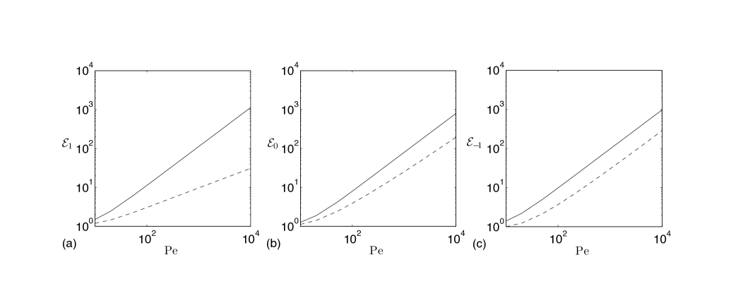
Figure 2: Mixing efficiencies ${\cal E}_{p}$ as a function of $\mathrm{Pe}$ for (a) $p=1$, (b) $p=0$, and (c) $p=-1$ for the random sine flow with source $\sim\sin k_{s}(x+y)$. The solid lines are the upper bounds for this source from Section III and the dashed lines are the data from the direct numerical simulations with $U$, $L$ and $\tau$ fixed.

Writing ${\cal E}_{p}\sim\mathrm{Pe}^{\alpha_{p}}$ as $\mathrm{Pe}\rightarrow\infty$, it is clear that the data are consistent with $\alpha_{0}<\alpha_{1}<1$ and $\alpha_{-1}\approx 1$.

These simulations establish two important facts: (1) that the mixing efficiencies at different length scales generally scale differently at high Péclet numbers, and (2) that anomalous subclassical scaling can easily be realized by simple and “reasonable” flows.

We can evaluate the observed scaling exponents $\alpha_{p}$ theoretically for this particular system by appealing to a quasi-static adiabatic approximation introduced in Section IV for the optimally mixing uniform flow. That is, we solve the time-independent problem for the scalar distribution under the influence of steady flows of the form (VI.2) and (VI.3), compute the variances, and average over the flow configurations. The physical justification for this approximation comes from examining the results of the direct numerical simulations: it is observed that the relevant steady-state configuration is quickly approached in the time intervals between the switches of the stirring field. If we make the switches at longer and longer intervals, i.e., if we increase $\tau$, the scalar field is distributed (nearly) according to the static configurations for most of the time, and the steady-state variances dominates the time averages.

The simplest problem in this category is when the velocity field is oriented parallel to the gradient of the source, so we consider the steady advection–diffusion equation

$$\sqrt{2}U\sin k_{u}y\ \partial_{x}\theta=\kappa(\partial_{x}^{2}+\partial_{y}^{2})\theta+\sqrt{2}S\sin k_{s}x$$ (VI.4)

where we allow for different length scales in the stirring and the source with the non-dimensional number $r=k_{u}/k_{s}$ gauging the relative amount of shear in the flow. This is not exactly the static problem corresponding to the dynamic simulations where the flow is always at a $45^{\circ}$ angle from the source-sink alignment, but it turns out that the scaling exponents $\alpha_{p}$ are the same for that case and for the $90^{\circ}$ alignment in (VI.4). For illustrative purposes it is convenient to explain the most elementary case (VI.4) in detail here and relegate details of the $45^{\circ}$ problem to Appendix C.

The solution to (VI.4) takes the form

$$\theta(\bm{x})=f(y)\sin(k_{s}x)+g(y)\cos(k_{s}x)$$ (VI.5)

where the functions $f$ and $g$ are periodic on $y\in[-\pi/k_{u},\pi/k_{u}]$ and satisfy the system of ODEs

$$-\sqrt{2}Uk_{s}\sin(k_{u}y)\,g(y) =\kappa\left[-k_{s}^{2}+\frac{d^{2}}{dy^{2}}\right]f(y)+\sqrt{2}S\,,$$ (VI.6a)

$$\sqrt{2}Uk_{s}\sin(k_{u}y)f(y) =\kappa\left[-k_{s}^{2}+\frac{d^{2}}{dy^{2}}\right]g(y)\,.$$ (VI.6b)

From (VI.6a) we deduce that $g(y)$ is an odd function of $y$ and $f(y)$ is an even function of $y$, compatible with (VI.6b) which says that $f$ and $g$ have opposite parity. We can thus infer boundary conditions on the reduced domain $[0,\pi/k_{u}]$:

$$g(0)=0=g(\pi/k_{u}),\quad f^{\prime}(0)=0=f^{\prime}(\pi/k_{u}).$$ (VI.7)

We are interested in the high-$\mathrm{Pe}$ behavior of the solution to (VI.4). In Figure 3 we show a grayscale plot of the scalar field at several values of the Péclet number. As is evident, internal layers develop along the lines of maximum shear around $y=n\pi/k_{u}$ for $n=0,\pm 1,\pm 2,\dots$. Away from these lines the flow directly blows source regions onto sink regions and vice versa which, as we have seen in Section IV, is the most efficient stirring to reduce variance at all scales. Even though the regions of high shear effectively stretch material lines, the mixing process is apparently frustrated by the constant replishment of the scalar variation by the steady sources and sinks and the variance is dominated by fluctuations concentrated in shear layers.

Figure 3: The scalar field stirred by a steady sine flow for (a) $\mathrm{Pe}$ = 0, (b) $\mathrm{Pe}$ = 100, (c) $\mathrm{Pe}$ = 1000.

We develop an asymptotic singular perturbation internal layer approach for the limit $\mathrm{Pe}\gg 1$ with $r={\cal O}(1)$ fixed. Upon rescaling $\tilde{y}=k_{s}y$, $\hat{f}=fUk_{s}/S$, $\hat{g}=gUk_{s}/S$, $r=k_{u}/k_{s}$, and introducing the slightly re-scaled Péclet number ${{\mathcal{P}}e}=\sqrt{2}U/\kappa k_{s}=\sqrt{2}\mathrm{Pe}/k_{s}L$ in Eqs. (VI.6), we obtain the non-dimensional ODEs

$$\frac{1}{{{\mathcal{P}}e}}\left[-1+\frac{d^{2}}{d\tilde{y}^{2}}\right]\hat{f}(\tilde{y})+1 =-\sin(r\tilde{y})\hat{g}(\tilde{y}),$$ (VI.8a)

$$\frac{1}{{{\mathcal{P}}e}}\left[-1+\frac{d^{2}}{d\tilde{y}^{2}}\right]\hat{g}(\tilde{y}) =\sin(r\tilde{y})\hat{f}(\tilde{y}).$$ (VI.8b)

Proceeding as usual we construct inner and outer solutions. The outer solution, valid away from the internal layers, is obtained by expanding in powers of ${{\mathcal{P}}e}^{-1}$:

$$\hat{f}_{\mathrm{outer}}=\sum_{n=0}^{\infty}{{\mathcal{P}}e}^{-n}\hat{f}_{n},\qquad\hat{g}_{\mathrm{outer}}=\sum_{n=0}^{\infty}{{\mathcal{P}}e}^{-n}\hat{g}_{n}.$$ (VI.9)

To leading order the solution to (VI.8) in the outer region is

$$\hat{f}_{\mathrm{outer}}\sim 0,\qquad\hat{g}_{\mathrm{outer}}\sim-\frac{1}{\sin(r\tilde{y})}\,.$$ (VI.10)

For the internal layer we expand in a small parameter $\epsilon$ as

$$\hat{f}_{\mathrm{inner}}=\sum_{n=-1}^{\infty}\epsilon^{n}\hat{f}_{n},\qquad\hat{g}_{\mathrm{inner}}=\sum_{n=-1}^{\infty}\epsilon^{n}\hat{g}_{n}\,,$$ (VI.11)

so that both $\hat{f}_{\mathrm{inner}}$ and $\hat{g}_{\mathrm{inner}}$ are ${\cal O}(\epsilon^{-1})$ as $\epsilon\rightarrow 0$. The internal layer scaling is determined by a dominant balance argument: we choose $\epsilon={{\mathcal{P}}e}^{-1/3}$ and rescale $\tilde{y}=\epsilon\,\eta$ to achieve a self-consistent scaling of the leading order terms. When these scalings and (VI.11) are inserted into (VI.8), the problem to solve at leading order ${\cal{O}}(1/\epsilon)$ is

$$\frac{d^{2}\hat{f}_{-1}}{d\eta^{2}}+r\eta\hat{g}_{-1}+1=0,\qquad\frac{d^{2}\hat{g}_{-1}}{d\eta^{2}}-r\eta\hat{f}_{-1}=0.$$ (VI.12)

Then letting $\xi=r^{1/3}\eta$, $F=r^{2/3}\hat{f}_{-1}$, and $G=r^{2/3}\hat{g}_{-1}$, (VI.12) simplifies to the inner layer equations

$$F^{{}^{\prime\prime}}+\xi G+1=0,\qquad G^{{}^{\prime\prime}}-\xi F=0,$$ (VI.13)

with boundary conditions $F^{\prime}(0)=0$ and $G(0)=0$. The other boundary conditions come from the requirement of matching to the outer solution (VI.10): $F(\xi)\rightarrow 0$ and $G(\xi)\rightarrow-1/\xi$ as $\xi\rightarrow\infty$. The system (VI.13) can be cast as a complex Airy equation for $F+iG$, but we resort instead to a numerical shooting method to obtain the solution.

The solution of the internal layer equations is obtained by shooting backward (which is the more stable evolution direction) from $\xi\rightarrow\infty$. The large-$\xi$ asymptotic behavior deduced from (VI.13) is

$$F\approx-\frac{2}{\xi^{4}}+\frac{a}{\xi^{10}}\,,\qquad G\approx-\frac{1}{\xi}+\frac{b}{\xi^{7}}\,,$$ (VI.14)

where in practice $a$ and $b$ are tuned numerically to produce a solution that satisfies the boundary conditions at $\xi=0$. This is easily accomplished, and in Figure 4 we compare the internal layer solution against the exact (numerical) solution of the full advection–diffusion equation (VI.4) at $\mathrm{Pe}=1000$ where the small parameter $\epsilon\approx.2$. This agreement confirms that the leading terms

$$\hat{f}_{\mathrm{inner}}=\frac{r^{-2/3}}{\epsilon}\,F(\xi),\qquad\hat{g}_{\mathrm{inner}}=\frac{r^{-2/3}}{\epsilon}\,G(\xi).$$ (VI.15)

do indeed accurately capture the asymptotic behavior.

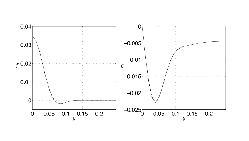
Figure 4: Comparison of the direct numerical solution (solid) and the internal layer solution (dashed) for $\mathrm{Pe}$ = 1000.

The uniform asymptotic solution to the coupled ODEs are, to leading order, the composites of the inner and outer solutions. Recovering all the scalings and letting $\delta=\epsilon/r^{1/3}k_{s}$, we define

$$f_{\mathrm{comp}}(y)\ =\ \frac{S}{Uk_{s}}\,\hat{f}_{\mathrm{inner}}(y)\ =\frac{S}{Uk_{s}}\,\frac{1}{k_{u}\delta}F\left(\frac{y}{\delta}\right),$$ (VI.16a)

$$g_{\mathrm{comp}}(y)\ =\ \frac{S}{Uk_{s}}\,k_{u}y\times\hat{g}_{\mathrm{inner}}(y)\times\hat{g}_{\mathrm{outer}}(y)\ =\frac{S}{Uk_{s}}\,\frac{1}{k_{u}\delta}\,\frac{k_{u}y}{\sin(k_{u}y)}\,G\left(\frac{y}{\delta}\right).$$ (VI.16b)

Armed with the approximate solutions (VI.16) we can compute the multi-scale mixing measures $\langle|\nabla^{p}\theta|^{2}\rangle$ for $p=0,1,-1$.

The variance is

$$\langle\theta^{2}\rangle=\frac{1}{2}\left(\langle f^{2}\rangle+\langle g^{2}\rangle\right)=\frac{1}{2}\frac{4k_{u}}{\pi}\left(\int_{0}^{\pi/4k_{u}}f(y)^{2}dy+\int_{0}^{\pi/4k_{u}}g(y)^{2}dy\right)$$ (VI.17)

where we use the symmetry of the solution to carry out the integral over only a quarter-period. Letting $\eta=y/\delta$ and replacing $f$ and $g$ by $f_{\mathrm{comp}}$ and $g_{\mathrm{comp}}$,

$$\langle\theta^{2}\rangle\ \sim\ \frac{1}{\pi}\frac{S^{2}}{U^{2}k_{s}^{2}}\frac{1}{k_{u}\delta}\left(\int_{0}^{\pi/2k_{u}\delta}F(\eta)^{2}d\eta+\int_{0}^{\pi/2k_{u}\delta}G(\eta)^{2}\frac{k_{u}^{2}\eta^{2}\delta^{2}}{\sin^{2}(k_{u}\eta\delta)}d\eta\right).$$ (VI.18)

Here we are interested in the scaling as $\delta\rightarrow 0$ so we are justified in replacing the upper limit of the integral of $F(\eta)^{2}$ by infinity. Slightly more care must be taken with the integral involving $G(\eta)^{2}$: because $k_{u}^{2}\eta^{2}\delta^{2}/\sin^{2}(k_{u}\eta\delta)$ is uniformly bounded by $0$ and $\pi/2$ we can appeal to Lebesgue’s dominated convergence theorem to deduce

$$\langle\theta^{2}\rangle\ \sim\ \frac{1}{\pi}\frac{S^{2}}{U^{2}k_{s}^{2}}\frac{1}{k_{u}\delta}\left(\int_{0}^{\infty}F(\eta)^{2}d\eta+\int_{0}^{\infty}G(\eta)^{2}d\eta\right).$$ (VI.19)

The unstirred variance is $\langle\theta_{0}^{2}\rangle=S^{2}/\kappa^{2}k_{s}^{4}$, so the mixing efficiency is

$${\cal E}_{0}\ \sim\ \sqrt{\frac{\pi}{2}}\,\left(\int_{0}^{\infty}F(\eta)^{2}d\eta+\int_{0}^{\infty}G(\eta)^{2}d\eta\right)^{-1/2}\,r^{1/3}\,{{\mathcal{P}}e}^{5/6}.$$ (VI.20)

Figure 5 shows ${\cal E}_{0}$ as a function of $\mathrm{Pe}$ from the numerical solution of the steady advection–diffusion equation (VI.4). The data accurately match the $\mathrm{Pe}^{5/6}$ scaling and using the prefactor calculated from (VI.20) there is only a 5% discrepancy between the internal layer solution and that calculated from the direct numerical simulation at $\mathrm{Pe}=1000$ with $r=1$. Remarkably, this $\mathrm{Pe}^{5/6}$ scaling also fits the data for the time-dependent stirring of the tilted source shown in Figure 2.

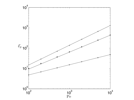
Figure 5: Mixing efficiencies ${\cal E}_{p}$ for $p=1$ (x), $p=0$ (*) and $p=-1$ (+) for the steady sine flow. The solid lines are the scaling predictions of the asymptotic analysis and the discrete data are from the numerical solution of the steady advection–diffusion equation (VI.4).

The gradient variance in the steady solution is given by

$$\langle|\nabla\theta|^{2}\big{\rangle}=\frac{k_{s}^{2}}{2}\left[\langle f^{2}\rangle+\langle g^{2}\rangle\right]+\frac{1}{2}\left[\langle(f^{\prime})^{2}\rangle+\langle(g^{\prime})^{2}\rangle\right].$$ (VI.21)

The $\langle f^{2}\rangle$ and $\langle g^{2}\rangle$ terms were computed above in the context of ${\cal E}_{0}$, so we focus on the derivative terms. Inserting the composite asymptotic solution (VI.16) we obtain

$$\frac{1}{2}\left[\langle(f^{\prime})^{2}\rangle+\langle(g^{\prime})^{2}\rangle\right]\sim\left\langle\left(\frac{S}{Uk_{s}}\frac{1}{k_{u}\delta^{2}}F^{\prime}(y/\delta)\right)^{2}\right\rangle+\\ \left\langle\left(\frac{S}{Uk_{s}}\frac{1}{k_{u}\delta^{2}}G^{\prime}(y/\delta)\frac{k_{u}y}{\sin(py)}+\frac{S}{Uk_{s}}\frac{1}{k_{u}\delta}G(y/\delta)\left[\frac{k_{u}y}{\sin(k_{u}y)}\right]^{\prime}\right)^{2}\right\rangle.$$

The last term is smaller (${\cal O}(\delta^{-1})$) than the immediately preceeding term (${\cal O}(\delta^{-2})$) and may thus be neglected. The first two terms in (VI.21) are also ${\cal O}(\delta^{-1})$, so they may be neglected as well. Hence

$$\frac{1}{2}\left[\langle(f^{\prime})^{2}\rangle+\langle(g^{\prime})^{2}\rangle\right]\sim\frac{1}{\pi}\frac{S^{2}}{U^{2}k_{s}^{2}}\frac{1}{k_{u}\delta^{3}}\left[\int^{\pi/2k_{u}\delta}_{0}F^{\prime}(\eta)^{2}d\eta+\int^{\pi/2k_{u}\delta}_{0}G^{\prime}(\eta)^{2}\frac{k_{u}^{2}\eta^{2}\delta^{2}}{\sin^{2}(k_{u}\eta\delta)}d\eta\right]$$

and by the same arguments as for the variance above we deduce

$$\langle|\nabla\theta|^{2}\big{\rangle}\sim\frac{1}{\pi}\left(\int_{0}^{\infty}F^{\prime}(\eta)^{2}d\eta+\int_{0}^{\infty}G^{\prime}(\eta)^{2}d\eta\right)\frac{S^{2}}{U^{2}k_{s}^{2}}\frac{1}{k_{u}\delta^{3}}\,.$$ (VI.22)

Using $\langle|\nabla\theta_{0}|^{2}\rangle=S^{2}/\kappa^{2}k_{s}^{2}$, we deduce that the mixing efficiency is

$${\cal E}_{1}\ \sim\ \sqrt{\frac{\pi}{2}}\,\left(\int_{0}^{\infty}F^{\prime}(\eta)^{2}d\eta+\int_{0}^{\infty}G^{\prime}(\eta)^{2}d\eta\right)^{-1/2}\,{{\mathcal{P}}e}^{1/2}.$$ (VI.23)

Figure 5 also shows the scaling of ${\cal E}_{1}$ from the numerical solution of (VI.4). The internal layer asymptotic approximation in (VI.23) and the numerical solutions differ by approximately 1% at $\mathrm{Pe}$ = 1000. The (lack of) scaling in $r$ was also confirmed numerically. Interestingly, for this problem stirring at ever smaller scales does not further enhance the mixing efficiency on small scales. This is apparently because the decrease in gradient variance due to stirring on small scales is compensated by the increase in gradient variance in the internal layer.

The inverse-gradient variance,

$$\langle|\nabla^{-1}\theta|^{2}\rangle\ =\ \langle|\nabla^{-1}(f(y)\sin(k_{s}x)+g(y)\cos(k_{s}x))|^{2}\rangle,$$ (VI.24)

requires a slightly more subtle analysis. Expanding $f(y)$ and $g(y)$ in Fourier series,

$$f(y)=\sum_{n=0}^{\infty}f_{n}\cos(nk_{u}y),\quad\quad g(y)=\sum_{n=1}^{\infty}g_{n}\sin(nk_{u}y)$$ (VI.25)

the inverse gradient variance is

$$\langle|\nabla^{-1}\theta|^{2}\rangle\ =\ \frac{f_{0}^{2}}{2k_{s}^{2}}+\frac{1}{4}\sum_{n=1}^{\infty}\frac{f_{n}^{2}+g_{n}^{2}}{k_{s}^{2}+n^{2}k_{u}^{2}}.$$ (VI.26)

We know that ${\cal E}_{-1}\lesssim\mathrm{Pe}$, so if we could establish a lower bound with the same scaling then we could conclude that ${\cal E}_{-1}$ scales classically $\sim\mathrm{Pe}$. Hence we focus on deducing an asymptotic upper bound on $\langle|\nabla^{-1}\theta|^{2}\rangle$. As will be seen, however, the best we can do is assert the classical scaling with a logarithmic correction.

Toward that end, using the fact that $\sum_{n=1}^{\infty}n^{-2}=\pi^{2}/6$,

$$\langle|\nabla^{-1}\theta|^{2}\rangle\ \leq\ \frac{f_{0}^{2}}{2k_{s}^{2}}\ +\ \frac{\pi^{2}}{24k_{u}^{2}}\,\sup_{n\geq 1}(f_{n}^{2}+g_{n}^{2}).$$ (VI.27)

Then the key is to note that the Fourier coefficients $f_{n}$ are all ${\cal O}(S/Uk_{s})$—without any further factors of $\delta$ appearing—while the $g_{n}$ are ${\cal O}(S/Uk_{s}\times\log{\frac{1}{\delta}})$. Indeed,

$$|f_{n}|\ =\ \left|\frac{(2-\delta_{n,0})k_{u}}{\pi}\int_{-\pi/2k_{u}}^{\pi/2k_{u}}f(y)\cos(nk_{u}y)dy\,\right|\ \lesssim\ \frac{2(2-\delta_{n,0})S}{\pi Uk_{s}}\int_{0}^{\infty}|F(\eta)|\,d\eta$$ (VI.28)

while

$$|g_{n}|\ = \left|\frac{2k_{u}}{\pi}\int_{-\pi/2k_{u}}^{\pi/2k_{u}}g(y)\sin(nk_{u}y)dy\,\right|$$ (VI.29)

$$\sim \frac{2S}{\pi Uk_{s}}\left|\int_{-\pi/2k_{u}\delta}^{\pi/2k_{u}\delta}\frac{k_{u}\delta\,\eta}{\sin(k_{u}\delta\,\eta)}G(\eta)\sin(nk_{u}\delta\,\eta)d\eta\,\right|$$

$$\leq \frac{2S}{Uk_{s}}\int_{0}^{\pi/2k_{u}\delta}|G(\eta)|\,d\eta\,\ \sim\ \frac{2S}{Uk_{s}}\log\left[\frac{1}{k_{u}\delta}\right].$$

In the last step above we used the fact that $|G(\eta)|\sim\eta^{-1}$ as $\eta\rightarrow\infty$.

The unstirred large-scale variance is $\langle|\nabla^{-1}\theta_{0}|^{2}\rangle=S^{2}/\kappa^{2}k_{s}^{6}$, so we deduce the large-scale mixing efficiency obeys

$${\cal E}_{-1}\ \geq\ C\,\frac{\mathrm{Pe}}{k_{s}L}\times\frac{1}{\sqrt{{1+C^{\prime}\left(\frac{\log{\mathrm{Pe}}}{r}\right)^{2}}}}$$ (VI.30)

where $C$ and $C^{\prime}$ are absolute constants. The numerical solutions of the steady advection–diffusion equation shown in Figure 5 confirms this classical scaling; the logarithmic term is not visible for this range of $\mathrm{Pe}$. Again, this is consistent with the dynamic data for ${\cal E}_{-1}$ in Figure 2.

VII Summary and Discussion

The suppression of bulk variance of a scalar field is a natural gauge of the efficiency of stirring, and this notion allows for the examination of the effect of a flow on various length scales. We have quantified the influence of stirring on weighted bulk variances in terms of nondimensional mixing efficiencies ${\cal E}_{p}$ that characterize fluctuations on relatively small ($p=1$), intermediate ($p=0$) and large ($p=-1$) length scales. We studied these mixing efficiencies for statistically stationary, homogeneous and isotropic flow fields stirring scalars sustained by a variety of steady but spatially inhomogeneous scalar sources and sinks on periodic domains. We reach a number of conclusions:

• Very generally, the mixing efficiencies ${\cal E}_{p}$ are bounded from below $\sim\mathrm{Pe}^{0}$ at high Péclet numbers—indicating ineffective stirring—and from above $\sim\mathrm{Pe}^{1}$—the classical scaling anticipated by the simplest eddy diffusion theory. Classical scaling of the efficiencies corresponds to the existence of residual supression of variance in the vanishing diffusion ($\kappa\rightarrow 0$) limit.

• Source, sink and statistically stationary homogeneous and isotropic flow combinations exist that realize both the upper and lower bounds’ scaling with respect to $\mathrm{Pe}$—and in some cases the prefactors as well—showing that the analysis is sharp at the most general level.

• The small and intermediate scale mixing efficiencies ${\cal E}_{1}$ and ${\cal E}_{0}$ are ultimately limited by length scales in the source-sink distributions. That is, even if the efficiencies scale classically the inferred mixing lengths $\sim\kappa\mathrm{Pe}/U$ are limited by length scales defined by the sources and sinks rather than by the spectrum of scales in the flow. On the other hand the upper bound analysis does not prevent small scales in the flow field from enhancing suppression of the variance at large scales, i.e., ${\cal E}_{-1}$, to an unlimited degree.

• Sufficiently “rough” scalar sources and sinks, in particular non-square-integrable distributions, necessarily produce sub-classical scaling of ${\cal E}_{0}$ and/or ${\cal E}_{1}$ at high Péclet numbers. In such cases there is no residual suppression of variance in the vanishing diffusion limit for any finite mean kinetic energy statistically stationary homogeneous and isotropic stirring.

• The mixing efficiencies at various length scales need not scale the same as $\mathrm{Pe}\rightarrow\infty$. This was illustrated explicitly by the example of a monochromatic source distribution stirred by the random sine flow. We found by direct numerical simulation and an adiabatic asymptotic internal layer analysis that for small scales ${\cal E}_{1}\sim\mathrm{Pe}^{1/2}$, for intermediate scales ${\cal E}_{0}\sim\mathrm{Pe}^{5/6}$, and the large length scale efficiency ${\cal E}_{-1}$ exhibits near-classical scaling $\sim\mathrm{Pe}/\log{\mathrm{Pe}}$.

The analysis, simulations and modeling presented in this paper have addressed some fundamental questions regarding suppression of the long time averaged bulk scalar variance via stirring by incompressible and statistically homogeneous and isotropic flow fields, but compelling challenges remain for future study. Among the unsolved problems open questions are:

• Can the anomalous mixing efficiency bounds for measure-valued or fractal sources be achieved by any statistically stationary homogeneous and isotropic flow? This is a difficult problem for direct numerical simulations of the advection–diffusion equation because of the small spatial scales that need to be resolved. An alternate simulation approach is particle tracking, by following the evolution of many discrete particles moving with the flow and diffusing and approximating the continuous scalar concentration on an appropriately coarse grained level.

• Can the small-flow-scale enhancement of the large-scale mixing efficiency ${\cal E}_{-1}$, as suggested by the upper bound in (III.43), be realized? It makes sense that stirring may be capable of suppressing large-scale variance, even for negligible molecular diffusion, by transferring scalar inhomogeneities from large length scales to small length scales via kinetic stretching and folding mechanisms. The upper bound provides a quantitative estimate of this effect and it will be interesting to see to what extent it is an accurate estimate.

• What is the mixing efficiency of “real” stationary homogeneous and isotropic turbulence in two and three dimensions? The bounds derived here all apply to these flows, and the inevitable limitations on the mixing efficiency imposed by the source and sink structure apply. Turbulent mixing by a fluid with viscosity $\nu$ is often characterized by a Reynolds number $\text{Re}=UL/\nu$ and a Schmidt number $\text{Sc}=\nu/\kappa$. While the mixing efficiencies ${\cal E}_{p}$ are studied here as functions of $\mathrm{Pe}=\text{Re}\times\text{Sc}$, the separate Reynolds and Schmidt number dependences are of interest, too. These questions can be investigated theoretically and via direct numerical simulations in the periodic domain setting utilized here.

• The uniform-wind optimal solution presented in Section IV is only appropriate for a one-dimensional source distribution in a domain with periodic boundary conditions. It is optimal by virtue of always having a component blowing along the source gradient, so no time and little energy is wasted blowing along lines of constant source. If the source has a more complicated structure, then it is not generally possible to achieve such an efficient flow while preserving incompressibility. Physical boundaries or a different golbal topology (e.g. a spherical domain as relevant to geophysical applications) will likewise invalidate the uniform-wind solution. The general question is then: For a given distribution of sources and sinks in a given domain, what is the optimal stirring strategy to achieve the greatest reduction of bulk variance? This question has obvious relevance to engineering applications. While we have answered it in the simplest setting of a single mode source-sink distribution on a periodic domain, it is clearly a complex problem in general. It is not unlikely, however, that intuition gained from the study of idealized models may contribute to the development of valuable intuition for such systems.

• Bounded domains with rigid walls are more appropriate for some engineering applications. Then the scalar sources and/or sinks can be implemented by boundary conditions rather than as body sources and sinks Balmforth2003 . We can also imagine situations where fluid and/or imposed scalar fluxes at boundaries contribute to the scalar variance in the bulk. How this will affect the efficiency scalings is an open question.

• We have seen that very generally ${\cal E}_{1}\geq 1$, but have only established a similar lower bound on ${\cal E}_{0}$ and ${\cal E}_{-1}$ for the simplest case of monchromatic sources. It is an open question whether or not there exist source, sink and flow (even steady flow) combinations where ${\cal E}_{0}$ and/or ${\cal E}_{-1}<1$. It is worthwhile noting in this context that in all cases $\langle\theta^{2}\rangle^{2}\leq\langle|\nabla\theta|^{2}\rangle\langle|\nabla^{-1}\theta|^{2}\rangle$. Any stirring decreases the mean bulk gradient variance, but this suggests that if it does not decrease the variance significantly then it would have to increase the inverse gradient variance. Hence it may not be surprising to find flows that can amplify large-scale fluctuations.

• A related problem of interest is the advection–diffusion of a passive scalar $\theta$ with decay rate $\zeta$ sustained by a body source with evolution described by

  $$\frac{\partial\theta}{\partial t}+\bm{u}\cdot\nabla\theta=\kappa\Delta\theta+s(\bm{x})-\zeta\theta.$$ (VII.1)

  In applications $\zeta$ may have an interpretation as a chemical reaction rate or a radiative relaxation rate relevant in meteorology or for other geophysical flows on the sphere. A linear amplitude damping term in the advection–diffusion equation introduces new features such as competition between scalar decay and mixing to supress steady-state variances ShawGFD2005 .

• Finally, all the questions above can be posed for time dependent sources and sinks.

Appendix A Lower Bound on Variance Efficiency

One might expect the variance efficiency ${\cal E}_{0}$ to have a lower bound of unity, implying that stirring always decreases the variance. In order to derive a uniform (in $\mathrm{Pe}$) lower estimate we can search for the maximum variance subject to the steady-state production-dissipation constraint:

$$\langle\theta^{2}\rangle\geq\min_{\vartheta}~{}\{\langle\vartheta^{2}\rangle~{}|~{}\kappa\langle|\nabla\vartheta|^{2}\rangle=\langle s\vartheta\rangle\}.$$ (A.1)

The solution of this optimization problem in Fourier space is

$$\hat{\theta}(\bm{k})=\frac{\mu}{2}\frac{\hat{s}(\bm{k})}{\mu\kappa k^{2}+1}$$ (A.2)

where $\mu$ is the Lagrange multiplier enforcing the constraint

$$\kappa\sum_{\bm{k}}k^{2}|\hat{\theta}(\bm{k})|^{2}=\sum_{\bm{k}}\hat{\theta}(\bm{k})\hat{s}^{*}(\bm{k})~{}~{}\quad\Longrightarrow\quad\kappa\sum_{\bm{k}}\frac{\mu k^{2}|\hat{s}(\bm{k})|^{2}}{(\mu\kappa k^{2}+1)^{2}}=2\sum_{\bm{k}}\frac{|\hat{s}(\bm{k})|^{2}}{\mu\kappa k^{2}+1}.$$ (A.3)

where $*$ denotes the complex conjugate.

In the case of a dichromatic source with wavenumber $k_{1}$ at amplitude $s_{1}$ and $k_{2}$ at amplitude $s_{2}$, the constraint requires one to solve a cubic equation for $\xi=1/\mu\kappa k_{1}^{2}$,

$$(1+\alpha)\xi^{3}+\tfrac{1}{2}(1+\alpha\beta+4\beta+4\alpha)\xi^{2}+(\beta+\alpha\beta+\beta^{2}+\alpha)\xi+\tfrac{1}{2}(\beta^{2}+\alpha\beta)=0$$ (A.4)

where $\alpha=s_{1}^{2}/s_{2}^{2}$ and $\beta=k_{1}^{2}/k_{2}^{2}$. Then the mixing efficiency bound is

$${\cal E}_{0}^{2}\geq\frac{\sum_{k_{1},k_{2}}|\hat{\theta}_{0}(\bm{k})|^{2}}{\sum_{k_{1},k_{2}}|\hat{\theta}(\bm{k})|^{2}}=\frac{4(1+\frac{\alpha}{\beta^{2}})}{\frac{1}{(1+\xi)^{2}}+\frac{\alpha}{(\beta+\xi)^{2}}},$$ (A.5)

and a numerical evaluation of the roots reveals that the minimum value of the efficiency bound is less than 1 for $\forall~{}\xi$. Thus the variance production-dissipation balance alone does not rule out the existence of flows that could increase the scalar variance.

Appendix B Steady uniform wind on a $\delta$-function source

Taking the Fourier transform of the steady advection–diffusion equation (I.3) with a uniform velocity field along the $x_{d}$-axis,

$$\hat{\theta}(\bm{k})=\frac{\hat{s}(\bm{k})}{\kappa k^{2}+iUk_{d}}$$ (B.1)

where $k_{d}$ is the $d$th component of the horizontal wavenumber. Now substitute $\hat{s}(\bm{k})=\text{const}$ for a $\delta$-function source and after approximating the sums by integrals (since we are only interested in the asymptotic behavior), we find

$$d =2:\qquad \langle|\nabla^{p}\theta|^{2}\rangle =\int_{0}^{2\pi}d\phi\int_{2\pi/L}^{\infty}\frac{k^{2p+1}dk}{\kappa^{2}k^{4}+U^{2}k^{2}\cos^{2}\phi}\,,$$ (B.2a)

$$d =3: \langle|\nabla^{p}\theta|^{2}\rangle =\int_{0}^{2\pi}d\phi\int_{0}^{\pi}\sin\vartheta d\vartheta\int_{2\pi/L}^{\infty}\frac{k^{2(p+1)}dk}{\kappa^{2}k^{4}+U^{2}k^{2}\cos^{2}\vartheta}\,.$$ (B.2b)

The variances in the absence of stirring are found by calculating the integrals (B.2) with $U=0$. Straightforward evaluation of the integrals (B.2) yields

$$d =2:\qquad {\cal E}_{1} =1,\quad {\cal E}_{0} \sim\sqrt{\mathrm{Pe}}\,,\quad {\cal E}_{-1} \sim\sqrt{\mathrm{Pe}}\,,$$ (B.3a)

$$d =3: {\cal E}_{1} =1,\quad {\cal E}_{0} \sim\frac{\sqrt{\mathrm{Pe}}}{\sqrt{\log\mathrm{Pe}}}\,,\quad {\cal E}_{-1} \sim\sqrt{\mathrm{Pe}}\,.$$ (B.3b)

These anomalous scalings in $\mathrm{Pe}$ suggest that the uniform flow is not the optimal allowed by the bound for the $\delta$-function source in both $d=2$ and $3$. This emphasizes the source-dependent nature of the optimal stirrer.

Appendix C Steady shear at an angle

When the source is tilted at a 45^∘ angle, i.e. $s(\bm{x})=\sqrt{2}S\sin(k_{s}(x+y))$, the functions $f$ and $g$ must satisfy

$$-\sqrt{2}Uk_{s}\sin(k_{u}y)\,g(y) =\kappa\left[-k_{s}^{2}+\frac{d^{2}}{dy^{2}}\right]f(y)+\sqrt{2}S\sin(k_{s}y)\,,$$ (C.1a)

$$\sqrt{2}Uk_{s}\sin(k_{u}y)f(y) =\kappa\left[-k_{s}^{2}+\frac{d^{2}}{dy^{2}}\right]g(y)+\sqrt{2}S\cos(k_{s}y)\,.$$ (C.1b)

Upon changing variables as done in section $\rm{VII}$ we obtain

$$\frac{1}{{{\mathcal{P}}e}}\left[-1+\frac{d^{2}}{d\tilde{y}^{2}}\right]\hat{f}(\tilde{y})+\sin\tilde{y} =-\sin(r\tilde{y})\hat{g}(\tilde{y}),$$ (C.2a)

$$\frac{1}{{{\mathcal{P}}e}}\left[-1+\frac{d^{2}}{d\tilde{y}^{2}}\right]\hat{g}(\tilde{y})+\cos\tilde{y} =\sin(r\tilde{y})\hat{f}(\tilde{y}).$$ (C.2b)

The internal layer solution is once again obtained by expanding in powers of ${{\mathcal{P}}e}^{-1}$. To leading order the solution to (C.2) in the outer region is

$$\hat{f}_{\mathrm{outer}}\sim 1,\qquad\hat{g}_{\mathrm{outer}}\sim-\frac{1}{\tan(r\tilde{y})}\,.$$ (C.3)

The inner internal layer solution is the same as for the untilted source problem. In Figure 6 we compare the internal layer solution against the exact (numerical) solution of the full advection–diffusion equation (VI.4) at $\mathrm{Pe}=1000$ where the small parameter $\epsilon\approx.2$.

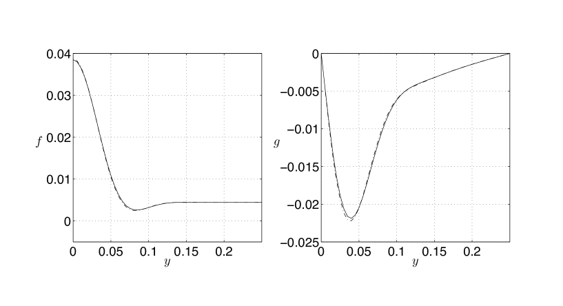
Figure 6: Comparison of the direct numerical solution (solid) and the internal layer solution (dashed) for $\mathrm{Pe}$ = 1000.

Recovering all the scalings and letting $\delta=\epsilon/r^{1/3}k_{s}$, we define the composite approximations

$$f_{\mathrm{comp}}(y)\ =\ \frac{S}{Uk_{s}}\,[\hat{f}_{\mathrm{inner}}(y)+f_{\mathrm{outer}}(y)]\ =\frac{S}{Uk_{s}}\,\left[\frac{1}{k_{u}\delta}F\left(\frac{y}{\delta}\right)+1\right],$$ (C.4a)

$$g_{\mathrm{comp}}(y)\ =\ \frac{S}{Uk_{s}}\,k_{u}y\times\hat{g}_{\mathrm{inner}}(y)\times\hat{g}_{\mathrm{outer}}(y)\ =\frac{S}{Uk_{s}}\,\frac{1}{k_{u}\delta}\,\frac{k_{u}y}{\tan(k_{u}y)}\,G\left(\frac{y}{\delta}\right).$$ (C.4b)

Given the internal layer solution we can compute the multi-scale mixing measures. In fact, to leading order the dependence of the efficiencies on the Péclet number is the same. The difference is in the prefactors. Figure 7 compares the scalings derived from the internal layer solution (including prefactors) to the discrete data from the numerical solution and the numerical solution using the random sine flow.

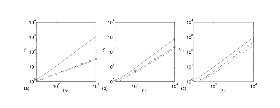
Figure 7: Mixing efficiencies ${\cal E}_{p}$ as a function of $\mathrm{Pe}$ for (a) $p=1$, (b) $p=0$, and (c) $p=-1$. The solid lines are the bounds, the dashed-dot lines are scalings predicted from the internal layer asymptotic analysis, the open circles are the discrete data from the numerical solution of the steady advection–diffusion equation (VI.4), and the dashed lines are the result of the direct numerical solution for the time-dependent random sine flow.

Appendix D Corrigendum (29 April 2011)

In this corrigendum we rectify an error in the published version of this preprint (Shaw et al. Shaw2007 ). In Section III.1 we obtained an estimate on the variance of the concentration $\theta(\bm{x})$ of an advected passive scalar. We did this by solving the optimization problem

$$\langle\theta^{2}\rangle\leq\max_{\vartheta}\,\{\langle\vartheta^{2}\rangle\,|\,\kappa\langle|\nabla\vartheta|^{2}\rangle=\langle s\vartheta\rangle\}$$ (D.1)

where the angle brackets denote spatial averaging, $\kappa$ is the diffusivity, and $s(\bm{x})$ is the spatially-dependent source with spatial mean zero. The constraint in (D.1) arises from integrating the advection-diffusion equation with periodic boundary conditions. The Euler–Lagrange equation for the extremizer $\vartheta_{*}(\bm{x})$ is

$$2\vartheta_{*}-2\mu\kappa\Delta\vartheta_{*}-\mu s=0$$ (D.2)

where $\mu$ is the Lagrange multiplier enforcing the constraint in (D.1). In terms of the Fourier coefficients the solution of (D.2) is straightforward:

$${\hat{\vartheta}_{*}}{}_{\bm{k}}=\tfrac{1}{2}{\mu}\,\frac{\hat{s}_{\bm{k}}}{\mu\kappa k^{2}+1},\qquad\sum_{{\bm{k}}}\frac{2+\mu\kappa k^{2}}{(\mu\kappa k^{2}+1)^{2}}\,|\hat{s}_{\bm{k}}|^{2}=0.$$ (D.3)

that latter being an equation for $\mu<0$. If the source is “monochromatic,” i.e., is an eigenmode of the Laplacian with eigenvalue $-k_{\mathrm{s}}^{2}$, then the solution (D.3) simplifies to

$$\mu^{\text{mono}}=-2/(\kappa k_{\mathrm{s}}^{2}),\qquad\vartheta_{*}^{\text{mono}}=s/(\kappa k_{\mathrm{s}}^{2})\qquad\text{(monochromatic source)}.$$ (D.4)

From (D.4) Shaw et al. inferred that for monochromatic sources the variance $\langle\theta^{2}\rangle$ could never decrease below its value in the absence of any stirring flow. That is, for monochromatic sources there are no ‘unmixing’ velocity fields which raise variance rather than lower it.

The problem with the solution (D.3) (and its monochromatic limit (D.4)) is that it is not always a maximum for (D.1). To see this, let $\theta=\vartheta_{*}+\delta\theta$. We have

$$\langle\theta^{2}\rangle=\langle\vartheta_{*}^{2}\rangle+F,\qquad F\mathrel{\raisebox{0.29707pt}{:}\!\!=}2\langle\vartheta_{*}\delta\theta\rangle+\langle(\delta\theta)^{2}\rangle,$$ (D.5)

so we want to investigate the sign of $F$ to determine if $\vartheta_{*}$ is indeed a maximum. After enforcing the constraint in (D.1) and integrating by parts we can derive

$$F=\mu\kappa\langle\lvert\nabla\delta\theta\rvert^{2}\rangle+\langle(\delta\theta)^{2}\rangle.$$ (D.6)

from which an application of Poincaré’s inequality gives

$$F\leq\mu\kappa\langle\lvert\nabla\delta\theta\rvert^{2}\rangle+K^{-2}\langle\lvert\nabla\delta\theta\rvert^{2}\rangle=\left(K^{-2}+\mu\kappa\right)\langle\lvert\nabla\delta\theta\rvert^{2}\rangle$$ (D.7)

where $K=2\pi/L$ is the smallest allowable wavenumber, with $L$ the size of the periodic domain. Thus, $F$ is guaranteed to be negative (and $\vartheta_{*}$ is a maximum) if

$$-\mu\kappa K^{2}\geq 1.$$ (D.8)

(Showing that this is true when equality holds in (D.8) requires a slightly longer analysis.) We can also show that if (D.8) is violated, then there are values of $\delta\theta$ that make $F$ negative, showing that (D.8) is necessary in addition to being sufficient.

For monochromatic sources, inserting (D.4) into (D.8) implies that we are guaranteed to have a maximum if

$$k_{\mathrm{s}}^{2}\leq 2K^{2}\qquad\text{(monochromatic source)}.$$ (D.9)

Larger values of $k_{\mathrm{s}}$ leave open the possibility of $\vartheta_{*}$ not being a maximum, and indeed this is the case, as shown in Thiffeault2011_review . Thus, it is not true as claimed in Shaw2007 that all monochromatic sources have $\langle\vartheta_{*}^{2}\rangle$ as a maximum variance: the only ones that do have small wavenumber $k_{\mathrm{s}}$ satisfying (D.9). In particular this means that many monochromatic sources can have mixing efficiency $\mathcal{E}_{0}$ less than unity (the same is true for $\mathcal{E}_{-1}$; see Shaw2007 for definitions).

We emphasize that we expect that generic velocity fields will decrease variance, and so will be ‘efficient’ stirrers. It is still an open question to characterize the sources that cannot lead to an increase in variance, that is, for which unmixing flows do not exist.

References

- (1) J. M. Ottino, Mixing, chaotic advection, and turbulence, Annu. Rev. Fluid Mech. 22 (1990) 207–253.
- (2) A. J. Majda, P. R. Kramer, Simplified models for turbulent diffusion: Theory, numerical modelling and physical phenomena, Physics Reports 314 (4-5) (1999) 237–574.
- (3) Z. Warhaft, Passive scalars in turbulent flows, Annu. Rev. Fluid Mech. 32 (2000) 203–240.
- (4) B. I. Shraiman, E. D. Siggia, Scalar turbulence, Nature 405 (2000) 639–646.
- (5) B. L. Sawford, Turbulent relative dispersion, Annu. Rev. Fluid Mech. 33 (2001) 289–317.
- (6) G. Falkovich, K. Gawȩdzki, M. Vergassola, Particles and fields in turbulence, Rev. Mod. Phys. 73 (4) (2001) 913–975.
- (7) H. Aref, The development of chaotic advection, Phys. Fluids 14 (4) (2002) 1315–1325.
- (8) S. Wiggins, J. M. Ottino, Foundations of chaotic mixing, Phil. Trans. R. Soc. Lond. A 362 (2004) 937–970.
- (9) G. K. Batchelor, Diffusion in a field of homogeneous turbulence. I. Eulerian analysis, Australian Journal of Scientific Research 2 (1949) 437–450.
- (10) G. K. Batchelor, Diffusion in a field of homogeneous turbulence. II. The relative motion of particles, Proc. Cambridge Phil. Soc. 48 (1952) 345–362.
- (11) G. K. Batchelor, Small-scale variation of convected quantities like temperature in turbulent fluid: Part 1. General discussion and the case of small conductivity, J. Fluid Mech. 5 (1959) 113–133.
- (12) R. H. Kraichnan, Small-scale structure of a scalar field convected by turbulence, Phys. Fluids 11 (5) (1968) 945–953.
- (13) R. H. Kraichnan, Convection of a passive scalar by a quasi-uniform random straining field, J. Fluid Mech. 64 (1974) 737–762.
- (14) P. Constantin, A. Kiselev, L. Ryzhik, A. Zlatos̆, Diffusion and mixing in fluid flow, Ann. Math., in press (2007).
- (15) A. A. Townsend, The diffusion behind a line source in homogeneous turbulence, Proc. R. Soc. Lond. A 209 (1098) (1951) 418–430.
- (16) A. A. Townsend, The diffusion behind a line source in homogeneous turbulence, Proc. R. Soc. Lond. A 224 (1159) (1954) 487–512.
- (17) P. G. Saffman, On the effect of the molecular diffusivity in turbulent diffusion, J. Fluid Mech. 8 (1960) 273–283.
- (18) P. A. Durbin, A stochastic model of two-particle dispersion and concentration fluctuations in homogeneous turbulence, J. Fluid Mech. 100 (1980) 279–302.
- (19) I. T. Drummond, Path-integral methods for turbulent diffusion, J. Fluid Mech. 123 (1982) 59–68.
- (20) B. L. Sawford, J. C. R. Hunt, Effects of turbulence structure, molecular diffusion and source size on scalar fluctuations in homogeneous turbulence, J. Fluid Mech. 165 (1986) 373–400.
- (21) D. J. Thomson, A stochastic model for the motion of particle pairs in isotropic high-Reynolds number turbulence, and its application to the problem of concentration variance, J. Fluid Mech. 210 (1990) 113–153.
- (22) M. S. Borgas, B. L. Sawford, A family of stochastic models for two-particle dispersion in isotropic homogeneous stationary turbulence, J. Fluid Mech. 279 (1994) 69–99.
- (23) M. Chertkov, G. Falkovich, I. Kolokolov, V. Lebedev, Statistics of a passive scalar advected by a large-scale two-dimensional velocity field: Analytic solution, Phys. Rev. E 51 (6) (1995) 5609–5627.
- (24) M. Chertkov, G. Falkovich, I. Kolokolov, V. Lebedev, Normal and anomalous scaling of the fourth-order correlation function of a randomly advected passive scalar, Phys. Rev. E 52 (5) (1995) 4924–4941.
- (25) M. Chertkov, I. Kolokolov, M. Vergassola, Inverse cascade and intermittency of passive scalar in one-dimensional smooth flow, Phys. Rev. E 56 (5) (1997) 5483–5499.
- (26) M. Chertkov, Instanton for random advection, Phys. Rev. E 55 (3) (1997) 2722–2735.
- (27) M. Chertkov, G. Falkovich, I. Kolokolov, Intermittent dissipation of a passive scalar in turbulence, Phys. Rev. Lett. 80 (10) (1998) 2121–2124.
- (28) E. Balkovsky, A. Fouxon, Universal long-time properties of Lagrangian statistics in the Batchelor regime and their application to the passive scalar problem, Phys. Rev. E 60 (4) (1999) 4164–4174.
- (29) R. T. Pierrehumbert, Tracer microstructure in the large-eddy dominated regime, Chaos Solitons Fractals 4 (6) (1994) 1091–1110.
- (30) T. M. Antonsen, Jr., Z. Fan, E. Ott, E. Garcia-Lopez, The role of chaotic orbits in the determination of power spectra, Phys. Fluids 8 (11) (1996) 3094–3104.
- (31) D. Rothstein, E. Henry, J. P. Gollub, Persistent patterns in transient chaotic fluid mixing, Nature 401 (6755) (1999) 770–772.
- (32) D. R. Fereday, P. H. Haynes, A. Wonhas, J. C. Vassilicos, Scalar variance decay in chaotic advection and Batchelor-regime turbulence, Phys. Rev. E 65 (3) (2002) 035301(R).
- (33) J. Sukhatme, R. T. Pierrehumbert, Decay of passive scalars under the action of single scale smooth velocity fields in bounded two-dimensional domains: From non-self-similar probability distribution functions to self-similar eigenmodes, Phys. Rev. E 66 (2002) 056032.
- (34) A. Wonhas, J. C. Vassilicos, Mixing in fully chaotic flows, Phys. Rev. E 66 (2002) 051205.
- (35) A. Pikovsky, O. Popovych, Persistent patterns in deterministic mixing flows, Europhys. Lett. 61 (2003) 625–631.
- (36) J.-L. Thiffeault, S. Childress, Chaotic mixing in a torus map, Chaos 13 (2) (2003) 502–507.
- (37) J.-L. Thiffeault, The strange eigenmode in Lagrangian coordinates, Chaos 14 (3) (2004) 531–538.
- (38) A. Schekochihin, P. H. Haynes, S. C. Cowley, Diffusion of passive scalar in a finite-scale random flow, Phys. Rev. E 70 (2004) 046304.
- (39) J. Vanneste, P. H. Haynes, What controls the decay of passive scalars in smooth flows?, Phys. Fluids 17 (2005) 097103.
- (40) A. D. Gilbert, Advected fields in maps. III. Decay of passive scalar in baker’s maps, Dynam. Sys. 21 (2006) 25–71.
- (41) G. Mathew, I. Mezić, L. Petzold, A multiscale measure for mixing, Physica D 211 (1-2) (2005) 23–46.
- (42) S. Heinze, Diffusion-advection in cellular flows with large Peclet numbers, Arch. Ration. Mech. Anal. 168 (4) (2003) 329–342.
- (43) L. Koralov, Random perturbations of 2-dimensional Hamiltonian flows, Probab. Theory Related Fields 129 (1) (2004) 37–62.
- (44) A. Novikov, G. Papanicolaou, L. Ryzhik, Boundary layers for cellular flows at high Péclet numbers, Comm. Pure Appl. Math. 58 (7) (2005) 867–922.
- (45) J.-L. Thiffeault, C. R. Doering, J. D. Gibbon, A bound on mixing efficiency for the advection–diffusion equation, J. Fluid Mech. 521 (2004) 105–114.
- (46) J. Nash, Continuity of solutions of parabolic and elliptic equations, Amer. J. Math. 80 (1958) 931–954.
- (47) J. R. Norris, D. W. Stroock, Estimates on the fundamental solution to heat flows with uniformly elliptic coefficients, Proc. London Math. Soc. (3) 62 (2) (1991) 373–402.
- (48) J. R. Norris, Heat kernel bounds and homogenization of elliptic operators, Bull. London Math. Soc. 26 (1) (1994) 75–87.
- (49) J. R. Norris, Long-time behaviour of heat flow: global estimates and exact asymptotics, Arch. Rational Mech. Anal. 140 (2) (1997) 161–195.
- (50) B. Franke, Integral inequalities for the fundamental solutions of diffusions on manifolds with divergence-free drift, Math. Z. 246 (1-2) (2004) 373–403.
- (51) E. B. Davies, Heat kernels in one dimension, Quat. J. Math. Oxford 44 (1993) 283–299.
- (52) S. Kusoda, D. Stroock, Long time estimates for heat kernel associated with a uniformly subelliptic symmetric second order operator, Ann. Math. 127 (1988) 165–189.
- (53) C. R. Doering, C. Foias, Energy dissipation in body-forced turbulence, J. Fluid Mech. 467 (2002) 289–306.
- (54) C. R. Doering, B. Eckhart, J. Schumacher, Energy dissipation in body-forced plane shear flow, J. Fluid Mech. 494 (2003) 275–284.
- (55) Y.-K. Tsang, T. M. Antonsen, Jr., E. Ott, Exponential decay of chaotically advected passive scalars in the zero diffusivity limit, Phys. Rev. E 71 (2005) 066301.
- (56) P. Dittrich, S. A. Molchanov, D. D. Sokoloff, A. A. Ruzmaikin, Mean magnetic field in renovating random flows, Astron. Nachr. 3 (1984) 119–125.
- (57) Y. B. Zeldovich, A. A. Ruzmaikin, S. A. Molchanov, D. D. Sokoloff, Kinematic dynamo problem in a linear velocity field, J. Fluid Mech. 144 (1984) 1–11.
- (58) A. D. Gilbert, B. J. Bayly, Magnetic field intermittency and fast dynamo action in random helical flows, J. Fluid Mech. 241 (1992) 199–214.
- (59) Y. B. Zeldovich, Exact solution to the problem of diffusion in a periodic velocity field and turbulent diffusion, Doklady Akademiia Nauk SSSR 266 (4) (1982) 821–826.
- (60) T. A. Shaw, Bounds on multiscale mixing efficiencies, in: Proceedings of the 2005 Summer Program in Geophysical Fluid Dynamics, Woods Hole Oceanographic Institute, Woods Hole, MA, 2005, p. 291.
- (61) S. Plasting, W. R. Young, A bound on scalar variance for the advection–diffusion equation, J. Fluid Mech. 552 (2006) 289–298.
- (62) C. R. Doering, J.-L. Thiffeault, Multiscale mixing efficiencies for steady sources, Phys. Rev. E 74 (2006) 025301(R).
- (63) A. M. Savill, Recent developments in rapid-distortion theory, Annu. Rev. Fluid Mech. 19 (1987) 531–575.
- (64) J. C. R. Hunt, D. J. Carruthers, Rapid distortion theory and the ‘problems’ of turbulence, J. Fluid Mech. 212 (1990) 497–532.
- (65) N. J. Balmforth, W. R. Young, Diffusion-limited scalar cascades, J. Fluid Mech. 482 (2003) 91–100.
- (66) T. A. Shaw, J.-L. Thiffeault, and C. R. Doering, Stirring up trouble: Multi-scale mixing measures for steady scalar sources, Physica D, 231 (2007) 143–164.
- (67) J.-L. Thiffeault, Using multiscale norms to quantify mixing and transport, 2011. In preparation.