Small scale structures in three-dimensional magnetohydrodynamic turbulence

Abstract

We investigate using direct numerical simulations with grids up to $1536^{3}$ points, the rate at which small scales develop in a decaying three-dimensional MHD flow both for deterministic and random initial conditions. Parallel current and vorticity sheets form at the same spatial locations, and further destabilize and fold or roll-up after an initial exponential phase. At high Reynolds numbers, a self-similar evolution of the current and vorticity maxima is found, in which they grow as a cubic power of time; the flow then reaches a finite dissipation rate independent of Reynolds number.

Magnetic fields are ubiquitous in the cosmos and play an important dynamical role, as in the solar wind, stars or the interstellar medium. Such flows have large Reynolds numbers and thus nonlinear mode coupling leads to the formation of strong intermittent structures. It has been observed that such extreme events in magnetohydrodynamics (MHD) are more intense than for fluids; for example, wings of Probability Distribution Functions of field gradients are wider and one observes a stronger departure from purely self-similar linear scaling with the order of the anomalous exponents of structure functions carbone . Since Reynolds numbers are high but finite, viscosity and magnetic resistivity play a role, tearing mode instabilities develop and reconnection takes place. The question then becomes at what rate does dissipation occur, as the Reynolds number increases? What is the origin of these structures, and how fast are they formed?

This is a long-standing problem in astrophysics, e.g. in the context of reconnection events in the magnetopause, or of heating of solar and stellar corona. In such fluids, many other phenomena may have to be taken into account, such as finite compressibility and ionization, leading to a more complex Ohm’s law with e.g. a Hall current or radiative or gravitational processes to name a few. Many aspects of the two-dimensional (2D) case are understood, but the three-dimensional (3D) turbulent case remains more obscure. Pioneering works green show that the topology of the reconnecting region, more complex than in 2D, can lead to varied behavior.

The criterion for discriminating between a singular and a regular behavior in the absence of magnetic fields follows the seminal work by Beale, Kato and Majda (hereafter BKM) BKM where, for a singularity to develop in the Euler case, the time integral of the supremum of the vorticity must grow as $(t-t_{*})^{-\alpha}$ with $\alpha\geq 1$ and $t_{*}$ the singularity time. In MHD BKM_MHD , one deals with the Elsässer fields $\mathbf{z^{\pm}}=\mathbf{v}\pm\mathbf{b}$ and $\mbox{\boldmath$\omega^{\pm}$}=\mbox{\boldmath$\omega$}\pm\mathbf{j}=\nabla\times(\mathbf{v}\pm\mathbf{b})$, with $\omega$ the vorticity, $\mathbf{v}$ the velocity, $\mathbf{j}$ the current density and $\mathbf{b}=\nabla\times\mathbf{A}$ the induction in dimensionless Alfvenic units, $\mathbf{A}$ being the vector potential. Intense current sheets are known to form at either magnetic nulls ($\mathbf{b}\equiv 0$) or when one or two (but not all) components of the magnetic field go to zero or have strong gradients. In two dimensional configurations, a vortex quadrupole is also associated with these structures. The occurrence of singularities in MHD has been examined in direct numerical simulations (DNS), with either regular PPS95 ; kerrB1 or adaptive grids grauer , and with different initial configurations with no clear-cut conclusions in view of the necessity for resolving a large range of scales (see kerr05 and references therein for the Euler case). Laboratory experiments and DNS have also studied the ensuing acceleration of particles in the reconnection region (see e.g. gekelman ).

The early development of small scales in such flows is exponential syro (in the context of turbulent flows, see e.g. sanmin ), because of the large-scale gradients of the velocity and magnetic fields, assumed given, stretching the vorticity and current. The phase beyond the linear stage, though, is still unclear. In 2D, numerical simulations with periodic boundary conditions show that the late-time evolution of non-dissipative MHD flows remains at most exponential fpsm , a point latter confirmed theoretically klapper1 by examining the structure around hyperbolic nulls, although finite dissipation seems to set in PPS89 .

In 3D, most initial conditions develop sheets that may render the problem quasi two-dimensional locally; 3D MHD flows display a growth of small scales of an exponential nature, although at later times a singular behavior may emerge kerrB1 . In this light, we address in this paper the early development of structures in 3D and the ensuing evolution in the presence of dissipation.

The incompressible MHD equations read:

$${\partial{\bf v}\over\partial t}+{\bf v}\cdot\nabla{\bf v}=-{1\over\rho_{0}}\nabla{\cal P}+{\bf j}\times{\bf b}+\nu\nabla^{2}{\bf v}$$

$${\partial{\bf b}\over\partial t}=\nabla\times({\bf v}\times{\bf b})+\eta\nabla^{2}{\bf b}$$ (1)

together with ${\bf\nabla}\cdot{\bf v}=0,\nabla\cdot{\bf b}=0$; ${\cal P}$ is the pressure, $\rho_{0}=1$ is the constant density, and $\nu$ and $\eta$ are the kinematic viscosity and magnetic diffusivity. With $\nu=0,\ \eta=0$, the energy $E=\left<v^{2}+b^{2}\right>/2$ and cross helicity $H_{C}=\left<{\bf v}\cdot{\bf b}\right>/2$, are conserved notez , with the magnetic helicity $H_{M}=\left<{\bf A}\cdot{\bf b}\right>$ in 3D. Defining $D_{\pm}/Dt=\partial_{t}+\mathbf{z^{\pm}}\cdot\nabla$, one can symmetrize Eqs. (1) and obtain sanmin :

$${D_{\mp}\mathbf{z^{\pm}}\over Dt}\ =-\nabla{\cal P}\ \ ,$$ (2)

$${D_{\mp}\mbox{\boldmath$\omega^{\pm}$}\over Dt}=\mbox{\boldmath$\omega^{\pm}$}\cdot\nabla\mathbf{z^{\mp}}+\sum_{m}\nabla z^{\pm}_{m}\times\nabla z^{\mp}_{m}\ \ ,$$ (3)

omitting dissipation. Note that the first term on the r.h.s. of (3) is equal to zero in 2D; the second term is absent in the Navier-Stokes case and may account for extra growth of the generalized vorticities for conducting fluids unless the Elsässer field gradients are parallel.

To study the development of structures in MHD turbulence, we solve numerically Eqs. (1) using a pseudospectral method in a three dimensional box of side $2\pi$ with periodic boundary conditions. All computations are de-aliased, using the standard $2/3$ rule. With a minimum wavenumber of $k_{min}=1$ corresponding to $L_{0}=2\pi$, a linear resolution of $N$ grid points has a maximum wavenumber $k_{max}=N/3$. At all times we have $k_{D}/k_{max}<1$, where $k_{D}$ is the dissipation wavenumber evaluated using the Kolmogorov spectrum (at early times the resolution condition is less stringent). Two different initial conditions are used; Table 1 summarizes all the runs.

As the system is evolved, we monitor the small scale development by following the dynamical evolution of the extrema of the generalized vorticities or of their individual components note1 in the spirit of the BKM criterion.

Table 1: Runs with an Orszag-Tang vortex (OT1-4), or with large-scale ABC flows and small-scale random noise with a $k^{-3}$ spectrum (RND1-5); $N$ is the linear resolution.

Run	$N^{3}$	$\nu=\eta$
OT1 - OT4	$64^{3}$ – $512^{3}$	$1\times 10^{-2}$ – $7.5\times 10^{-4}$
RND1 - RND4	$64^{3}$ – $512^{3}$	$8\times 10^{-3}$ – $6\times 10^{-4}$
RND5	$1536^{3}$	$2\times 10^{-4}$

Figure 1: (a) Evolution of the supremum of current for the OT runs in log-log. The inset shows the evolution at early times in lin-log units; a slope of $t^{3}$ is also indicated. The exponential phase ends at $t\sim 0.6$. (b) Total dissipation as a function of time for the same runs in lin-lin. $R_{e}=570$ (solid), $R_{e}=1040$ (dot), $R_{e}=3040$ (dash), and $R_{e}=5600$ (dash-dot).

We start discussing the results for the Orszag-Tang vortex (OT hereafter); in two dimensions OT2d , it has become a prototype flow for the study of MHD turbulence, including in the compressible case dahl1 . In 3D, the velocity and the magnetic field are taken to be:

$$\mathbf{v}_{0}=[-2\sin y,2\sin x,0]\ \ ,$$

$$\mathbf{b}_{0}=\beta[-2\sin 2y+\sin z,2\sin x+\sin z,\sin x+\sin y].$$

The OT flow in 2D has a stagnation point in the $(x,y)$ plane and an hyperbolic X-point for the magnetic field; a 3D perturbation is added in the $z$ direction, resulting in a flow that has nulls for the magnetic field (three components equal to zero) of different types PF00 corresponding to the signs of the eigenvalues of the $\partial_{i}b_{j}$ matrix PPS95 ; initially, the kinetic and magnetic energy $E_{V}$ and $E_{M}$ are equal to 2 with $\beta=0.8$, the normalized correlation $\tilde{\rho}^{c}=2\left<\mathbf{v}\cdot\mathbf{b}\right>/(\left<v^{2}+b^{2}\right>)\sim 0.41$, and $H_{M}=0$.

Four runs were done for spatial resolutions up to $512^{3}$. The Reynolds number $R_{e}=UL/\nu$ (where $U=\left<v^{2}\right>$ is the rms velocity, $L=2\pi\int E_{V}(k)k^{-1}dk/\int E_{V}(k)dk$ is the integral scale, and $E_{V}(k)$ is the kinetic energy spectrum) ranges from $570$ to $5600$ at the time of maximum dissipation of energy $\epsilon=-\nu\left<\omega^{2}\right>-\eta\left<j^{2}\right>$. Figure 1(a) shows the temporal evolution of the maximum of the current $\max\{j\}$ (the vorticities $\omega$ and $\omega^{\pm}$ behave in a similar fashion). After an initial exponential phase up to $t\sim 0.6$ and corresponding to the linear development of current (and vorticity) sheets through stretching by velocity gradients, a faster increase develops with, at high resolution, a self-similar $\sim t^{3}$ law. Note that the growth of $\max\{j\}$ during the early exponential phase seems to be independent of the value of $R_{e}$.

The first temporal maximum of $\max\{j\}$ is reached at slightly later times as $R_{e}$ increases; similarly [see Fig. 1(b)], the total energy dissipation $\epsilon$ shows a delay in the onset of the development of small scales as $R_{e}$ grows, reminiscent of 2D behavior PPS89 , with a slower global growth rate after the initial exponential phase; this delay, however, does not preclude reaching a quasi-constant maximum of $\epsilon$ in time as $R_{e}$ grows. Whereas in the 2D case, the constancy of $\epsilon$ only obtains at later times when reconnection sets in, with a multiplicity of current sheets, in the 3D case more instabilities of current and vorticity structures are possible and the flow becomes complex as soon as the linear phase has ended. The dependence on $R_{e}$ of the time at which the first maximum of $\max\{j\}$ is reached is slow ($\sim R_{e}^{0.08}$), and similarly for the time the maximum of $\epsilon$ is reached. Computations at higher $R_{e}$ should be performed to confirm these results.

Figure 2: (a) Evolution of the supremum of the current density in log-log for runs RND1 to RND5, with $R_{e}=690$ (solid), $R_{e}=1300$ (dot), $R_{e}=2300$ (dash), $R_{e}=4200$ (dot-dash), and $R_{e}=10100$ (long dash). At high $R_{e}$, a power law consistent with $t^{3}$ is recovered. (b) Magnetic energy spectra at early times in run RND5. The lines (from below) correspond to $t=0.6$ up to $t=1.6$ with temporal increments of $0.2$. Slopes of $k^{-3}$ and $k^{-5/3}$ are indicated as a reference.

The sharp transition around $t=0.6$ can be interpreted in terms of the non-locality of interactions in MHD turbulence alex_mhd with transfer of energy involving widely separated scales. Thus, as the flow exits the linear phase, all scales can interact simultaneously; this may be a reason why, in a computation using OT and adaptive mesh refinement grauer , it was found to be difficult to go beyond $t=0.6$ since small scales were developing abruptly in many places in the flow through prevailing nonlinearities. The energy spectra in this early phase are steep, with a power law $\sim k^{-3}$ (not shown). A shallower $\sim k^{-1.70}$ spectrum develops at later times, as found in earlier works.

In view of similarities between the behavior observed on the 3D OT vortex and its 2D counter-part, it is worth asking whether such a development is not due to the high degree of symmetry of the flow. In that light, we now examine the temporal development of a Beltrami flow on which small scale random fluctuations are added. The initial velocity and magnetic field spectra are taken $\sim k^{-3}e^{-2{(k/k_{0})}^{2}}$; the shells with $k\in[1,3]$ have a superposition of three ABC flows ABC , and the rest of the spectrum is loaded with Fourier modes with Gaussian random realizations for their phases chosen so that initially, $E_{V}=E_{M}=0.5$, ${\tilde{\rho}}^{c}\sim 10^{-4}$ and $H_{M}\sim 0.45$. Unlike the OT runs, there are no 2D null points or exact zeros in the magnetic field. As for the OT case, four runs (RND1-RND4) were done with resolutions ranging from $64^{3}$ to $512^{3}$ grid points; RND5 on a grid of $1536^{3}$ points is run until saturation of growth of the maximum current.

Both the exponential and the self-similar phases are noisier (see Fig. 2a), as can be expected with several structures competing for the small scale development of maxima. At low $R_{e}$, self-similar evolution seems to occur at a slower pace, with laws $\sim t^{2}$, as in fact also found in 2D at comparable resolutions. However, the two runs with highest resolution (RND4 and RND5) indicate a steeper development compatible with a $t^{3}$ law.

Figure 2(b) shows the evolution of the magnetic energy spectrum $E_{M}(k)$ at early times, during the self-similar growth of the current density [the evolution of $E_{V}(k)$ is similar]. Before $t\sim 0.6$, the largest wavenumbers have amplitudes of the order of the truncation error. For $t\geq 0.6$, as all scales are nonlinearly excited, a self-similar growth sets in and the energy spectra are compatible with a $k^{-3}$ law. After $\max\{j\}$ saturates, the slope of $E_{M}(k)$ increases slowly towards a $k^{-1.70}$ law. The same behavior is observed in the OT run, in which no $k^{-3}$ power law is imposed in the initial conditions.

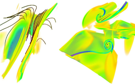
Figure 3: (Color online) Regions of strong current density, and magnetic field lines in their vicinity for run RND5 at $t=1.6$. The region at left has $450^{2}\times 250$ points, and that at right has $260\times 160\times 200$. The sheets are thin and elongated (up to 1/3 the size of the box); the magnetic field lines are parallel to the sheet and quasi-orthogonal to each other on each side of it, and they depart from the sheet transversally. Both folding (left) and rolling (right) occurs at this $R_{e}$. Vortex sheets (not shown) are co-located and parallel to the current sheets.

The structures that develop appear to be accumulations of current sheets (similarly for the vorticity, not shown), as was already found in PPS95 . Figure 3 shows a zoom on two such structures, with the magnetic field lines indicated as well. It appears clear from such figures that only one component of the magnetic field reverses sign in most of these configurations, reminiscent of magnetospheric observations. Both terms appearing in Eq. (3) for the dynamical evolution of $\omega^{\pm}$ are substantial and comparable in magnitude although they may be quite weak elsewhere in the flow. Kelvin-Helmoltz instabilities with rolling up of such sheets are also present in the flow but only at the highest Reynolds number (run RND5); at lower $R_{e}$ the sheets are thicker, the instability is too slow and only folding of such sheets occur. Magnetic field lines are parallel to the roll, in such a way that magnetic tension does not prevent the occurrence of the instability. Note that folding of magnetic structures has been advocated in the context of MHD at large magnetic Prandtl number cowley . Alfvenization of the flow ($\mathbf{v}=\pm\mathbf{b}$) is rather strong in the vicinity of the sheets, with $0.7\leq|{\tilde{\rho}}^{c}|\leq 1$, although globally the flow remains uncorrelated (${\tilde{\rho}}^{c}\sim 4\times 10^{-4}$); this local Alfvenization gives stability to such structures since the nonlinear terms are weakened, in much the same way vortex tubes in Navier-Stokes flows are long-lived because of (partial) Beltramization ($\mathbf{v}\sim\pm\mbox{\boldmath$\omega$}$). Moreover, within the sheet ${\tilde{\rho}}^{c}$ is positive, and it is negative outside, with a slight predominance of $\mathbf{b}$. All this indicates that a double velocity-magnetic field shear plays an important role in the development of small scales in MHD.

There is an elementary, analytically-soluble, one-dimensional model that illustrates sharply the role that velocity shear can play in enhancing current intensity, e.g. during early dynamo activity montgo . This consists of two semi-infinite slabs of rigid metal with equal conductivities, at rest against each other at the plane $y=0$, say. A uniform dc magnetic field ${\bf b}_{0}$ is perpendicular to the interface and penetrates both slabs. At time $t=0$, the slabs are impulsively forced to slide past each other in the $x$-direction with equal and opposite velocities (${\bf v}_{0}$, say). The developing (quasi-magnetostatic) field, which acquires an $x$-component, is a function of $y$ and $t$ only, and is governed by diffusion equations above and below the plane $y=0$. Matching tangential components of the electric field immediately above and below the interface reduces the pair to a soluble diffusion equation with a fixed $y$-derivative at $y=0$. The resulting magnetic field is expressible in terms of complementary error functions and grows without bound, as does the total Ohmic dissipation. The introduction of a time dependence in ${\bf v}_{0}$ may allow also for solutions in which the maximum of the current grows as a power law in time.

In conclusion, high resolution simulations of the early stages in the development of MHD turbulence allowed us to study the creation and evolution of small scale structures in three-dimensional flows. Roll up of current and vortex sheets, and a self-similar growth of current and vorticity maxima was found, features that to the best of our knowledge were not observed in previous simulations at smaller Reynolds numbers. Also, a convergence of the maximum dissipation rate to a value independent of $R_{e}$ was found. More analysis will be carried out to understand how structures are formed, the relevance of the development of alignment between the fields and the creation and role of local exact solutions to the MHD equations (such as Alfvén waves).

NSF grants CMG-0327888 and ATM-0327533 are acknowledged. Computer time provided by NCAR. Three-dimensional visualizations were done using VAPoR. vapor .

References

- (1) H. Politano, A. Pouquet, and V. Carbone, EuroPhys. Lett. 43, 516 (1988).
- (2) J. Greene, J. Geophys. Res. 93, 8583 (1988).
- (3) J. Beale, T. Kato, and A. Majda, Comm. Math. Phys. 94, 61 (1984).
- (4) R. Catflisch, I. Klapper, and G. Steele, Comm. Math. Phys. 184, 443 (1997).
- (5) H. Politano, A. Pouquet, and P.L. Sulem, Phys. Plasmas 2, 2931 (1995).
- (6) R. Kerr and A. Brandenburg, Phys. Rev. Lett. 83, 1155 (1999); see also arXiv:physics/0001016 (2000).
- (7) R. Grauer and C. Marliani, Phys. Rev. Lett. 84, 4850 (2000).
- (8) R. Kerr, Phys. Fluids A17, 075103 (2005).
- (9) N. Wild, W. Gekelman, and R. Stenzel, Phys. Rev. Lett., 46, 339 (1981); A.C. Ting, W.H. Matthaeus, and D. Montgomery, Phys. Fluids 29, 3261 (1983); Y. Ono, M. Yamada, T. Akao, T. Tajima and R. Matsumoto, Phys. Rev. Lett. 76, 3328 (1996); D. Knoll and J. Brackbill, Phys. Plasmas 9, 3775 (2002).
- (10) I. Syrovatskii, Sov. Phys. JETP 33, 933 (1971).
- (11) A. Pouquet, in European School in Astrophysics, C. Chiuderi and G. Einaudi Eds, Springer-Verlag, Lecture Notes in Physics 468, 163 (1996).
- (12) U. Frisch, A. Pouquet, P.L. Sulem, and M. Meneguzzi, J. Mécanique Théor. Appl., 2, 191 (1983).
- (13) I. Klapper, A. Rado and M. Tabor, Phys. Plasmas 3, 4281 (1996).
- (14) D. Biskamp and H. Welter, Phys. Fluids B1, 1964 (1989); H. Politano, A. Pouquet, and P.L. Sulem, Phys. Fluids B1, 2330 (1989).
- (15) Or their combinations in terms of the pseudo-energies of the Elsässer variables .
- (16) One may also monitor the temporal development of the symmetrized velocity and magnetic field gradient matrices, as well as that of the total enstrophy production kerrB1 .
- (17) S. Orszag, and C.-M. Tang, J. Fluid Mech. 90, 129 (1979).
- (18) J. Picone, and R. Dahlburg, Phys. Fluids B3, 29 (1991).
- (19) E. Priest and T. Forbes, “Magnetic reconnection: MHD Theory and Applications”, Cambridge U. Press (2000).
- (20) A. Alexakis, P.D. Mininni, and A. Pouquet, Phys. Rev. E 72, 046301; P.D. Mininni, A. Alexakis, and A. Pouquet, Phys. Rev. E 72, 046302.
- (21) V.I. Arnol’d, C. R. Acad. Sci. Paris 261, 17 (1965); D. Galloway and U. Frisch, Geophys. Astrophys. Fluid Dyn 36, 58 (1986).
- (22) A. Schekochihin et al., Astrophys. J. 576 806 (2002).
- (23) D.C. Montgomery, P.D. Mininni, and A. Pouquet, Bull. Am. Phys. Soc., Ser. II, 50(8), 177 (2005).
- (24) J. Clyne and M. Rast, in Visualization and data analysis 2005, R.F. Erbacher et al. (Eds.), SPIE, Bellingham, Wash. (2005), 284; http://www.vapor.ucar.edu.