Electrical control of the linear optical properties of particulate composite materials

Akhlesh Lakhtakia^a and Tom G. Mackay^b

^a CATMAS — Computational & Theoretical Materials Sciences Group
Department of Engineering Science & Mechanics
212 Earth & Engineering Sciences Building
Pennsylvania State University, University Park, PA 16802–6812, USA
email: akhlesh@psu.edu

^b School of Mathematics
James Clerk Maxwell Building
University of Edinburgh
Edinburgh EH9 3JZ, United Kingdom
email: T.Mackay@ed.ac.uk

Abstract

The Bruggeman formalism for the homogenization of particulate composite materials is used to predict the effective permittivity dyadic of a two–constituent composite material with one constituent having the ability to display the Pockels effect. Scenarios wherein the constituent particles are randomly oriented, oriented spheres, and oriented spheroids are numerically explored. Thereby, homogenized composite materials (HCMs) are envisaged whose constitutive parameters may be continuously varied through the application of a low–frequency (dc) electric field. The greatest degree of control over the HCM constitutive parameters is achievable when the constituents comprise oriented and highly aspherical particles and have high electro–optic coefficients.

Keywords: Bruggeman formalism, composite material, electro–optics, homogenization, particulate material, Pockels effect

1 Introduction

In 1806, after having ascended the skies in a balloon to collect samples of air at different heights and after having ascertained the proportions of different gases in each sample, Jean–Baptiste Biot and François Arago published the first known homogenization formula for the refractive index of a mixture of mutually inert gases as the weighted sum of their individual refractive indexes, the weights being in ratios of their volumetric proportions in the mixture (Biot & Arago 1806). The Arago–Biot mixture formula heralded the science and technology of particulate composite materials — particularly in optics, more generally in electromagnetics, and even more generally in many other branches of physics. An intensive literature has developed over the last two centuries in optics (Neelakanta 1995; Lakhtakia 1996), and recent forays into the realms of metamaterials and complex mediums (Grimmeiss et al. 2002; Weiglhofer & Lakhtakia 2003; Mackay 2005) have reaffirmed the continued attraction of both particulate composite materials and homogenization formalisms.

Post–fabrication dynamic control of the effective properties of a mixture of two constituent materials is a technologically important capability underlying the successful deployment of a host of smart materials and structures. Dynamic control can be achieved in many ways, particularly if controlability and sensing capablity are viewed as complementary attributes. One way is to infiltrate the composite material with another substance, possibly a fluid, to change, say, the effective optical response properties (Lakhtakia et al. 2001; Mönch et al. 2006). This can be adequate if rapidity of change is not a critical requirement. Another way is to tune the effective properties by the application of pressure (Finkelmann et al. 2001; Wang et al. 2003) or change of temperature (Schadt & Fünfschilling 1990). Faster ways of dynamic control could involve the use of electric fields if one constituent material is a liquid crystal (Yu et al. 2005) or magnetic fields if one constituent material is magnetic (Shafarman et al. 1986).

Our focus in this paper is the control of the effective permittivity tensor of a two–constituent composite material, wherein both constituent materials are classified as dielectric materials in the optical regime but one can display the Pockels effect (Boyd 1992). Both constituent materials can be distributed as ellipsoidal particles whose orientations can be either fixed or be completely random.

The plan of this paper is as follows: Section 2 contains a description of the particulate composite material of interest, as well as the key equations of the Bruggeman homogenization formalism (Bruggeman 1935; Weiglhofer et al. 1997) adopted to estimate the relative permittivity dyadic of the homogenized composite material (HCM). Section 3 presents a few numerical examples to show that the Pockels effect can be exploited to dynamically control the linear optical response properties of composite materials through a low–frequency electric field. Given the vast parameter space underlying the Pockels effect, we emphasize that the examples presented are merely illustrative. Some brief concluding remarks are provided in Section 4.

A note about notation: Vectors are in boldface, dyadics are double underlined. A Cartesian coordinate system with unit vectors ${\bf u}_{x,y,z}$ is adopted. The identity dyadic is written as $\underline{\underline{I}}$, and the null dyadic as $\underline{\underline{0}}$. An $\exp(-i\omega t)$ time–dependence is implicit with $i=\sqrt{-1}$, $\omega$ as angular frequency, and $t$ as time.

2 Theory

Let the two constituent materials of the particulate composite material be labeled $a$ and $b$. Their respective volumetric proportions are denoted by $f_{a}$ and $f_{b}=1-f_{a}$. They are distributed as ellipsoidal particles. The dyadic

$$\underline{\underline{U}}^{(a)}=\sum_{K=1}^{3}\,\alpha_{K}\,{\bf a}_{K}{\bf a}_{K}$$ (1)

describes the shape of particles made of material $a$, with $\alpha_{K}>0\,\forall K\in\left[1,3\right]$ and the three unit vectors ${\bf a}_{1,2,3}$ being mutually orthogonal. The shape dyadic

$$\underline{\underline{U}}^{(b)}=\sum_{K=1}^{3}\,\beta_{K}\,{\bf b}_{K}{\bf b}_{K}$$ (2)

similarly describes the shape of the particles made of material $b$. A low–frequency (or dc) electric field ${\bf E}^{dc}$ acts on the composite material, the prediction of whose effective permittivity dyadic in the optical regime is of interest.

Material $a$ does not display the Pockels effect and, for simplicity, we take it to be isotropic with relative permittivity scalar $\epsilon^{(a)}$ in the optical regime.

Material $b$ has more complicated dielectric properties as it displays the Pockels effect. Its linear electro–optic properties are expressed through the inverse of its relative permittivity dyadic in the optical regime, which is written as (Boyd 1992)

$$\left[\underline{\underline{\epsilon}}^{(b)}\right]^{-1} = \sum_{K=1}^{3}\left[\left(1/\epsilon_{K}^{(b)}+s_{j}\right)\,{\bf u}_{K}{\bf u}_{K}\right]$$ (3)

$$+ s_{4}\left({\bf u}_{2}{\bf u}_{3}+{\bf u}_{3}{\bf u}_{2}\right)+s_{5}\left({\bf u}_{1}{\bf u}_{3}+{\bf u}_{3}{\bf u}_{1}\right)+s_{6}\left({\bf u}_{1}{\bf u}_{2}+{\bf u}_{2}{\bf u}_{1}\right)\,,$$

where

$$s_{J}=\sum_{K=1}^{3}r_{JK}\,E_{K}^{dc}\,,\quad J\in\left[1,6\right]\,,$$ (4)

and the unit vectors

$$\left.\begin{array}[]{l}{\bf u}_{1}=-({\bf u}_{x}\cos\phi_{b}+{\bf u}_{y}\sin\phi_{b})\cos\theta_{b}+{\bf u}_{z}\sin\theta_{b}\\[5.0pt] {\bf u}_{2}={\bf u}_{x}\sin\phi_{b}-{\bf u}_{y}\cos\phi_{b}\\[5.0pt] {\bf u}_{3}=({\bf u}_{x}\cos\phi_{b}+{\bf u}_{y}\sin\phi_{b})\sin\theta_{b}+{\bf u}_{z}\cos\theta_{b}\end{array}\right\}\,,\quad\theta_{b}\in\left[0,\pi\right]\,,\quad\phi_{b}\in\left[0,2\pi\right]\,,$$ (5)

are relevant to the crystallographic structure of the material. In (3) and (4), $E_{K}^{dc}={\bf u}_{K}\mbox{ \tiny{${}^{\bullet}$} }{\bf E}^{dc}$, $K\in\left[1,3\right]$, are the Cartesian components of the dc electric field; $\epsilon_{1,2,3}^{(b)}$ are the principal relative permittivity scalars in the optical regime; and $r_{JK}$, $J\in\left[1,6\right]$ and $K\in\left[1,3\right]$, are the $18$ electro–optic coefficients in the traditional contracted or abbreviated notation for representing symmetric second–order tensors (Auld 1990). Correct to the first order in the components of the dc electric field, which is commonplace in electro–optics (Yariv & Yeh 2007), we get the linear approximation (Lakhtakia 2006a)

$$\underline{\underline{\epsilon}}^{(b)} \approx \sum_{K=1}^{3}\left[\epsilon_{K}^{(b)}\left(1-\epsilon_{K}^{(b)}s_{K}\right)\,{\bf u}_{K}{\bf u}_{K}\right]$$ (6)

$$- \epsilon_{2}^{(b)}\epsilon_{3}^{(b)}\,s_{4}\left({\bf u}_{2}{\bf u}_{3}+{\bf u}_{3}{\bf u}_{2}\right)-\epsilon_{1}^{(b)}\epsilon_{3}^{(b)}\,s_{5}\left({\bf u}_{1}{\bf u}_{3}+{\bf u}_{3}{\bf u}_{1}\right)-\epsilon_{1}^{(b)}\epsilon_{2}^{(b)}\,s_{6}\left({\bf u}_{1}{\bf u}_{2}+{\bf u}_{2}{\bf u}_{1}\right)$$

from (3), provided that

$$\left\{{\begin{subarray}{c}\max\\ K\in\left[1,3\right]\end{subarray}}\,\lvert\epsilon_{K}^{(b)}\rvert\right\}\,\,\left\{{\begin{subarray}{c}\max\\ J\in\left[1,6\right]\end{subarray}}\,\lvert s_{J}\rvert\right\}\ll 1\,.$$ (7)

This material can be isotropic, uniaxial, or biaxial, depending on the relative values of $\epsilon_{1}^{(b)}$, $\epsilon_{2}^{(b)}$, and $\epsilon_{3}^{(b)}$. Furthermore, this material may belong to one of 20 crystallographic classes of point group symmetry, in accordance with the relative values of the electro–optic coefficients.

Let the Bruggeman estimate of the relative permittivity dyadic of HCM be denoted by $\underline{\underline{\epsilon}}^{Br}$. If the particles of material $a$ are all identically oriented with respect to their crystallographic axes, and likewise the particles of material $b$, then $\underline{\underline{\epsilon}}^{Br}$ is determined by solving the following equation (Weiglhofer et al. 1997):

$$f_{a}\left(\epsilon^{(a)}\underline{\underline{I}}-\underline{\underline{\epsilon}}^{Br}\right)\mbox{ \tiny{${}^{\bullet}$} }\left[\underline{\underline{I}}+\underline{\underline{d}}^{(a)}\mbox{ \tiny{${}^{\bullet}$} }\left(\epsilon^{(a)}\underline{\underline{I}}-\underline{\underline{\epsilon}}^{Br}\right)\right]^{-1}$$

$$\qquad\quad+f_{b}\left(\underline{\underline{\epsilon}}^{(b)}-\underline{\underline{\epsilon}}^{Br}\right)\mbox{ \tiny{${}^{\bullet}$} }\left[\underline{\underline{I}}+\underline{\underline{d}}^{(b)}\mbox{ \tiny{${}^{\bullet}$} }\left(\underline{\underline{\epsilon}}^{(b)}-\underline{\underline{\epsilon}}^{Br}\right)\right]^{-1}=\underline{\underline{0}}\,.$$ (8)

In this equation, $\underline{\underline{d}}^{a}\equiv\underline{\underline{d}}(\underline{\underline{U}}^{(a)})$ and $\underline{\underline{d}}^{b}\equiv\underline{\underline{d}}(\underline{\underline{U}}^{(b)})$, where the dyadic function

$$\underline{\underline{d}}(\underline{\underline{U}})=\frac{1}{4\pi}\int_{\phi_{q}=0}^{2\pi}\int_{\theta_{q}=0}^{\pi}\sin\theta_{q}\,\frac{\underline{\underline{U}}^{-1}\mbox{ \tiny{${}^{\bullet}$} }{\bf q}{\bf q}\mbox{ \tiny{${}^{\bullet}$} }\underline{\underline{U}}^{-1}}{{\bf q}\mbox{ \tiny{${}^{\bullet}$} }\underline{\underline{U}}^{-1}\mbox{ \tiny{${}^{\bullet}$} }\underline{\underline{\epsilon}}^{Br}\mbox{ \tiny{${}^{\bullet}$} }\underline{\underline{U}}^{-1}\mbox{ \tiny{${}^{\bullet}$} }{\bf q}}\,d\theta_{q}\,d\phi_{q}\,$$ (9)

contains the unit vector

$${\bf q}={\bf u}_{z}\cos\theta_{q}+({\bf u}_{x}\cos\phi_{q}+{\bf u}_{y}\sin\phi_{q})\,\sin\theta_{q}\,.$$ (10)

The Bruggeman formalism is more complicated when the relative permittivity dyadics of the particles of material $b$ are randomly oriented. To begin with, let there be $P\geq 1$ distinct orientations. We represent the p^th orientation of the relative permittivity dyadic $\underline{\underline{\epsilon}}^{(b)}$ in terms of the set of Euler angles $\left\{\gamma_{n_{p}}\right\}_{n=1}^{3}$ as (Lakhtakia 1993)

$$\underline{\underline{\epsilon}}^{(b)}_{p}=\underline{\underline{R}}_{\,z}(\gamma_{3_{p}})\mbox{ \tiny{${}^{\bullet}$} }\underline{\underline{R}}_{\,y}(\gamma_{2_{p}})\mbox{ \tiny{${}^{\bullet}$} }\underline{\underline{R}}_{\,z}(\gamma_{1_{p}})\mbox{ \tiny{${}^{\bullet}$} }\underline{\underline{\epsilon}}^{(b)}\mbox{ \tiny{${}^{\bullet}$} }\underline{\underline{R}}_{\,z}^{-1}(\gamma_{1_{p}})\mbox{ \tiny{${}^{\bullet}$} }\underline{\underline{R}}_{\,y}^{-1}(\gamma_{2_{p}})\mbox{ \tiny{${}^{\bullet}$} }\underline{\underline{R}}_{\,z}^{-1}(\gamma_{3_{p}})\,,\qquad p=1,2,3,.....,P,$$ (11)

wherein the rotational dyadics

$$\left.\begin{array}[]{l}\underline{\underline{R}}_{\,y}(\gamma)=\left({\bf u}_{x}\,{\bf u}_{x}+{\bf u}_{z}\,{\bf u}_{z}\right)\cos\gamma+\left({\bf u}_{z}\,{\bf u}_{x}-{\bf u}_{x}\,{\bf u}_{z}\right)\sin\gamma+{\bf u}_{y}\,{\bf u}_{y}\vspace{2mm}\\ \underline{\underline{R}}_{\,z}(\gamma)=\left({\bf u}_{x}\,{\bf u}_{x}+{\bf u}_{y}\,{\bf u}_{y}\right)\cos\gamma+\left({\bf u}_{x}\,{\bf u}_{y}-{\bf u}_{y}\,{\bf u}_{x}\right)\sin\gamma+{\bf u}_{z}\,{\bf u}_{z}\end{array}\right\}.$$ (12)

Let us define

$$\underline{\underline{\Pi}}(\gamma_{1_{p}},\gamma_{2_{p}},\gamma_{3_{p}})=\left(\underline{\underline{\epsilon}}^{(b)}_{p}-\underline{\underline{\epsilon}}^{Br}\right)\mbox{ \tiny{${}^{\bullet}$} }\left[\underline{\underline{I}}+\underline{\underline{d}}^{(b)}\mbox{ \tiny{${}^{\bullet}$} }\left(\underline{\underline{\epsilon}}^{(b)}_{p}-\underline{\underline{\epsilon}}^{Br}\right)\right]^{-1}.$$ (13)

Then the Bruggeman equation may be expressed in the form

$$f_{a}\left(\epsilon^{(a)}\underline{\underline{I}}-\underline{\underline{\epsilon}}^{Br}\right)\mbox{ \tiny{${}^{\bullet}$} }\left[\underline{\underline{I}}+\underline{\underline{d}}^{(a)}\mbox{ \tiny{${}^{\bullet}$} }\left(\epsilon^{(a)}\underline{\underline{I}}-\underline{\underline{\epsilon}}^{Br}\right)\right]^{-1}+f_{b}\frac{1}{P}\,\sum_{p=1}^{P}\,\underline{\underline{\Pi}}(\gamma_{1_{p}},\gamma_{2_{p}},\gamma_{3_{p}})=\underline{\underline{0}}\,,$$ (14)

if all $P$ orientations are equiprobable. In the limit $P\rightarrow\infty$, equation (14) becomes

$$f_{a}\left(\epsilon^{(a)}\underline{\underline{I}}-\underline{\underline{\epsilon}}^{Br}\right)\mbox{ \tiny{${}^{\bullet}$} }\left[\underline{\underline{I}}+\underline{\underline{d}}^{(a)}\mbox{ \tiny{${}^{\bullet}$} }\left(\epsilon^{(a)}\underline{\underline{I}}-\underline{\underline{\epsilon}}^{Br}\right)\right]^{-1}$$

$$\qquad\quad+\frac{f_{b}}{8\pi^{2}}\int^{2\pi}_{\gamma_{3}=0}\int^{\pi}_{\gamma_{2}=0}\int^{2\pi}_{\gamma_{3}=0}\,\underline{\underline{\Pi}}(\gamma_{1},\gamma_{2},\gamma_{3})\,\sin\gamma_{2}\;d\gamma_{1}\,d\gamma_{2}\,d\gamma_{3}=\underline{\underline{0}}\,.$$ (15)

Even more complicated orientational averages — e.g., of particulate shapes and geometric orientation of particles, in addition to crystallographic orientation — can be similarly handled.

The HCM relative permittivity $\underline{\underline{\epsilon}}^{Br}$ can be extracted from equation (8) and equation (15) iteratively using standard techniques, and a Jacobi iteration technique is recommended (Michel 2000).

3 Numerical results and discussion

A vast parameter space is covered by the homogenization formalism described in the previous section. The parameters include: the volumetric proportions and the shape dyadics of materials $a$ and $b$; the relative permittivity scalar $\epsilon^{(a)}$; the three relative permittivity scalars $\epsilon_{K}^{(b)}$ and the upto 18 distinct electro–optic coefficients $r_{JK}$ of material $b$; the angles $\theta_{b}$ and $\phi_{b}$ that describe the crystallographic orientation of material $b$ with respect to the laboratory coordinate system; and the magnitude and direction of ${\bf E}^{dc}$. To provide illustrative results here, we set $\epsilon^{(a)}=1$. All calculations were made for two choices of material $b$ (Cook 1996):

• zinc telluride, which belongs to the cubic ${\bar{4}}3m$ crystallographic class: $\epsilon_{1}^{(b)}=\epsilon_{2}^{(b)}=\epsilon_{3}^{(b)}=8.94$, $r_{41}=r_{52}=r_{63}=4.04\times 10^{-12}$ m V^-1, and all other $r_{JK}\equiv 0$; and

• potassium niobate, which belongs to the orthorhombic $mm2$ crystallographic class: $\epsilon_{1}^{(b)}=4.72$, $\epsilon_{2}^{(b)}=5.20$, $\epsilon_{3}^{(b)}=5.43$, $r_{13}=34\times 10^{-12}$ m V^-1, $r_{23}=6\times 10^{-12}$ m V^-1, $r_{33}=63.4\times 10^{-12}$ m V^-1, $r_{42}=450\times 10^{-12}$ m V^-1, $r_{51}=120\times 10^{-12}$ m V^-1, and all other $r_{JK}\equiv 0$.

Given the huge parameter space still left, we chose to fix $f_{b}=0.5$, the Bruggeman formalism then being maximally distinguished from other homogenization formalisms such as the Maxwell Garnett (Weiglhofer et al. 1997) and the Bragg–Pippard formalisms (Bragg & Pippard 1953; Sherwin & Lakhtakia 2002). Finally, we chose particles of material $a$ and $b$ to be spherical (i.e., $\underline{\underline{U}}^{(a)}=\underline{\underline{U}}^{(b)}=\underline{\underline{I}}$) in Sections 3.1 and 3.2, and spheroidal in Section 3.3.

Two different scenarios based on the orientation of material $b$ were investigated. The scenario wherein the material $b$ particles are randomly oriented with respect to their crystallographic axes was considered in the study presented in Section 3.1. Particles of material $b$ were taken to have the same orientation with respect to their crystallographic axes in the studies presented in Sections 3.2 and 3.3.

For all scenarios, the estimated permittivity dyadic of the HCM may be compactly represented as

$$\underline{\underline{\epsilon}}^{Br}=\alpha^{Br}\,\underline{\underline{I}}+\beta^{Br}\,({\bf u}_{M}{\bf u}_{N}+{\bf u}_{N}{\bf u}_{M}),$$ (16)

wherein the unit vectors ${\bf u}_{M}$ and ${\bf u}_{N}$ are aligned with the optic ray axes of the HCM (Chen 1983; Weiglhofer & Lakhtakia 1999; Mackay & Weiglhofer 2001). For the real–symmetric relative permittivity dyadic $\underline{\underline{\epsilon}}^{Br}$, with three distinct (and orthonormalised) eigenvectors ${\bf e}_{1,2,3}$ and corresponding eigenvalues $\epsilon_{1,2,3}^{Br}$, the scalars $\alpha^{Br}$ and $\beta^{Br}$ are given by

$$\left.\begin{array}[]{l}\alpha^{Br}=\epsilon_{2}^{Br}\\[5.0pt] \beta^{Br}=\displaystyle{\frac{\epsilon_{3}^{Br}-\epsilon_{1}^{Br}}{2}}\end{array}\right\},$$ (17)

whereas the unit vectors ${\bf u}_{M,N}$ may be stated as

$$\left.\begin{array}[]{l}{\bf u}_{M}=\displaystyle{\left(\frac{\epsilon_{2}^{Br}-\epsilon_{1}^{Br}}{\epsilon_{3}^{Br}-\epsilon_{1}^{Br}}\right)^{1/2}{\bf e}_{1}+\left(\frac{\epsilon_{3}^{Br}-\epsilon_{2}^{Br}}{\epsilon_{3}^{Br}-\epsilon_{1}^{Br}}\right)^{1/2}{\bf e}_{3}\vspace{2mm}}\\ {\bf u}_{N}=\displaystyle{-\left(\frac{\epsilon_{2}^{Br}-\epsilon_{1}^{Br}}{\epsilon_{3}^{Br}-\epsilon_{1}^{Br}}\right)^{1/2}{\bf e}_{1}+\left(\frac{\epsilon_{3}^{Br}-\epsilon_{2}^{Br}}{\epsilon_{3}^{Br}-\epsilon_{1}^{Br}}\right)^{1/2}{\bf e}_{3}}\end{array}\right\},$$ (18)

for $\epsilon_{1}^{Br}<\epsilon_{2}^{Br}<\epsilon_{3}^{Br}$.

In accordance with mineralogical literature (Klein & Hurlbut 1985), we define the linear birefringence

$$\delta_{n}=\left(\epsilon_{3}^{Br}\right)^{1/2}-\left(\epsilon_{1}^{Br}\right)^{1/2}\,,$$ (19)

the degree of biaxiality

$$\delta_{bi}=\left(\epsilon_{3}^{Br}\right)^{1/2}+\left(\epsilon_{1}^{Br}\right)^{1/2}-2\left(\epsilon_{2}^{Br}\right)^{1/2}\,,$$ (20)

and the angles

$$\left.\begin{array}[]{l}\delta=\displaystyle{\cos^{-1}\left[\left(\frac{\epsilon_{3}^{Br}-\epsilon_{2}^{Br}}{\epsilon_{3}^{Br}-\epsilon_{1}^{Br}}\right)^{1/2}\right]\vspace{2mm}}\\ \theta_{M}=\cos^{-1}{\bf u}_{M}\mbox{ \tiny{${}^{\bullet}$} }{\bf u}_{z}\vspace{2mm}\\ \theta_{N}=\cos^{-1}{\bf u}_{N}\mbox{ \tiny{${}^{\bullet}$} }{\bf u}_{z}\end{array}\right\}.$$ (21)

The linear birefringence $\delta_{n}$ is the difference between the largest and the smallest refractive indexes of the HCM; the degree of biaxiality $\delta_{bi}$ can be either positive or negative, depending on the numerical value of $\left(\epsilon_{2}^{Br}\right)^{1/2}$ with respect to the mean of $\left(\epsilon_{1}^{Br}\right)^{1/2}$ and $\left(\epsilon_{3}^{Br}\right)^{1/2}$; $2\delta$ is the angle between the two optic ray axes; and $\theta_{M,N}$ are the angles between the optic ray axes and the Cartesian $z$ axis. Thus, $\underline{\underline{\epsilon}}^{Br}$ can be specified by six real–valued parameters: $\epsilon^{Br}_{2}$, $\delta_{n}$, $\delta_{bi}$, $\delta$, and $\theta_{M,N}$, in a physically illuminating way.

3.1 Randomly oriented spherical electro–optic particles

We begin by considering the scenario wherein the particles of material $b$ are randomly oriented with respect to their crystallographic axes, and the particles of both materials are spherical. Accordingly, the HCM is an isotropic dielectric medium, characterized by the relative permittivity dyadic $\underline{\underline{\epsilon}}^{Br}=\epsilon^{Br}\underline{\underline{I}}$.

The Bruggeman estimate $\epsilon^{Br}$, as extracted from equation (15), is plotted in Figure 1 against $E^{dc}_{3}$, with $E^{dc}_{1,2}=0$. Material $b$ is zinc telluride for the upper graph and potassium niobate for the lower in this figure. The range for the magnitude of ${\bf E}^{dc}$ in Figure 1 — and for all subsequent figures — was chosen in order to comply with (7). In the case where material $b$ is zinc telluride, $\epsilon^{Br}$ varies only slightly as $E^{dc}_{3}$ changes, and $\epsilon^{Br}$ is insensitive to the sign of $\epsilon^{Br}$. A greater degree of sensitivity to $E^{dc}_{3}$ is observed for the HCM which arises when material $b$ is potassium niobate; in this case the HCM’s relative permittivity is also sensitive to the sign of $E^{dc}_{3}$, thereby underscoring the significance of crystallographic class of the electro–optic constituent material even when averaging over crystallographic orientation is physically valid.

3.2 Identically oriented spherical electro–optic particles

The scenario wherein all particles of material $b$ are taken to be identically oriented, with particles of both constituent materials being spherical, is now considered. Let us begin with the case where material $b$ is zinc telluride. This is an isotropic material when ${\bf E}^{dc}={\bf 0}$, but the anisotropy underlying the Pockels effect becomes evident on the application of the low–frequency electric field (Lakhtakia 2006b).

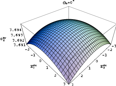
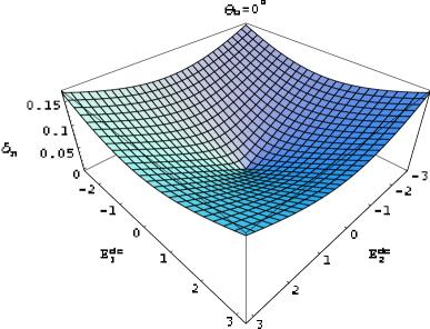
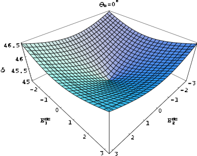
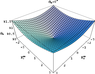
Figure 2: The HCM parameters $\epsilon^{Br}_{2}$, $\delta_{n}$, $\delta_{bi}$, $\delta$ (in degree) and $\theta_{M,N}$ (in degree) plotted against $E^{dc}_{1,2}$ (in V m^-1 $\times 10^{9}$). The crystallographic orientation angles of material $b$ are $\theta_{b}=\phi_{b}=0$; and $E^{dc}_{3}=0$. Material $b$ is zinc telluride, and the particles of both constituent materials are spherical.

The HCM parameters, as extracted from equation (8), are plotted in Figure 2 as functions of $E^{dc}_{1,2}$ with $E^{dc}_{3}=0$. The crystallographic orientation angles $\theta_{b}=\phi_{b}=0$. As expected, in this figure $\delta_{n}=\delta_{bi}=0$ (i.e., the HCM is isotropic) when $E^{dc}_{1}=E^{dc}_{2}=0$. The HCM constitutive parameters $\epsilon^{Br}_{2}$, $\delta_{n}$, $\delta_{bi}$, $\delta$, and $\theta_{M,N}$ are all insensitive to the signs of $E^{dc}_{1}$ and $E^{dc}_{2}$. The HCM is negatively biaxial in general (because $\delta_{bi}<0$), although the biaxiality is small. The linear birefringence is not sensitive to the signs of $E_{1,2}^{dc}$; it increases considerably as $|{\bf E}^{dc}|$ is increased, as a glance at data on minerals readily confirms (Griblle & Hall 1992). The two optic ray axes remain almost mutually orthogonal, as indicated by $\delta\approx 45^{\circ}$, as $|E_{1,2}^{dc}|$ are changed.

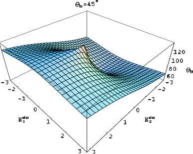
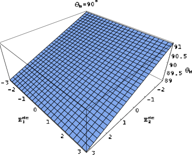
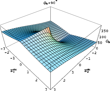
Figure 3: The optic ray axis angles $\theta_{M,N}$ (in degree) of the HCM plotted against $E^{dc}_{1,2}$ (in V m^-1 $\times 10^{9}$). The constitutive parameters of material $b$ are same as in Figure 2 except that $\theta_{b}\in\left\{45^{\circ},90^{\circ}\right\}$. (The corresponding plots of $\epsilon^{Br}_{2}$, $\delta_{n}$, $\delta_{bi}$, and $\delta$ are not noticeably different to those presented in Figure 2.)

The influence of the orientation angle $\theta_{b}$ for zinc telluride is explored in Figure 3. Here, the optic ray axis angles $\theta_{M,N}$ are plotted as functions of $E^{dc}_{1,2}$ with $E^{dc}_{3}=0$, for $\theta_{b}\in\left\{45^{\circ},90^{\circ}\right\}$ with $\phi_{b}=0$. The orientations of both optic ray axes continuously vary with increasing $E^{dc}_{1,2}$ in a manner which continuously varies as $\theta_{b}$ increases. The polar angle of the optic ray axis aligned with ${\bf u}_{M}$, namely $\theta_{M}$, is slightly sensitive to $E^{dc}_{2}$ but insensitive to $E^{dc}_{1}$. In contrast, $\theta_{N}$ is acutely sensitive to both $E^{dc}_{1}$ and $E^{dc}_{2}$. Furthermore, $\theta_{N}$ is sensitive to the sign of $E^{dc}_{2}$ but not the sign of $E^{dc}_{1}$. The HCM parameters $\epsilon^{Br}_{2}$, $\delta_{n}$, $\delta_{bi}$, $\delta$ — which are not presented in Figure 3 — are insensitive to increasing $\theta_{b}$; the plots for these quantities are not noticeably different from the corresponding plots presented in Figure 2.

Let us turn now to the case where material $b$ is potassium niobate. This material is anisotropic (orthorhombic and negatively biaxial) even when the Pockels effect is not invoked, and it has much higher electro–optic coefficients than zinc telluride — hence, it can be expected to lead a different palette of HCM properties.

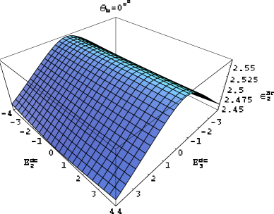
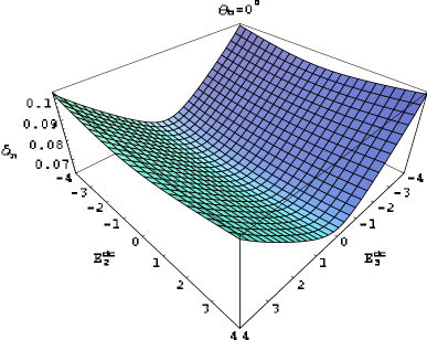
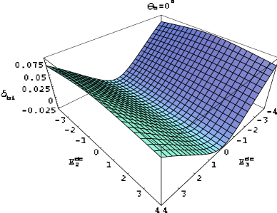
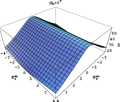
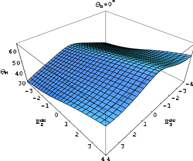
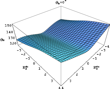
Figure 4: The HCM parameters $\epsilon^{Br}_{2}$, $\delta_{n}$, $\delta_{bi}$, $\delta$ (in degree) and $\theta_{M,N}$ (in degree) plotted against $E^{dc}_{2,3}$ (in V m^-1 $\times 10^{7}$). The crystallographic orientation angles of material $b$ are $\theta_{b}=\phi_{b}=0$; and $E^{dc}_{1}=0$. Material $b$ is potassium niobate, and the particles of both constituent materials are spherical.

The HCM parameters are plotted in Figure 4 as functions of $E^{dc}_{2,3}$ with $E^{dc}_{1}=0$. As in Figure 2, the crystallographic orientation angles of material $b$ are taken as $\theta_{b}=\phi_{b}=0$. Whereas the parameters $\epsilon^{Br}_{2}$, $\delta_{n}$, $\delta_{bi}$, and $\delta$ are not particularly sensitive to $E^{dc}_{2}$, they do vary significantly as $E^{dc}_{3}$ varies. Most notably, the HCM can be made either negatively biaxial ($\delta_{bi}<0$) or positively biaxial ($\delta_{bi}>0$). The two optic axes of the HCM need not be mutually orthogonal, with the included angle $2\delta$ between them as low as $40^{\circ}$. The polar angles $\theta_{M,N}$ are sensitive to both $E^{dc}_{2}$ and $E^{dc}_{3}$. We note that the sign of $E^{dc}_{3}$ does not influence any of the HCM parameters, but the sign of $E^{dc}_{2}$ does influence the polar angles $\theta_{M,N}$.

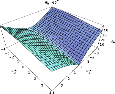
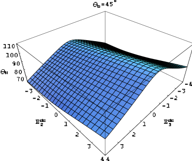
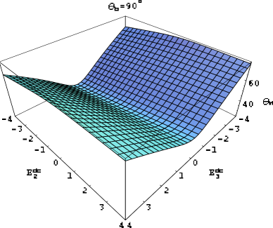
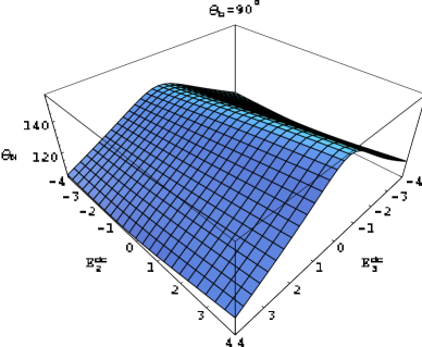
Figure 5: The optic ray axis angles $\theta_{M,N}$ (in degree) plotted against $E^{dc}_{2,3}$ (in V m^-1 $\times 10^{7}$). The constitutive parameters of material $b$ are same as in Figure 4 except that $\theta_{b}\in\left\{45^{\circ},90^{\circ}\right\}$. (The corresponding plots of $\epsilon^{Br}_{2}$, $\delta_{n}$, $\delta_{bi}$, and $\delta$ are not noticeably different to those presented in Figure 4.)

The influence of the orientation angle $\theta_{b}$ is explored in Figure 5. The constitutive parameters of material $b$ are the same as in Figure 4 but with $\theta_{b}\in\left\{45^{\circ},90^{\circ}\right\}$. As is the case in Figure 3, the graphs in Figure 5 show that the dependencies of the polar angles $\theta_{M,N}$ upon the components of ${\bf E}^{dc}$ are acutely sensitive to $\theta_{b}$. The HCM parameters $\epsilon^{Br}_{2}$, $\delta_{n}$, $\delta_{bi}$, and $\delta$ — which are not presented in Figure 5 — are insensitive to increasing $\theta_{b}$; the plots for these quantities are not noticeably different to the corresponding plots presented in Figure 4.

A comparison of Figures 2 and 3 with Figures 4 and 5 shows that the application of ${\bf E}^{dc}$ is more effective when material $b$ is potassium niobate rather than zinc telluride. A dc electric field that is two orders smaller in magnitude is required for changing the HCM properties with potassium niobate than with zinc telluride, and this observation is reaffirmed by comparing the upper and lower graphs in Figure 1. To a great extent, this is due to the larger electro–optic coefficients of potassium niobate; however, we cannot rule out some effect of the crystallographic structure of material $b$, which we plan to explore in the near future.

Electrical control appears to require dc electric fields of high magnitude. However, the needed dc voltages can be comparable with the half–wave voltages of electro–optic materials (Yariv & Yeh 2007). We must also note that the required magnitudes of ${\bf E}^{dc}$ are much smaller than the characteristic atomic electric field strength (Boyd 1992). The possibility of electric breakdown exists, but it would significantly depend on the time that the dc voltage would be switched on for. Finally, the non–electro–optic constituent material may have to be a polymer that can withstand high dc electric fields.

3.3 Identically oriented spheroidal electro–optic particles

We close by considering the scenario wherein the effect of the Pockels effect is going to be highly noticeable in the HCM — that is, when the particles of material $b$ are highly aspherical and the crystallographic orientation as well as the geometric orientation of these particles are aligned with ${\bf E}^{dc}$. We chose potassium niobate — which is more sensitive to the application of ${\bf E}^{dc}$ than zinc telluride — for our illustrative results.

In Figure 6, the HCM parameters $\epsilon^{Br}_{2}$, $\delta_{n}$, $\delta_{bi}$, $\delta$, and $\theta_{M}$ are plotted against $E^{dc}_{3}$, with $E^{dc}_{1,2}=0$. Both constituent materials are distributed as identical spheroids with shape parameters $\alpha_{1,2}=\beta_{1,2}=1$ and $\alpha_{3}=\beta_{3}\in\left\{3,6,9\right\}$; furthermore, $\theta_{b}=\phi_{b}=0$. As $\theta_{N}=180^{\circ}-\theta_{M}$ for this scenario, $\theta_{N}$ is not plotted. All the presented HCM parameters vary considerably as $E^{dc}_{3}$ increases; furthermore, all are sensitive to the sign of $E^{dc}_{3}$.

We note that the degree of biaxiality and the linear birefringence increase as $\alpha_{3}=\beta_{3}$ increases. This is a significant conclusion because perovskites (such as potassium niobate) are nowadays being deposited as oriented nanopillars (Gruverman & Kholkin 2006).

4 Concluding remarks

The homogenization of particulate composite materials with constituent materials that can exhibit the Pockels effect gives rise to HCMs whose effective constitutive parameters may be continuously varied through the application of a low–frequency (dc) electric field. Observable effects can be achieved even when the constituent particles are randomly oriented. Greater control over the HCM constitutive parameters may be achieved by orienting the constituent particles. By homogenizing constituent materials which comprise oriented elongated particles rather than oriented spherical particles, the degree of electrical control over the HCM constitutive parameters is further increased. The vast panoply of complex materials currently being investigated (Grimmeiss et al. 2002; Weiglhofer & Lakhtakia 2003; Mackay 2005; Mackay & Lakhtakia 2006) underscores the importance of electrically controlled composite materials for a host of applications for telecommunications, sensing, and actuation.

References

1. Auld, B.A. 1990 Acoustic fields and waves in solids. Malabar, FL, USA: Krieger.

2. Biot, J.–B. & Arago, F. 1806 Mémoire sur les affinités des corps pour la lumière et particulièrement sur les forces réfringentes des différents gaz. Mém. Inst. Fr. 7, 301–385.

3. Bruggeman, D.A.G. 1935 Berechnung verschiedener physikalischer Konstanten von Substanzen. I. Dielektrizitätskonstanten und Leitfähgkeiten der Mischkörper aus isotropen Substanzen. Ann. Phys. Lpz. 24, 636–679. [Facsimile reproduced in Lakhtakia (1996).]

4. Boyd, R.W. 1992 Nonlinear optics. San Diego, CA, USA: Academic Press.

5. Bragg, W.L. & Pippard, A.B. 1953 The form birefringence of macromolecules. Acta Crystallogr. 6, 865–867.

6. Chen, H.C. 1983 Theory of electromagnetic waves: A coordinate–free approach. New York, NY, USA: McGraw–Hill.

7. Cook Jr., W.R. 1996 Electrooptic coefficients, in: Nelson, D.F. (ed.), Landolt–Bornstein Volume III/30A. Berlin, Germany: Springer.

8. Finkelmann, H., Kim, S. T., Muñoz, A., Palffy–Muhoray, P. & Taheri, B. 2001 Tunable mirrorless lasing in cholesteric liquid crystalline elastomers. Adv. Mater. 13, 1069–1072.

9. Gribble, C.D. & Hall, A.J. 1992 Optical mineralogy: Principles & practice. London, United Kingdom: UCL Press.

10. Grimmeiss, H.G., Marletta, G., Fuchs, H. & Taga, Y. (eds.) 2002 Current trends in nanotechnologies: From materials to systems. Amsterdam, The Netherlands: Elsevier.

11. Gruverman, A. & Kholkin, A. 2006 Nanoscale ferroelectrics: processing, characterization, and future trends. Rep. Prog. Phys. 69, 2443–2474.

12. Klein, C. & Hurlbut, Jr., C.S. 1985 Manual of mineralogy. New York, NY, USA: Wiley. (pp. 247 et seq.)

13. Lakhtakia, A. 1993 Frequency–dependent continuum properties of a gas of scattering centers. Adv. Chem. Phys. 85(2), 311–359.

14. Lakhtakia, A. (ed.) 1996 Selected papers on linear optical composite materials. Bellingham, WA, USA: SPIE Optical Engineering Press.

15. Lakhtakia, A. 2006a Electrically tunable, ultranarrowband, circular–polarization rejection filters with electro–optic structurally chiral materials. J. Eur. Opt. Soc. – Rapid Pubs. 1, 06006.

16. Lakhtakia, A. 2006b Electrically switchable exhibition of circular Bragg phenomenon by an isotropic slab. Microw. Opt. Technol. Lett. 48, at press.

17. Lakhtakia, A., McCall, M.W., Sherwin, J.A., Wu, Q.H. & Hodgkinson, I.J. 2001 Sculptured–thin–film spectral holes for optical sensing of fluids. Opt. Commun. 194, 33–46.

18. Mackay, T.G. 2005 Linear and nonlinear homogenized composite mediums as metamaterials. Electromagnetics 25, 461–481.

19. Mackay, T.G. & Weiglhofer, W.S. 2001 Homogenization of biaxial composite materials: nondissipative dielectric properties. Electromagnetics 21, 15–26.

20. Mackay, T.G. & Lakhtakia, A. 2006 Electromagnetic fields in linear bianisotropic mediums. Prog. Opt. (at press).

21. Michel, B. 2000, Recent developments in the homogenization of linear bianisotropic composite materials. In: Singh, O.N. & Lakhtakia, A. 2000 Electromagnetic fields in unconventional materials and structures. New York, NY, USA: Wiley.

22. Mönch, W., Dehnert, J., Prucker, O., Rühe, J. & Zappe, H. 2006 Tunable Bragg filters based on polymer swelling. Appl. Opt. 45, 4284–4290.

23. Neelakanta, P.S. 1995 Handbook of electromagnetic materials — Monolithic and composite versions and their applications. Boca Raton, FL, USA: CRC Press.

24. Schadt, M. & Fünfschilling, J. 1990 New liquid crystal polarized color projection principle. Jap. J. Appl. Phys. 29, 1974–1984.

25. Shafarman, W.N., Castner, T.G., Brooks, J.S., Martin, K.P. & Naughton, M.J. 1986 Magnetic tuning of the metal–insulator transition for uncompensated arsenic–doped silicon. Phys. Rev. Lett. 56, 980–983.

26. Sherwin, J.A. & Lakhtakia, A. 2002 Bragg–Pippard formalism for bianisotropic particulate composites. Microw. Opt. Technol. Lett. 33, 40–44.

27. Yariv, A. & Yeh, P. 2007 Photonics: Optical electronics in modern communications, 6th ed. New York, NY, USA: Oxford University Press.

28. Yu, H., Tang, B.Y., Li, J. & Li, L. 2005 Electrically tunable lasers made from electro–optically active photonics band gap materials. Opt. Express 13, 7243–7249.

29. Wang, F., Lakhtakia, A. & Messier, R. 2003 On piezoelectric control of the optical response of sculptured thin films. J. Modern Opt. 50, 239–249.

30. Weiglhofer, W.S. & Lakhtakia, A. 1999 On electromagnetic waves in biaxial bianisotropic media. Electromagnetics 19, 351–362.

31. Weiglhofer, W.S. & Lakhtakia, A. (ed.) 2003 Introduction to complex mediums for optics and electromagnetics. Bellingham, WA, USA: SPIE Press.

32. Weiglhofer, W.S., Lakhtakia, A. & Michel, B. 1997 Maxwell Garnett and Bruggeman formalisms for a particulate composite with bianisotropic host medium. Microw. Opt. Technol. Lett. 15, 263–266; correction: 1999 22, 221.

Figure 1: The estimated relative permittivity scalar $\epsilon^{Br}$ of the HCM plotted against $E^{dc}_{3}$ (in V m^-1 $\times 10^{8}$) for $E^{dc}_{1,2}=0$ and $f_{a}=0.5$. Material $b$ is zinc telluride for the upper graph and potassium niobate for the lower graph. The particles of material $b$ are randomly oriented with respect to their crystallographic axes, and both types of particles are spherical.

Figure 6: The HCM scalar parameters $\epsilon^{Br}_{2}$, $\delta_{n}$, and $\delta_{bi}$, $\delta$ (in degree), and $\theta_{M}$ (in degree) plotted against $E^{dc}_{3}$ (in V m^-1 $\times 10^{8}$). The crystallographic orientation angles $\theta_{b}=\phi_{b}=0$, and $E^{dc}_{1,2}=0$. Material $b$ is potassium niobate. The constituent materials are distributed as spheroids with shape parameters: $\alpha_{1}=\alpha_{2}=\beta_{1}=\beta_{2}=1$; and $\alpha_{3}=\beta_{3}=3$ (solid curves), $\alpha_{3}=\beta_{3}=6$ (dashed curves), and $\alpha_{3}=\beta_{3}=9$ (broken dashed curves). The optic ray angle $\theta_{N}=180^{\circ}-\theta_{M}$.