Detrended fluctuation analysis for fractals and multifractals in higher dimensions

Abstract

One-dimensional detrended fluctuation analysis (1D DFA) and multifractal detrended fluctuation analysis (1D MF-DFA) are widely used in the scaling analysis of fractal and multifractal time series because of being accurate and easy to implement. In this paper we generalize the one-dimensional DFA and MF-DFA to higher-dimensional versions. The generalization works well when tested with synthetic surfaces including fractional Brownian surfaces and multifractal surfaces. The two-dimensional MF-DFA is also adopted to analyze two images from nature and experiment and nice scaling laws are unraveled.

I Introduction

Fractals and multifractals are ubiquitous in natural and social sciences Mandelbrot (1983). The most usual records of observable quantities are in the form of time series and their fractal and multifractal properties have been extensively investigated. There are many methods proposed for this purpose Taqqu et al. (1995); Montanari et al. (1999), such as spectral analysis, rescaled range analysis Hurst (1951); Mandelbrot and Van Ness (1968); Mandelbrot and Wallis (1969a, b, c, d), fluctuation analysis Peng et al. (1992), detrended fluctuation analysis Peng et al. (1994); Hu et al. (2001); Kantelhardt et al. (2002), wavelet transform module maxima (WTMM) Holschneider (1988); Muzy et al. (1991, 1993a, 1993b, 1994), detrended moving average Alessio et al. (2002); Carbone et al. (2004a, b); Alvarez-Ramirez et al. (2005); Xu et al. (2005), to list a few. It is now the common consensus that DFA and WTMM have the highest precision in the scaling analysis Taqqu et al. (1995); Montanari et al. (1999); Audit et al. (2002).

The idea of DFA was invented originally to investigate the long-range dependence in coding and noncoding DNA nucleotides sequence Peng et al. (1994). Then it was generalized to study the multifractal nature hidden in time series, termed as multifractal DFA (MF-DFA) Kantelhardt et al. (2002). Due to the simplicity in implementation, the DFA is now becoming the most important method in the field.

Although the WTMM method seems a little bit complicated, it is no doubt a very powerful method, especially for high-dimensional objects, such as images, scalar and vector fields of three-dimensional turbulence Arnéodo et al. (2000); Decoster et al. (2000); Roux et al. (2000); Kestener and Arneodo (2003, 2004). In contrast, the original DFA method is not designed for such purpose. In a recent paper, a first effort is taken to apply DFA to study the roughness features of texture images Alvarez-Ramirez et al. (2006). Specifically, the DFA is applied to extract Hurst indices of the one-dimensional sequences at different image orientations and their average scaling exponent is estimated. Unfortunately, this is nevertheless a one-dimensional DFA method.

In this work, we generalize the DFA (and MF-DFA as well) method from one-dimensional to high-dimensional. The generalized methods are tested by synthetic surfaces (fractional Brownian surfaces and multifractal surfaces) with known fractal and multifractal properties. The numerical results are in excellent agreement with the theoretical properties. We then apply these methods to practical examples. We argue that there are tremendous potential applications of the generalized DFA to many objects, such as the roughness of fracture surfaces, landscapes, clouds, three-dimensional temperature fields and concentration fields, turbulence velocity fields.

The paper is organized as follows. In Sec. II, we represent the algorithm of the two-dimensional detrended fluctuation analysis and the two-dimensional multifractal detrended fluctuation analysis. Section III shows the results of the numerical simulations, which are compared with theoretical properties. Applications to practical examples are illustrated in Sec. IV. We discuss and conclude in Sec. V.

II Method

II.1 Two-dimensional DFA

Being a direct generalization, the higher-dimensional DFA and MF-DFA have quite similar procedures as the one-dimensional DFA. We shall focus on two-dimensional space and the generalization to higher-dimensional is straightforward. The two-dimensional DFA consists of the following steps.

Step 1: Consider a self-similar (or self-affine) surface, which is denoted by a two-dimensional array $X(i,j)$, where $i=1,2,\cdots,M$, and $j=1,2,\cdots,N$. The surface is partitioned into $M_{s}\times N_{s}$ disjoint square segments of the same size $s\times s$, where $M_{s}=[M/s]$ and $N_{s}=[N/s]$. Each segment can be denoted by $X_{v,w}$ such that $X_{v,w}(i,j)=X(l_{1}+i,l_{2}+j)$ for $1\leqslant{i,j}\leqslant{s}$, where $l_{1}=(v-1)s$ and $l_{2}=(w-1)s$.

Step 2: For each segment $X_{v,w}$ identified by $v$ and $w$, the cumulative sum $u_{v,w}(i,j)$ is calculated as follows:

$$u_{v,w}(i,j)=\sum_{k_{1}=1}^{i}\sum_{k_{2}=1}^{j}{X_{v,w}(k_{1},k_{2})}~{},$$ (1)

where $1\leqslant{i,j}\leqslant{s}$. Note that $u_{v,w}$ itself is a surface.

Step 3: The trend of the constructed surface $u_{v,w}$ can be determined by fitting it with a prechosen bivariate polynomial function $\widetilde{u}$. The simplest function could be a plane. In this work, we shall adopt the following five detrending functions to test the validation of the methods:

$$\widetilde{u}_{v,w}(i,j) = ai+bj+c~{},$$ (2)

$$\widetilde{u}_{v,w}(i,j) = ai^{2}+bj^{2}+c~{},$$ (3)

$$\widetilde{u}_{v,w}(i,j) = aij+bi+cj+d~{},$$ (4)

$$\widetilde{u}_{v,w}(i,j) = ai^{2}+bj^{2}+ci+dj+e~{},$$ (5)

$$\widetilde{u}_{v,w}(i,j) = ai^{2}+bj^{2}+cij+di+ej+f~{},$$ (6)

where $1\leqslant{i,j}\leqslant{s}$ and $a$, $b$, $c$, $d$, $e$, and $f$ are free parameters to be determined. These parameters can be estimated easily through simple matrix operations, derived from the least squares method. We can then obtain the residual matrix:

$$\epsilon_{v,w}(i,j)=u_{v,w}(i,j)-\widetilde{u}_{v,w}(i,j)~{}.$$ (7)

The detrended fluctuation function $F(v,w,s)$ of the segment $X_{v,w}$ is defined via the sample variance of the residual matrix $\epsilon_{v,w}(i,j)$ as follows:

$$F^{2}(v,w,s)=\frac{1}{s^{2}}\sum_{i=1}^{s}\sum_{j=1}^{s}\epsilon_{v,w}(i,j)^{2}~{}.$$ (8)

Note that the mean of the residual is zero due to the detrending procedure.

Step 4: The overall detrended fluctuation is calculated by averaging over all the segments, that is,

$$F^{2}(s)=\frac{1}{M_{s}N_{s}}\sum_{v=1}^{M_{s}}\sum_{w=1}^{N_{s}}{F^{2}(v,w,s)}~{}.$$ (9)

Step 5: Varying the value of $s$ in the range from $s_{\min}\approx 6$ to $s_{\max}\approx\min(M,N)/4$, we can determine the scaling relation between the detrended fluctuation function $F(s)$ and the size scale $s$, which reads

$$F(s)\sim s^{H}~{},$$ (10)

where $H$ is the Hurst index of the surface Taqqu et al. (1995); Kantelhardt et al. (2001); Talkner and Weber (2000); Heneghan and McDarby (2000), which can be related to the fractal dimension by $D=3-H$ Mandelbrot (1983); Voss (1989).

Since $N$ and $M$ need not be a multiple of the segment size $s$, two orthogonal trips at the end of the profile may remain. In order to take these ending parts of the surface into consideration, the same partitioning procedure can be repeated starting from the other three corners Kantelhardt et al. (2001).

II.2 Two-dimensional MF-DFA

Analogous to the generalization of one-dimensional DFA to one-dimensional MF-DFA, the two-dimensional MF-DFA can be ascribed similarly, such that the two-dimensional DFA serves as a special case of the two-dimensional MF-DFA. The two-dimensional MF-DFA follows the same first three steps as in the two-dimensional DFA and has two revised steps.

Divide a self-similar (or self-affine) surface $X(i,j)$ into $M_{s}\times N_{s}$ ($M_{s}=[M/s]$ and $N_{s}=[N/s]$) disjoint phalanx segments. In each segment $X_{v,w}(i,j)$ compute the cumulative sum $u(i,j,s)$ using Eq. (1). With one of the five regression equations, we can obtain ${\widetilde{u}(i,j,s)}$ to represent the trend in each segment, then we obtain the fluctuate function $F(v,w,s)$ by Eq. (8).

Step 4: The overall detrended fluctuation is calculated by averaging over all the segments, that is,

$$F_{q}(s)=\left\{\frac{1}{M_{s}N_{s}}\sum_{v=1}^{M_{s}}\sum_{w=1}^{N_{s}}{[F(v,w,s)]^{q}}\right\}^{1/q}~{},$$ (11)

where $q$ can take any real value except for $q=0$. When $q=0$, we have

$$F_{0}(s)=\exp\left\{\frac{1}{M_{s}N_{s}}\sum_{v=1}^{M_{s}}\sum_{w=1}^{N_{s}}{\ln[F(v,w,s)]}\right\}~{},$$ (12)

according to L’Hôspital’s rule.

Step 5: Varying the value of $s$ in the range from $s_{\min}\approx 6$ to $s_{\max}\approx\min(M,N)/4$, we can determine the scaling relation between the detrended fluctuation function $F_{q}(s)$ and the size scale $s$, which reads

$$F_{q}(s)\sim s^{h(q)}~{}.$$ (13)

For each $q$, we can get the corresponding traditional ${\tau(q)}$ function through

$$\tau(q)=qh(q)-D_{f}~{},$$ (14)

where $D_{f}$ is the fractal dimension of the geometric support of the multifractal measure Kantelhardt et al. (2002). It is thus easy to obtain the generalized dimensions $D_{q}$ Grassberger (1983); Hentschel and Procaccia (1983); Grassberger and Procaccia (1983) and the singularity strength function $\alpha(q)$ and the multifractal spectrum $f(\alpha)$ via Legendre transform Halsey et al. (1986). In this work, the numerical and real multifractals have $D_{f}=2$. For fractional Brownian surfaces with a Hurst index $H$, we have $h(q)\equiv H$.

II.3 A note on the generalization

To the best of our knowledge, the first few steps of the one-dimensional DFA and MF-DFA in literature are organized in the following order: Construct the cumulative sum of the time series and then partition it into segments of the same scale without overlapping. In this way, a direct generalization to higher dimensional space should be the following:

Step I: Construct the cumulative sum

$$u(i,j)=\sum_{k_{1}=1}^{i}\sum_{k_{2}=1}^{j}{X(k_{1},k_{2})},$$ (15)

Step II: Partition $u(i,j)$ into $N_{s}\times{M_{s}}$ disjoint square segments. The ensuing steps are the same as those described in Sec. II.1 and Sec. II.2.

It is easy to show that, for the one-dimensional DFA and MF-DFA, the residual matrix in a given segment is the same no matter which step is processed first, either the cumulative summation or the partitioning. This means that we have two manners of generalizing to higher-dimensional space, that is, Steps 1-2 in Sec. II.1 and Steps I-II aforementioned. Our numerical simulations show that both these two kinds of generalization gives the correct Hurst index for fractional Brownian surfaces when adopting two-dimensional DFA. However, the two-dimensional MF-DFA with Steps I-II gives wrong $\tau(q)$ function for two-dimensional multifractals with analytic solutions where the power-law scaling is absent, while the generalization with Steps 1-2 does a nice job.

The difference of the two generalization methods becomes clear when we compare $u_{v,w}(i,j)$ in Eq. (1) with $u(i,j)$ in Eq. (15). We see that $u_{v,w}(l_{1}+i,l_{2}+j)$ is localized to the segment $X_{v,w}$, while $u(l_{1}+i,l_{2}+j)$ contains extra information outside the segment when $i<l_{1}$ and $j<l_{2}$, which is not constant for different $i$ and $j$ and thus can not be removed by the detrending procedure. In the following sections, we shall therefore concentrate on the correct generalization expressed in Sec. II.1 and Sec. II.2.

III Numerical simulations

III.1 Synthetic fractional Brownian surfaces

We test the two-dimensional DFA with synthetic fractional Brownian surfaces. There are many different methods to create fractal surfaces, based on Fourier transform filtering Peitgen and Saupe (1988); Voss (1989), midpoint displacement and its variants Mandelbrot (1983); Fournier et al. (1982); Koh and Hearn (1992), circulant embedding of covariance matrix Dietrich and Newsam (1993); Dietrich and Newsam (1997); Wood and Chan (1994); Chan and Wood (1997), periodic embedding and fast Fourier transform Stein (2002), top-down hierarchical model Penttinen and Virtamo (2004), and so on. In this paper, we use the free MATLAB software FracLab 2.03 developed by INRIA to synthesize fractional Brownian surfaces with Hurst index $H$.

In our test, we have investigated fractional Brownian surfaces with different Hurst indices $H$ ranging from $0.05$ to $0.95$ with an increment of $0.05$. The size of the simulated surfaces is $500\times 500$. For each $H$, we generated $500$ surfaces. Each surface is analyzed by the two-dimensional DFA with the five bivariate functions in Eqs. (2-6). The results are shown in Fig. 1. We can see that the estimated Hurst indexes $\hat{H}$ are very close to the preset values in general. The deviation of Hurst index $H$ becomes larger for large values of $H$.

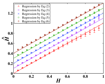
Figure 1: Comparison of the estimated Hurst index $\hat{H}$ using Eqs. (2-6) with the true value $H$. The error bars show the standard deviation of the 500 estimated $\hat{H}$ values. The results corresponding to Eqs. (3-6) are translated vertically for clarity.

In Fig. 2, we show the log-log plot of the detrended fluctuation $F(s)$ as a function of $s$ for two synthetic fractional Brownian surfaces with $H=0.2$ and $H=0.8$, respectively. There is no doubt that the power-law scaling between $F(s)$ and $s$ is very evident and sound. Hence, the two-dimensional DFA is able to well capture the self-similar nature of the fractional Brownian surfaces and results in precise estimation of the Hurst index.

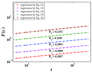
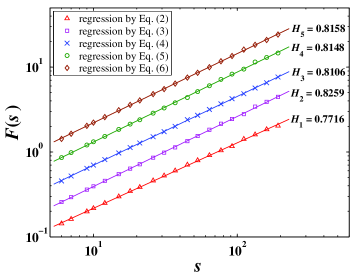
Figure 2: Log-log plots of the detrended fluctuation function $F(s)$ with respect to the scale $s$ for $H=0.2$ (top panel) and $H=0.8$ (bottom panel) using Eqs. (2-6). The lines are the least squares fits to the data. The results corresponding to Eqs. (3-6) are translated vertically for clarity.

We also adopted fractional Brownian surfaces to test the two-dimensional multifractal detrended fluctuation analysis. Specifically, we have simulated three fractional Brownian surfaces with Hurst indexes $H_{1}=0.2$, $H_{2}=0.5$, and $H_{3}=0.8$, respectively. The five regression equations (2-6) are used in the detrending. We calculated $h(q)$ for $q$ ranging from $-10$ to $10$ according to Eq. (13). All the $F_{q}(s)$ functions exhibit excellent power-law scaling with respect to the scale $s$. The function $\tau(q)$ can be determined according to Eq. (14). The resultant $\tau(q)$ functions are plotted in Fig. 3 with the inset showing the $h(q)$ functions. We can find from the figure that, for each surface, the five functions of $\tau(q)$ (and $h(q)$ as well) corresponding to the five detrending functions collapse on a single curve. Moreover, it is evident that $h(q)=H$ and $\tau(q)=qH-2$. The three analytic straight lines intersect at the same point $(q=0,\tau(q)=-2)$. These results are expected according to theoretical analysis.

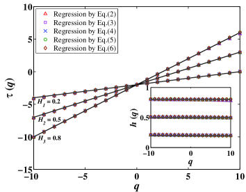
Figure 3: Plots of $\tau(q)$ extracted by using the five detrending functions (2-6) as a function of $q$. The three straight lines are $\tau(q)=qH-2$ for $H_{1}=0.2$, $H_{2}=0.5$, and $H_{3}=0.8$, respectively. The inset shows the corresponding $h(q)$ functions.

We stress that, when fractional Brownian surfaces are under investigation, both the two-dimensional DFA and MF-DFA can produce the same correct results even when Steps I-II are adopted.

III.2 Synthetic two-dimensional multifractals

Now we turn to test the MF-DFA method with synthetic two-dimensional multifractal measures. There exits several methods for the synthesis of two-dimensional multifractal measures or multifractal rough surfaces Decoster et al. (2000). The most classic method follows a multiplicative cascading process, which can be either deterministic or stochastic Mandelbrot (1974); Meneveau and Sreenivasan (1987); Novikov (1990); Meneveau and Sreenivasan (1991). The simplest one is the $p$-model proposed to mimick the kinetic energy dissipation field in fully developed turbulence Meneveau and Sreenivasan (1987). Starting from a square, one partitions it into four sub-squares of the same size and chooses randomly two of them to assign the measure of $p/2$ and the remaining two of $(1-p)/2$. This partitioning and redistribution process repeats and we obtain a singular measure $\mu$. A straightforward derivation following the partition function method Halsey et al. (1986) results in the analytic expression:

$$\tau(q)=q-1-\log_{2}\left[p^{q}+(1-p)^{q}\right]~{}.$$ (16)

A relevant method is the fractionally integrated singular cascade (FISC) method, which was proposed to model multifractal geophysical fields Schertzer and Lovejoy (1987) and turbulent fields Schertzer et al. (1997). The FISC method consists of a straightforward filtering in Fourier space via fractional integration of a singular multifractal measure generated with some multiplicative cascade process so that the multifractal measure is transformed into a smoother multifractal surface:

$$f(x)=\mu(x)\otimes|x|^{-(1-H)}~{},$$ (17)

where $\otimes$ is the convolution operator and $H\in(0,1)$ is the order of the fractional integration Decoster et al. (2000), whose $\tau(q)$ function is Arrault et al. (1997); Decoster et al. (2000):

$$\tau(q)=q(1+H)-1-\log_{2}\left[p^{q}+(1-p)^{q}\right]~{}.$$ (18)

The third one is called the random $\cal{W}$ cascade method which generates multifractal rough surfaces from random cascade process on separable wavelet orthogonal basis Decoster et al. (2000).

In our test, we adopted the first method for the synthesis of two-dimensional multifractal measure. Starting from a square, one partitions it into four sub-squares of the same size and assigns four given proportions of measure $p_{1}=0.05$, $p_{2}=0.15$, $p_{3}=0.20$, and $p_{4}=0.60$ to them. Then each sub-square is divided into four smaller squares and the measure is redistributed in the same way. This procedure is repeated 10 times and we generate multifractal “surfaces” of size $1024\times 1024$. The resultant $\tau(q)$ functions estimated from the two-dimensional MF-DFA method are plotted in Fig. 4, where the inset shows the $h(q)$ functions. We can find that the five functions of $\tau(q)$ (and $h(q)$ as well) corresponding to the five detrending functions collapse on a single curve, which is in excellent agreement with the theoretical formula:

$$\tau(q)=-\log_{2}\left(p_{1}^{q}+p_{2}^{q}+p_{3}^{q}+p_{4}^{q}\right)~{}.$$ (19)

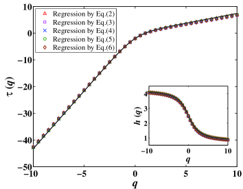
Figure 4: Plots of $\tau(q)$ extracted by using the five detrending functions (2-6) as a function of $q$. The continuous line is the theoretical formula (19). The inset shows the corresponding $h(q)$ functions.

We stress that, when we use Steps I-II instead of Steps 1-2, the resultant $\tau(q)$ estimated by the MF-DFA method deviates remarkably from the theoretical formula. Indeed, the power-law scaling for most $q$ values is absent and thus the alternative algorithm with Steps I-II and the resulting $\tau(q)$ is completely wrong. In addition, we see that different detrending functions give almost the same results. The linear function (2) is preferred in practice, since it requires the least computational time among the five.

IV Examples of image analysis

IV.1 The data

In this section we apply the generalized method to analyze two real images, as shown in Fig. 5. Both pictures are investigated by the MF-DFA approach since it contains automatically the DFA analysis. The first example is the landscape image of the Mars Yardangs region Alvarez-Ramirez et al. (2006), which can be found at http://sse.jpl.nasa.gov. The size of the landscale image is $2048\times 1536$ pixels. The second example is a typical scanning electron microscope (SEM) picture of the surface of a polyurethane sample foamed with supercritical carbon dioxide. The size of the foaming surface picture is $1200\times 800$ pixels.

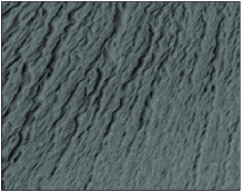
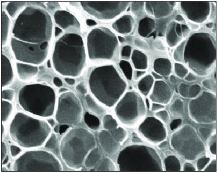
Figure 5: Left: The image of the Yardangs region on the Mars. Right: A scanning electron microscope picture of the surface of a polyurethane sample foamed with supercritical carbon dioxide.

The SEM picture of the surface of a polyurethane sample were prepared in an experiment of polymer foaming with supercritical carbon dioxide. At the beginning of the experiment, several prepared polyurethane samples were placed in a high-pressure vessel full of supercritical carbon dioxide at saturation temperature for gas sorption. After the samples were saturated with supercritical ${\rm{CO}}_{2}$, the carbon dioxide was quickly released from the high-pressure vessel. Then the foamed polyurethane samples were put into cool water to stabilize the structure cells. Pictures of the foamed samples were taken by a scanning electron microscope.

The two images were stored in the computer as two-dimensional arrays in 256 prey levels. We used Eq. (2) for the detrending procedure. The two-dimensional arrays were investigated by the multifractal detrended fluctuation analysis. For each picture, we obtained the $\tau(q)$ function and the $h(q)$ function as well. If $\tau(q)$ is nonlinear with respect to $q$ or, in other words, $h(q)$ is dependent of $q$, then the investigated picture has the nature of multifractality.

IV.2 Analyzing the Mars landscape image

We first analyze the Mars landscape image shown in the left panel of Fig. 5 with MF-DFA. Figure 6 illustrates the dependence of the detrended fluctuation $F_{q}(s)$ as a function of the scale $s$ for different values of $q$ marked with different symbols. The continuous curves are the best linear fits. The perfect collapse of the data points on the linear lines indicates the evident power law scaling between $F_{q}(s)$ and $s$, which means that the Mars landscape is self-similar.

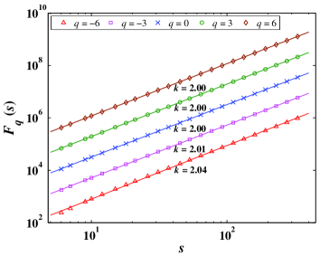
Figure 6: Log-log plots of the detrended fluctuation function $F_{q}(s)$ versus the lag scale $s$ for five different values of $q$. The continuous lines are the best fits to the data. The plots for $q=-3$, $q=0$, $q=3$, and $q=6$ are shifted upwards for clarity.

The slopes of the straight lines in Fig. 6 give the estimates of $h(q)$ and the function $\tau(q)$ can be calculated accordingly. In Fig. 7 is shown the dependence of $\tau(q)$ with respect to $q$ for $-6\leqslant{q}\leqslant 6$. We observe that $\tau(q)$ is linear with respect to $q$. This excellent linearity of $\tau(q)$ is consistent with the fact that $h(q)$ is almost independent of $q$, as shown in the inset. Hence, the Mars landscape image does not possess multifractal nature.

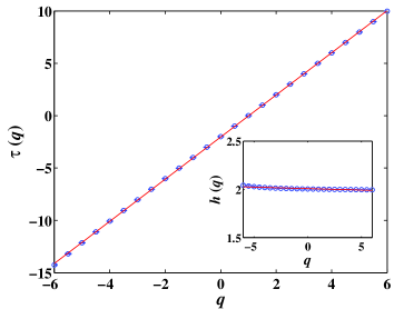
Figure 7: Dependence of $\tau(q)$ with respect to $q$. The solid line is the least squares fit to the data. The inset plots $h(q)$ as a function of $q$.

IV.3 Analyzing the foaming surface image

Similarly, we analyzed the foaming surface shown in the right panel of Fig. 5 with the MF-DFA method. Figure 8 illustrates the dependence of the detrended fluctuation $F_{q}(s)$ as a function of the scale $s$ for different values of $q$ marked with different symbols. The continuous curves are the best linear fits. The perfect collapse of the data points on the linear line indicates the evident power law scaling between $F_{q}(s)$ and $s$, which means that the Foaming surface is self-similar.

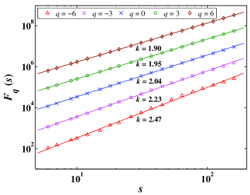
Figure 8: Loglog plots of the detrended fluctuation function $F_{q}(s)$ versus the lag scale $s$ for five different values of $q$. The continuous lines are the best fits to the data. The plots for $q=-3$, $q=0$, $q=3$, and $q=6$ are shifted upwards for clarity.

The values of $h(q)$ are estimated by the slopes of the straight lines illustrated in Fig. 8 for different values of $q$. The corresponding function $\tau(q)$ is determined according to Eq. (14). In Fig. 9 is illustrated $\tau(q)$ as a function of $q$ for $-6\leqslant{q}\leqslant 6$. We observe that $\tau(q)$ is nonlinear with respect to $q$, which is further confirmed by the fact that $h(q)$ is dependent of $q$, as shown in the inset. The nonlinearity of $\tau(q)$ and $h(q)$ shows that the foaming surface has multifractal nature.

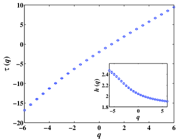
Figure 9: Dependence of $\tau(q)$ with respect to $q$. The inset shows $h(q)$ as a function of $q$.

V Discussion and conclusion

In summary, we have generalized the one-dimensional detrended fluctuation analysis and multifractal detrended fluctuation analysis to two-dimensional versions. Further generalization to higher dimensions is straightforward. We have found that the higher-dimensional DFA methods should be performed locally in the sense that the cumulative summation should be conducted after the partitioning of the higher-dimensional multifractal object. Extensive numerical simulations validate our generalization. The two-dimensional MF-DFA is applied to the analysis of the Mars landscape image and foaming surface image. The Mars landscape is found to be a fractal while the foaming surface exhibits multifractality.

At last, we would like to stress that there are tremendous potential applications of the generalized DFA in the analysis of fractals and multifractals. In the two-dimensional case, the methods can be adopted to the investigation of the roughness of fracture surfaces, landscapes, clouds, and many other images possessing self-similar properties. In the case of three dimensions, it could be utilized to qualify the multifractal nature of temperature fields and concentration fields. Possible examples in higher dimensions are stranger attractors in nonlinear dynamics. Concrete applications will be reported elsewhere in the future publications.