Dynamics and (de)localization in a one-dimensional tight-binding chain

Abstract

A simple tight-binding model is used to illustrate how the time dependence of a state vector can be obtained from all the eigenvalues and eigenvectors of the Hamiltonian. The behavior of the eigenvalues and eigenvectors is studied for various parameters and allows us to study scattering-like events, impurity states, and localization in disordered systems.

Published in Am. J. Phys. 74, 692 (2006).

I Introduction

For most physics students the Schrödinger representation of quantum mechanics is more appealing than the matrix or Heisenberg representation. The reason is due in part to the fact that the Schrödinger representation is more suited for visualization.goldb ; Schiff Also most students are more accustomed to thinking in terms of functions rather than in terms of abstract eigenvectors.

In this article I discuss a simple but versatile tight-binding Hamiltonian whose eigenvalues, eigenvectors and dynamics can be obtained and easily visualized in the matrix representation. The solution of the physical system represented by the Hamiltonian is obtained numerically by using a short program that is given in Appendix A. The code allows for visualization of the spectrum of eigenvalues and eigenvectors and also the dynamics generated by the Hamiltonian.

The model Hamiltonian of a one-dimensional chain with nearest neighbor couplings is discussed in Sec. II and a complete set of states describing the single particle dynamics is introduced. Section III briefly describes how the Hamiltonian generates the time dependence of an initial state vector and demonstrates that the eigenvalues and eigenvectors define the dynamical behavior of the system. In Sec. IV I discuss several applications that are of pedagogical interest. In particular, the dynamics of a state initially localized on a particular site is studied. The dynamics is correlated with the spectrum of the Hamiltonian and properties of its eigenvectors (localized versus delocalized). Several aspects of the problem that are of research interest are discussed, including the problems of localization and conductance in chain-like molecules, such as DNA.

II Definition of the problem

Consider the Hamiltonian:

$$H=\sum_{i}E_{i}c_{i}^{\dagger}c_{i}+\sum_{i}T_{i}[c_{i+1}^{\dagger}c_{i}+c_{i}^{\dagger}c_{i+1}],$$ (1)

where $c_{i}^{\dagger}$ and $c_{i}$ are the creation and destruction operators of a particle on site $i$, respectively. The Hamiltonian represents a chain of sites denoted by indices $i$; a particle can hop from one site to another due to the nonvanishing values of $T_{i}$ which are often called hopping matrix elements.

We restrict our attention to a single particle (or, more generally, an excitation) propagating through the chain. The dynamics can be described in a position-occupation basis, that a basis of states denoted by $\left\{|i\rangle,i=1,\ldots,N\right\}$ such that

$$|i\rangle=|00\ldots 1_{i}\ldots 0\rangle,$$ (2)

where $i$ denotes a particular site occupied by an excitation and $N$ denotes the total number of sites. The action of $c$-operators in this basis is simple:

$$c_{i}^{\dagger}|0\rangle =|i\rangle$$ (3a)

$$c_{i}|i\rangle =|0\rangle$$ (3b)

$$c_{i}|j\rangle =0,\quad i\neq j,$$ (3c)

where we consider only singly occupied states; the vacuum is denoted by $|0\rangle$. In the basis that is restricted to singly occupied states, we can equivalently (and without reference to creation/destruction operators) represent the Hamiltonian as

$$H=\sum_{i}E_{i}|i\rangle\langle i|+\sum_{i}T_{i}\big{[}|i+1\rangle\langle i|+|i\rangle\langle i+1|\big{]}.$$ (4)

The position-occupation basis does not diagonalize the Hamiltonian in Eq. (1), except in the trivial case of $T_{i}=0$ for all $i$. However, it is the basis that is simplest conceptually and most easy to visualize.

Equation (1) is a simplified tight-binding Hamiltonian and is discussed in many textbooks on condensed matter physics (see for example, Ref. Ashk, ). Its matrix representation is easy to construct. The simplest and numerically most feasible way is to consider a tridiagonal matrix in the position-occupation basis (Eqs. (2) and (3)) as

$$H=\begin{pmatrix}E_{1}&T_{1}&0&0&\cdots&0&0\cr T_{1}&E_{2}&T_{2}&0&\cdots&0&0\cr 0&T_{2}&E_{3}&T_{3}&\cdots&0&0\cr\vdots&\vdots&\vdots&\vdots&\ddots&\vdots&\vdots\cr 0&0&0&0&\cdots&E_{N-1}&T_{N-1}\cr 0&0&0&0&\cdots&T_{N-1}&E_{N}\end{pmatrix}.$$ (5)

The Hamiltonian is represented in a basis of singly occupied states; that is, we consider only this subset of states of Fock space (which includes multiply occupied states; for example, we might want to consider the dynamics of two excitations). Note that the Hamiltonian defined in Eq. (1) cannot induce transitions between the Fock subspaces corresponding to a different total number of excitations.

Periodic boundary conditions are not imposed in the matrix representation in Eq. (5). Periodic boundary conditions would require nonvanishing $(1,N)$ and $(N,1)$ elements, that is, the upper right and the lower left corner of the matrix. The matrix in Eq. (5) can be easily set up and diagonalized numerically. It is enough to specify only two arrays of real numbers, one of length $N$ which contains the diagonal values of the matrix, and the other of length $N-1$ which contains the elements of the Hamiltonian matrix along its first subdiagonal.

III Time dependence of state vectors

Let us assume that all the eigenvalues $\epsilon_{k}$ and eigenvectors $|\xi_{k}\rangle$ of the Hamiltonian $H$ are known ($H|\xi_{k}\rangle=\epsilon_{k}|\xi_{k}\rangle$). We further assume that the system is at time $t=0$, in some known or prepared state $|\Psi(t=0)\rangle$. The state $|\Psi(t=0)\rangle$ can be projected onto the basis of eigenvectors of the full Hamiltonian:

$$|\Psi(t=0)\rangle=\sum_{k}a_{k}|\xi_{k}\rangle,$$ (6)

where the projection coefficients $a_{k}$ are given by

$$a_{k}=\hskip 1.0pt\langle\xi_{k}|\Psi(t=0)\rangle,$$ (7)

because the $|\xi_{k}\rangle$ are assumed to be orthonormal, that is,

$$\hskip 1.0pt\langle\xi_{m}|\xi_{n}\rangle=\delta_{m,n}.$$ (8)

Let us denote the time evolution operator by $U(t)$; that is, $U(t)$ acts on an arbitrary state $|\Psi(t=0)\rangle$ and evolves it to the state $|\Psi(t)\rangle$,

$$U(t)|\Psi(t=0)\rangle=|\Psi(t)\rangle.$$ (9)

The action of the time evolution operator on the eigenvectors of the problem is trivialSchiff2 :

$$U(t)|\xi_{k}\rangle=\exp(-i\epsilon_{k}t/\hbar)|\xi_{k}\rangle,$$ (10)

which implies that

$$|\Psi(t)\rangle = \sum_{k}a_{k}\exp(-i\epsilon_{k}t/\hbar)|\xi_{k}\rangle$$ (11)

$$= \sum_{k}\langle\xi_{k}|\Psi(t=0)\rangle\exp(-i\epsilon_{k}t/\hbar)|\xi_{k}\rangle.$$ (12)

We assume that the wave function (or state vector) is initially chosen to be localized on a particular site $l$ of the chain, that is, $|\Psi(t=0)\rangle=|l\rangle$. We ask about the probability that after some time $t$ the excitation is on some other site $m$. To obtain this information, the state vector $|\Psi(t)\rangle$ must be projected onto the position-occupation basis, that is, we should calculate $N$ projections $b_{m,l}(t)$

$$b_{m,l}(t)=\langle m|\Psi(t)\rangle=\sum_{k}\hskip 1.0pt\langle\xi_{k}|l\rangle\hskip 2.84526pt\langle m|\xi_{k}\rangle\exp(-i\epsilon_{k}t/\hbar).$$ (13)

The quantity $|b_{m,l}(t)|^{2}$ is the probability that at time $t$, the excitation initially localized on site $l$ is found on site $m$. A pedagogical account of the definition of probability current in tight-binding problems can be found in Ref. Erasmo, .

IV Applications of the model

As mentioned, the matrix in Eq. (5) can be diagonalized numerically. One possible way of doing so is described in Appendix A, which lists a sample program to set up the Hamiltonian matrix and diagonalize it. The result of this numerical procedure is an array of $N$ Hamiltonian eigenvalues $\epsilon_{k}$ and a $N\times N$ matrix (or 2D array) of eigenvectors $|\xi_{k}\rangle$, which provides a complete solution of the problem, including its time dependence. In the following I present several applications of the code.

IV.1 Regular chain, propagation of the initially localized state

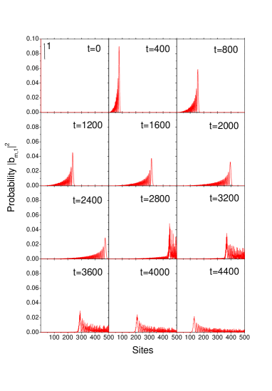
Figure 1: Time dependence of the probability distribution $|b_{m,1}|^{2}$ for a completely regular chain. The excitation was initially localized on the first site, that is, $|\Psi(t=0)\rangle=|1\rangle$. The time is measured in units of $\hbar/e$ and the number of sites $N=500$.

I first consider a completely regular chain, that is, a chain in which $E_{i}=E$ and $T_{i}=T$ for all $i$. The characteristic energies ($E$) and the hopping matrix elements ($T$) are set to $E=e$ and $T=-0.1e$, where $e$ denotes the energy scale. Note that the chosen energy scale also fixes the characteristic time scale, which is given by $\hbar/e$ (see Eq. (13)). The results of this calculation are given in Figs. 1 and 2. It is clearly observed how the initially localized state delocalizes over many sites and eventually hits the right end of the chain, reflecting from it. The horizontal axis in the plots is the site index which is in principle unrelated to any characteristic length. The spatial dimensions are hidden in the hopping (or overlap) matrix elements $T_{i}$; the more separated the atomic orbitals $E_{i}$ are, the smaller their overlap and the corresponding hopping matrix element.Ashk

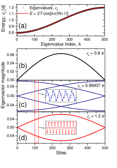
Figure 2: Eigenvalues and three characteristic eigenvectors of a regular chain. (a) Hamiltonian eigenvalues, (b) eigenvector of the lowest energy eigenstate ($\epsilon_{k}=0.8e$), (c) eigenvector of eigenstate with energy $\epsilon_{k}=0.99937e$ (250th eigenstate), and (d) eigenvector of eigenstate with energy $\epsilon_{k}=1.2e$ (highest energy eigenstate). The insets in the (c) and (d) show the eigenvector magnitude between the 100th and 120th sites (these are blowups of the eigenvector magnitude in the regions bounded by the two thin rectangles in the main plots).

Figure 2 displays the eigenvalues of the Hamiltonian and three characteristic eigenvectors. Note the fast oscillatory behavior of the eigenvectors for high-energy states (insets in (c) and (d) panels of Fig. 2). The eigenvalues of the Hamiltonian are indistinguishable from the analytical solution, which is given by Boykin

$$\epsilon_{k}=E+2T\cos[k\pi/(N+1)],$$ (14)

where $k$ is the eigenvalue index ($k=1,\ldots,N$), that is, a cosine band of states of width $W\approx 4T=0.4e$. The exact solution for the periodic tight-binding chain isAshk

$$\epsilon(k)=E+2T\cos(2k\pi/N),\qquad(k=1,\ldots,N)$$ (15)

Note the extra factor of $2$ in the argument of the cosine compared to Eq. (14) and that the eigenvalue $\epsilon_{k}$ has been rewritten as $\epsilon(k)$, so that it appears as a function of the eigenvalue index. In the periodic case, it makes sense to characterize the eigenvalues by the wavevector, that is, $k$ becomes more than an eigenvalue index and has a direct interpretation in terms of the characteristic wavelength for each eigenstate. This issue is discussed in more detail in Appendix B.

Note that Eqs. (14) and (15) are not very different for large $N$. In the limit of infinite $N$, the band width, defined as the difference between the largest and smallest eigenvalues, is the same in both cases, as well as the density of states defined as

$$\rho(\epsilon)=\sum_{k}\delta(\epsilon-\epsilon_{k}).$$ (16)

There is one important difference, that is, the double degeneracy of states given by Eq. (15) for states with $k_{1}=l$ and $k_{2}=N-l$, $l=1,\ldots,N-1$, which is not the case in Eq. (14).

IV.2 One defect link in a chain, simulation of scattering

In this subsection, a special link is introduced between the 250th and 251st sites in a chain with total of $N=500$ sites so that $T_{250}=-0.2e$, and all other links are the same as before, $T_{i}=-0.1e$ for all $i$, $i\neq 250$ (the orbital energies are $E_{i}=e$ for all $i$, the same as in previous subsection). This modification of the hopping matrix will allow us to study the effects of the impurity link on the eigenvalue spectrum and propagation of the initially localized state.

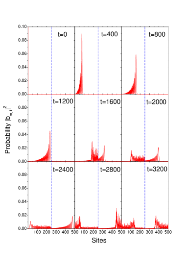
Figure 3: Time dependence of the probability distribution for a regular chain with a special link inserted between the 250th and the 251st site of the chain (denoted by dashed lines in the plots). The time is measured in $\hbar/e$.

The evolution of a state vector initially localized on the first chain site is displayed in Fig. 3. Note how part of the probability density is reflected from site 250 and 251, while the other part continues its propagation toward the end of the chain.

The eigenvalue spectrum is shown in Fig. 4. Note the appearance of two states that detach from the band. The eigenvectors of two special states are also displayed in Fig. 4. The two states separated from the band correspond to the excitations that are localized on the special sites 250 and 251, that is, these states are related to excitations of impurity sites.

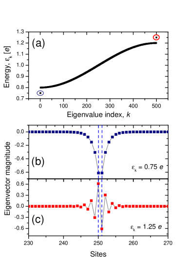
Figure 4: Eigenvalues and the two eigenvectors corresponding to impurity excitation states. (a) Hamiltonian eigenvalues, (b) eigenvector of the lowest energy eigenstate ($\epsilon_{k}=0.75e$), and (c) eigenvector of highest energy ($\epsilon_{k}=1.25e$). The two sites that are connected with an impurity link are denoted by dashed lines in (b) and (c).

IV.3 Anderson’s diagonal disorder Hamiltonian

We now study a case in which randomness is introduced in the Hamiltonian matrix. The orbital energies $E_{i}$ are given random values in a band of width $W$. Because these numbers are along the diagonal of the Hamiltonian, the model is said to have diagonal disorder. The sub-diagonal matrix elements are the same as before ($T_{i}=T=-0.1e$). There are a number of interesting issues related to this model, one of which is called Anderson localization. The suitably modified code in Appendix A can be used to study the Anderson’s diagonal disorder Hamiltonian. The number of sites is increased to $N=900$ and the orbital energies along the diagonal are given uniform random values in the interval $[e,2e]$, that is, $W=e$.

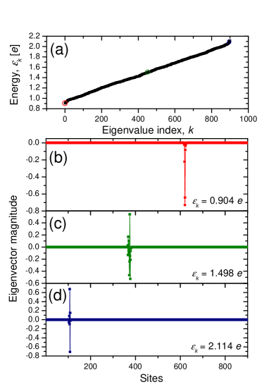
Figure 5: Eigenenergies and three characteristic eigenvectors of the Anderson’s diagonal disorder Hamiltonian.

One of the features of this problem is that all the eigenstates of the Hamiltonian are localized.Anders1 ; Anders2 The eigenvalue spectrum and three characteristic eigenvectors are shown in Fig. 5. The fact that all the eigenvectors are localized has a profound influence on the propagation of an initially localized state. Figure 6 displays an evolution of a state vector initially localized on the first chain site. Occupation probabilities for the first 30 sites of the chain are presented; the site occupation probabilities are negligible beyond site 10. Note that the times shown are very long ($t=10^{16}\hbar/e$). We conclude that the propagation of the excitation through the chain is not only slow, but is effectively blocked – the excitation remains localized in the vicinity of the site at which it was initially created.Anders1 ; Anders2 The blockage of the excitation propagation is related to the fact that the projection coefficients ($a_{k}$ in Eq. (6)) of the initially localized state have a significant magnitude only for several eigenstates whose localization on the first site is nonvanishing. One of those eigenvectors (the one whose maximum magnitude is on the first site) is very similar to the initial state vector, and its projection coefficient is the largest and close to 1. Thus, the initial state is almost an eigenstate and its evolution is thus slow. Because the projection coefficients $a_{k}$ on eigenvectors that are localized on sites that are very distant from the first chain site are close to zero, the propagation through the chain is essentially blocked. The total number of the sites that become occupied during the evolution (about 5 to 10 as is seen in Fig. 6) is related to the typical localization width of the eigenvectors.

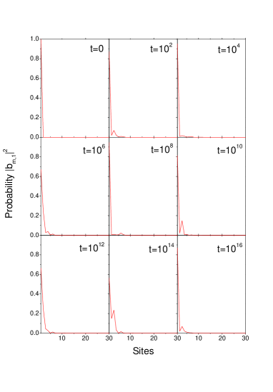
Figure 6: Time dependence of the probability distribution for a chain with random orbital energies chosen from the interval $[e,2e]$. The time is measured in $\hbar/e$. Note that only the first 30 sites of the chain with 900 sites are represented, because the site occupation probabilities are negligible beyond the 10th site.

IV.4 Recent research on chains in the tight-binding scheme

It is interesting to see how the possible correlations in the diagonal disorder distribution influence the nature of the eigenvectors and the spectrum of eigenvalues (see for example, Refs. corrdis, and corrdis2, ). These effects could be studied with suitable changes of the code. The localization of electronic states due to disorder may drive a metal-insulator transition (or Anderson transition) in the system, and one-dimensional models similar to the one discussed in this article are useful in the study of random binary alloys.Naturer In this case there are only two characteristic orbital energies and their appearance in the chain is random (for example, the appearance of the A orbital occurs with probability $p$, while the appearance of the B orbital occurs with probability $1-p$). For a random binary alloy, the system again exhibit the localization of eigenvectors, but correlations in the disorder may introduce resonant states for which there is perfect electron transmission through the system.

The electrical conduction of biological polymers, DNA in particular, has also attracted much attention.Naturer ; DNAcond An electronic coupling induced through the overlap of $\pi_{z}$ orbitals perpendicular to the planes of the stacked base pairs in double-stranded DNA can be simulated using the simplified one-dimensional model in Eq. (1), although the realistic situation is much more complicated due to the influence of vibrations on the distances between the base pairs and the importance of the electronic structure of the DNA backbone. DNAcond ; Bruinsma1 ; Dekker1 ; stretch Models similar to the one studied in this article are used to study the conduction properties of DNA molecules.Naturer

The model and the program in Appendix A can be easily modified to study these problems. Correlations in the diagonal disorder can be studied, as well as the introduction of disorder along the sub-diagonals (hopping matrix elements). Localization effects can be studied in cases when the width of the diagonal energy band $W$ is much smaller than the value of the hopping matrix elements $T$. The opposite limit was studied in Sec. IV.3.

Appendix A A program for the study of the problem

The following code describes the numerical solution to the problem. Due to the brevity of the code, it is listed here along with comments. The source code can be compiled as g77 -o chain1 chain1.for -llapack or f77 -o chain1 chain1.for -llapack
depending on the Fortran compiler installed. Note that the code should be linked to the LAPACK library of routines lapack .

1     program tba1d
2     double precision E(5000), T(5000), XI(5000,5000),
     &       flag, work(9998), thresh, time, ReB, ImB
3     open(1, file=’eigenvalues.dat’, status=’unknown’)
4     open(2, file=’eigenvectors.dat’, status=’unknown’)
5     N = 500
* Number of chain sites
6     thresh = 0.0D0
* Threshold for random function
7     do i=1, N
8      E(i) = 1.0
* E - diagonal of hamiltonian matrix - orbital
9      flag = rand()
10     T(i) = -0.1
* T - subdiagonal of hamiltonian matrix - hopping
11     if (flag .lt. thresh) then
12      E(i) = 1.0 + 1.0*rand()
13     endif
14    enddo
15    call DSTEV(’V’,N,E,T,XI,5000,work,info)
16    do i=1, N
17     write(1,*) i, ’ ’,  E(i)
* On exit from DSTEV, E contains eigenvalues
18     write(2,*) ’Eigenvector: ’, i
19      do j=1, N
20       write(2,*) XI(j,i)
* On exit from DSTEV, XI contains eigenvectors
21      enddo
22    enddo
23    close(1)
24    close(2)
25    l = 1
* Index of initially occupied site
26    print *,’Input: time t’
27    read *, time
28    open(4, file=’timedat.dat’, status=’unknown’)
29    do j=1, N
* j counts the chain sites
30     ReB = 0.0D0
31     ImB = 0.0D0
* Real and imaginary parts
32     do i=1, N
* i counts the eigenstates
33      ReB = ReB + XI(l,i)*dcos(E(i)*time)*XI(j,i)
34      ImB = ImB - XI(l,i)*dsin(E(i)*time)*XI(j,i)
35     enddo
36     write(4,*) j, ’ ’, ReB**2 + ImB**2
37    enddo
38    close(4)
39    end

The total number of sites in a chain ($N$) is defined in line 5. The Hamiltonian matrix is defined between lines 7 and 14. The parameter thresh allows for the introduction of random orbital matrix elements (lines 11–13); for thresh = 0 the orbitals are regular, while for thresh > 1 they are totally random within the ranges defined by line 12 (between 1 and 2 energy units).

The Hamiltonian matrix is diagonalized in line 15 using the DSTEV LAPACK routine designed for the diagonalization of tridiagonal matrices.lapack After the diagonalization, the $j$th column of the matrix XI(i,j) contains the eigenvector corresponding to the $j$th eigenvalue of the Hamiltonian ($|\xi_{j}\rangle$). The DSTEV routine sorts the eigenvalues in an ascending order.

The time dependence of the initial state vector, one of the vectors from the $\{|i\rangle\}$ basis in Eq. (2), is implemented between lines 25 and 37. In particular, the part of the program between lines 29 and 37 implements Eq. (13). The initial state is specified by the variable l which represents the index of the occupied chain site at $t=0$.

The output is written in the file timedat.dat which can be plotted separately. This output was used to generate Figs. 1, 3, and 6. The CPU time needed to calculate the probability distribution does not depend on the physical time input (variable time) because the program does not propagate a solution in the time domain. All the calculations needed for the evolution of the initial state vector are performed by the diagonalization of the Hamiltonian matrix. This output is used to calculate the probability distributions for arbitrary times $t$ (see Eq. (13)).

To implement the case of regular chain discused in subsection IV.1, all randomness must be eliminated, and thus, the thresh variable in line 6 is set to zero.

To simulate one special link (impurity or defect) in the middle of the chain with $N=500$ sites (the case studied in subsection IV.2), we introduce the following piece of code in between the lines 13 and 14,

if (i .eq. 250) then
 T(i) = -0.2
endif

The rest of the lattice is in a regular state, that is, line 6 which controls the amount of randomness in the chains is still

thresh = 0.0D0

For the case of totally disordered chain with $N=900$ sites studied in subsection IV.3, lines 5 and 6 of the code should be changed to

5     N = 900
6     thresh = 1.0D0

Appendix B Periodic version of the regular tight-binding chain

To obtain a chain that is periodic, we have to connect the first and the $N$th sites by the hopping matrix elements. Hence, the Hamiltonian matrix is no longer tridiagonal because it now contains nonvanishing $(1,N)$ and $(N,1)$ elements. However, the Hamiltonian matrix is still symmetric. The periodic chain is easily programmed using techniques similar to those described in Appendix A (the code can be obtained from the author). For the periodic case the upper (or lower) triangle of the Hamiltonian matrix and not only its diagonal and main subdiagonal has to be stored.

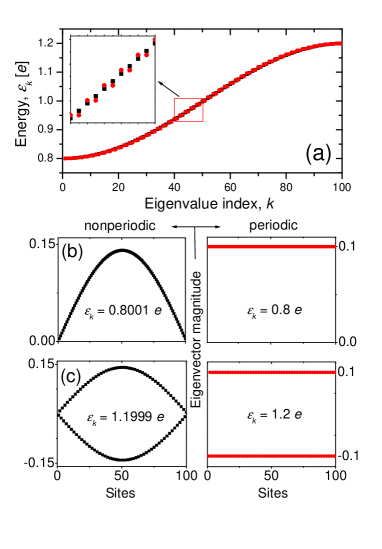
Figure 7: Comparison of the eigenvalues and two characteristic eigenvectors for a uniform chain with non-periodic (squares) and periodic (circles) boundary conditions. The parameters are $E=e$, $T=-0.1e$, and $N=100$. (a) Eigenvalues of non-periodic and periodic chain, (b) eigenvectors of the lowest energy eigenstates, and (c) eigenvectors of the highest energy eigenstates.

The results for a regular periodic chain are shown in Fig. 7 and compared with the case studied in Sec. IV.1. The parameters of the calculation are $E=e$, $T=-0.1e$, and $N=100$. The results are used to illustrate subtleties discussed at the end of Sec. IV.1. Note that the eigenvalue spectra look indistinguishable, but a closer inspection (inset in Fig. 7(a)) reveals that the spectrum corresponding to the periodic chain is doubly degenerate (except for the lowest and highest energy eigenvalue), which is not the case for the nonperiodic chain, in agreement with the discussion in Sec. IV.1. The eigenvectors corresponding to the lowest and highest energy eigenstate are also different (which is true for all eigenvectors) although the energies of these states are similar in the two cases, see Eqs. (14) and (15)). For the periodic chain the lowest energy eigenvector can be written in the position-occupation basis as

$$|\xi_{\rm lowest}\rangle=\frac{1}{\sqrt{N}}|1,1,1,1\ldots 1\rangle,$$ (17)

and the highest energy eigenvector in the same basis is

$$|\xi_{\rm highest}\rangle=\frac{1}{\sqrt{N}}|-1,1,-1,1\ldots 1\rangle.$$ (18)

References

- (1) A very good example is the article by A. Goldberg, H. M. Schey, and J. L. Schwartz, “Computer-generated motion pictures of one-dimensional quantum-mechanical transmission and reflection phenomena,” Am. J. Phys. 35 (3), 177–186 (1967).
- (2) Leonard I. Schiff, Quantum Mechanics (McGraw-Hill, Singapore, 1968), 3rd ed., pp. 106–109.
- (3) Neil W. Ashcroft and N. David Mermin, Solid State Physics (Saunders College Publishing, Fort Worth, 1976), college ed., pp. 176–190
- (4) Leonard I. Schiff, Quantum Mechanics (McGraw-Hill, Singapore, 1968), 3rd ed., pp 53.
- (5) Erasmo A. de Andrada e Silva, “Probability current in the tight-binding model,” Am. J. Phys. 60 (8), 753–754 (1992).
- (6) Timothy B. Boykin and Gerhard Klimeck, “The discretized Schrödinger equation and simple models for semiconductor quantum wells” Eur. J. Phys. 25 (4), 503–514 (2004).
- (7) P. W. Anderson, “Localized moments and localized states,” Rev. Mod. Phys. 50 (2), 191–201 (1978).
- (8) P. W. Anderson, “Absence of diffusion in certain random lattices,” Phys. Rev. 109 (5), 1492–1505 (1958).
- (9) Francisco A. B. F. de Moura and Marcelo L. Lyra, “Delocalization in the 1D Anderson model with long-range correlated disorder,” Phys. Rev. Lett. 81 (17), 3735–3738 (1998).
- (10) Hiroaki Yamada, “Localization of electronic states in a nonstationary chaotic field with long-range correlation,” Phys. Rev. B 69 (1), 014205-1–8 (2004).
- (11) Pedro Carpena, Pedro Bernaola-Galván, Plamen Ch. Ivanov, and H. Eugene Stanley, “Metal-insulator transition in chain with correlated disorder,” Nature 418, 955–959 (2002).
- (12) R. G. Endres, D. L. Cox, and R. R. P. Singh, “The quest for high-conductance DNA,” Rev. Mod. Phys. 76 (1), 195–214 (2004).
- (13) R. Bruinsma, G. Grüner, M. R. D’Orsogna, and J. Rudnick, “Fluctuation-facilitated charge migration along DNA,” Phys. Rev. Lett. 85 (20), 4393–4396 (2000).
- (14) Gianaurelio Cuniberti, Luis Craco, Danny Porath, and Cees Dekker, “Backbone-induced semiconducting behavior in short DNA wires,” Phys. Rev. Lett. 65, 241314-1–4 (2002).
- (15) Paul Maragakis, Ryan Lee Barnett, Efthimios Kaxiras, Marcus Elstner, and Thomas Frauenheim, “Electronic structure of overstretched DNA,” Phys. Rev. B 66, 241104-1–4 (2002).
- (16) E. Anderson, Z. Bai, C. Bischof, J. Demmel, J. Dongarra, J. DuCroz, A. Greenbaum, S. Hammarling, A. McKenney, and D. Sorensen, LAPACK User’s Guide (SIAM Publications, Philadelphia, PA, 1999), 3rd ed., For more information, see <www.netlib.org/lapack/>.