An indicator for community structure

Abstract

An indicator for presence of community structure in networks is suggested. It allows one to check whether such structures can exist, in principle, in any particular network, without a need to apply computationally cost algorithms. In this way we exclude a large class of networks that do not possess any community structure.

Introduction

Community structure of networks have been intensively studied in recent years, and a number of algorithms for finding such structures have been suggested Newman-Girvan ; review . Being quite effective, these algorithms allow one to find the community structure in a wide variety of networks. However, such algorithms are quite complicated and computationally demanding, moreover not all networks possess any community structure at all. Therefore it seems desirable to have some simple enough indicator allowing one to judge about potential existence of community structures in networks prior to exploiting the algorithms for finding them. The usage of such an indicator could be quite effective in negative sense, i.e. the negative answer to the question whether a particular network can have any community structure or not would allow one to exclude such a network from consideration, thus avoiding a use of complicated numerical procedures for community structure evaluation.

In this paper we propose an indicator of existence of community structure in networks, which is based on a geometrically motivated measure that compares an average network distance with its ”mean diameter”. The indicator is oriented on relatively dense communities, which is typical for sociological type of networks social . We provide some asymptotic estimations for this indicator which allow one to evaluate its numerical values. The indicator is applied to some model networks with dense communities. Some real networks are analyzed as well.

Dilatation of a network as an indicator for community structure

Our goal is to find relatively simple indicator for community structure existence. The idea is to compare the mean distance, which can be easily calculated, with some etalon characteristic of networks of a given size $N$ and a mean degree $k$. To define such an etalon let us look at some geometric analogy. Consider an $n$-dimensional geometric body of volume $V$. In geometry the ratio between the diameter of the body to its minimal possible value (which is of order of $\sqrt[n]{V}$) is known as a dilatation Rickman , which is a measure of body’s asymmetry.

We adopt this concept to networks using the notion of a mean distance $\bar{L}$ instead of the diameter. First, notice that the size $N$ of a network can serve as an analog of geometric volume, and the ratio $\delta$ of the number of links to the number of nodes $N$ can be chosen as an analog of dimension. For undirected networks considered here, the dimension analog is $\delta=k/2$, where $k$ is the mean degree. For instance, the mean degree of a 2D-torus is $k=4$, for 3D-torus $k=6$, etc.

We introduce a notion of dilatation of a network and define it as

$$D=\frac{\bar{L}}{\sqrt[\delta]{N}}.$$ (1)

Intuitively, a large value of dilatation can be caused by strong inhomogeneity, which in turn can be a consequence of the presence of community structure in the network. However, the presence of community structure is just one of possible reasons for high network dilatation. For instance, highly stretched networks, such as a narrow long strip, can also have high value of dilatation. Therefore the dilatation can only indicate to possible existence of a community structure. In other words, big value of dilatation can serve as a necessary, but not sufficient condition for community structure existence.

To illustrate the relationship between community structure and dilatation consider a simplest possible configuration having an evident community structure, namely, a network consisting of two complete graphs of size $N/2$ each connected by a single link to each other. This network contains two communities of maximal density with a single inter-community link. For large networks ($N\gg 1)$ the mean distance and the dimension are $\bar{L}\approx 2$ and $\delta\approx N/4$, respectively, so the dilatation is (see Appendix for details)

$$D\approx\frac{2}{\sqrt[N/4]{N}}\rightarrow 2.$$ (2)

As another extreme example consider a network without any community structure, namely a binary tree of $M$ levels. The network size is $N=2^{M+1}-1$, the total number of links equals to $N-1$, so the dimension $\delta\approx 1$, and the mean distance can be estimated as $L\approx 2M$. Substituting $L$ and $\delta$ into Eq.(1) results in the following asymptotic expression for dilatation:

$$D\approx\frac{log_{2}N}{N}\rightarrow 0.$$ (3)

The described extreme examples prompt us to make a plausible conjecture that, in general, the dilatation of networks baring no community structure should be relatively small (less than one), whereas the dilatation of well-structured networks should be at least around 2. Below the last statement will be corrected based on both analytical estimations and further examples.

Asymptotical estimations

To develop analytical estimates we need to describe more formally community networks. Consider a global connected network $G$ comprising of $N$ nodes and $E$ links, so that the dimension of $G$ is $\delta=E/N$. To estimate the dilatation we need, according to Eq.(1), an estimation for the mean distance $\bar{L}_{G}$. To calculate $\bar{L}_{G}$ suppose that the network is divided into $C$ communities, so that $i-th$ community contains $m_{i}$ nodes. Let us also assume that any two communities are connected by a single link at maximum. It should be noted that being obtained under this assumption, our analytical estimations work quite well also beyond it, as will be demonstrated below. Let us define a macro network $M$ by replacing each of $C$ communities with a single node and denote the mean distance in $M$ by $\bar{L}_{M}$. The formulas for the dilatation and the mean distance in general case, derived in Appendix, assume some apriory knowledge about the structure of the network. It is possible however to get, under some additional assumptions, analytical estimations which do not demand any apriory knowledge about the structure of the network. Indeed, assuming that all communities have the same size $m_{i}=m\gg 1$ and the same mean distance $\bar{L}_{C}$, we obtain the following estimation for the mean distance $\bar{L}_{G}$ of the global network

$$\overline{L}_{G}\approx\left[\frac{1}{C}+\frac{2(C-1)}{C}\right]\overline{L}_{C}+\frac{C-1}{C}\overline{L}_{M},$$ (4)

where $\overline{L}_{C}$ is the mean distance inside a single community. Equation (4) still bears some apriory information about the community structure, namely the number of communities $C$ and the mean distance $\overline{L}_{C}$ inside a single community. Assuming that the number of communities is large enough $C\gg 1$ and taking into account that $\bar{L}_{C}\geq 1$ (equality takes place for a complete graph), results in

$$\overline{L}_{G}\geq\overline{L}_{M}+2.$$ (5)

Inequality (5) means that given a particular network with the mean distance $\overline{L}_{G}$, any reasonable partition of the network into dense communities will result in a macro network whose mean distance is not bigger than $\overline{L}_{G}-2$. If, on the other hand, after partitioning the network inequality (5) is violated, then the partition was not suitable. Notice that equality in (5) takes place when all communities are complete graphs (1-cliques social ).

Using Eq.(4) results in the following estimation for dilatation:

$$D\approx N^{-1/\delta}\left(\left[\frac{1}{C}+\frac{2(C-1)}{C}\right]\overline{L}_{C}+\frac{C-1}{C}\overline{L}_{M}\right).$$ (6)

Taking into account that $C\geq 2$, $\bar{L}_{C}\geq 1$ and $\bar{L}_{M}\geq 1$ (equality takes place for a complete graph) we obtain from Eq.(6) the following rough estimate which does not depend on any apriory knowledge about the community structure:

$$D\geq\frac{2}{\sqrt[\delta]{N}}.$$ (7)

For the case $C\gg 1$ it follows from Eqs.(5) and (6) that

$$D\geq\frac{\overline{L}_{M}+2}{\sqrt[\delta]{N}}\geq\frac{3}{\sqrt[\delta]{N}}.$$ (8)

Thus the behavior of the dilatation depends on the parameter $N^{1/\delta}=N^{N/E}$ that we call a mean diameter of the network.

This study is focused on Sparse networks with Dense communities (SD-networks), in which the value of $N^{1/\delta}$ is close to unity. We propose the following formal definition of SD-networks: A network $G$ is an SD-network if $\sqrt[\delta]{N}\rightarrow 1$ for $N\rightarrow\infty$. To satisfy this condition it is enough that the dependence of $\delta=E/N$ upon $N$ has the form of $E\geq N^{s}$ for $s>1$. As it follows from the above definition, for any large ($N\gg 1$) SD-network $D\geq 2$, where the estimation (5) was used. We remind that according to eq.(2) for the network consisting of two complete graphs of size $N/2$ connected by a single link the dilatation $D\approx 2/\sqrt[N/4]{N}\rightarrow 2$.

It should be noted that the asymptotic estimation $D\geq 2$ was obtained under additional restrictions on networks, namely: (i) all communities are large enough and have approximately the same size, (ii) all communities have the same mean distance, and (iii) there exists not more then one link between two different communities. However, in real-life networks these restrictions can be violated, therefore we suggest to use $D>1$ as a criterium for community structure existence. Numerical simulations presented in the next section support the choice of the criterium $D>1$.

Model examples

In this section we demonstrate, using numerical simulations, how the introduced above indicator of existence of community structure works on some model networks. It will be shown that the criterium $D>1$ is quite reasonable, even for relatively small communities. Also, it will be demonstrated that being derived in asymptotical limit $m\gg 1,C\gg 1$, analytical estimations Eqs.(5) and (7) are not restricted by this limit, and work quite well even for relatively small values of $m$ and $C$.

As a first model example consider a ring network with $n=20$ and $k=2$, in which each of all 20 nodes is replaced with a complete graph of size $m$. Two quantities have been calculated, the dilatation $D$, and the mean distance $\overline{L}_{G}$ as functions of $m$. The result is shown in Fig. 1. One can see that the for initial simple ring with $m=1$, that has no any structure, the dilatation is small. While the community size $m$ increases, the dilatation grows and exceeds 1 at $m>5$, when the community structure becomes clearly pronounced. One can also notice that starting from $m\leq 10$ the analytical estimations Eqs.(5) and (7) hold well. The same comment holds true for the lattice network (see Fig.2).

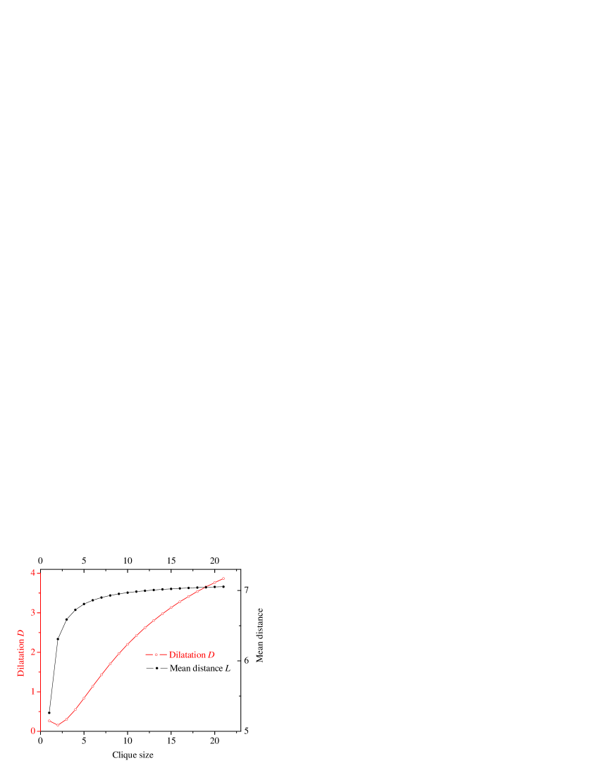
Figure 1: Ring network consisting of 20 complete-graph-clusters, $k=2$. Dependence of dilatation mean distance upon cluster size.

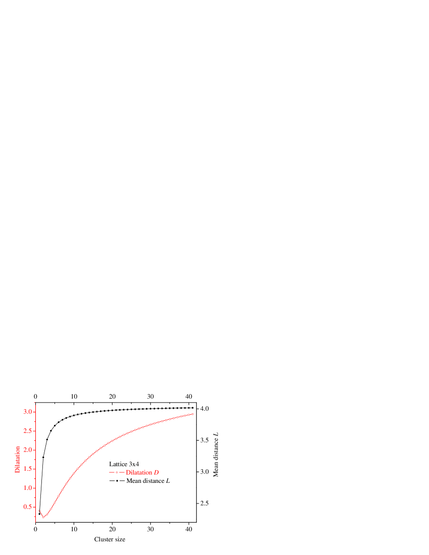
Figure 2: 3x4 lattice. Dependence of dilatation and the mean distance on cluster size.

Both the analytical estimations Eqs.(5) and (7) and the results shown in Figs. 1 and 2, have been obtained under assumption that all communities are of the same size. However, applicability of the estimations Eqs.(5) and (7) is not restricted to this assumption. To demonstrate this, we have constructed a network with variable community size, namely 4x3 lattice with community sizes randomly chosen between 20 and 60, so that the mean community size equals to 40. Calculation of the mean distance and the dilatation of this network gives $D=2.98\pm 0.07$ and $L=3.98\pm 0.06$. The same network with equal community sizes corresponds to the last point in Fig.2 where the dilatation and the mean distance are $D=2.92782$ and $L=4.01601$, correspondingly. Comparing the dilatation and the mean distance for these two networks one can conclude that the estimations Eqs.(5) and (7) work well for networks with not equal communities as well.

Consider again the 4x3 lattice network with equal communities, but now the communities are not complete graphs, namely each pair of nodes inside the communities is linked with probability $P$ called community density. So the number of inside-community links varies. The dilatation and the mean distance as functions of the community density $P$ is shown in Fig.3.

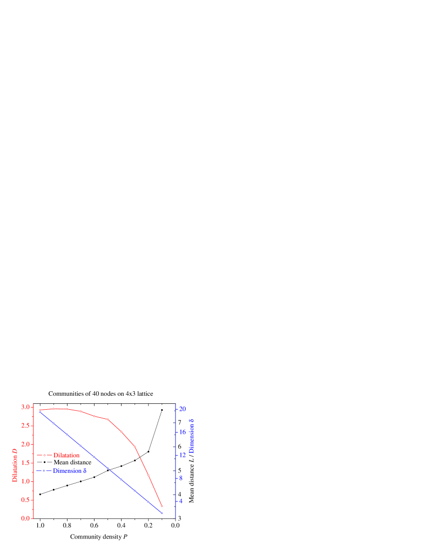
Figure 3: 3x4 lattice. Dependence of dilatation and the mean distance on the number of inside-community links.

As it can be seen from Fig.3, the dilatation keeps above unity even at quite low community density ($P>0.2$), indicating to existense of community structure. Moreover, the estimations Eqs.(5) and (7) work quite well, as long as the density of communities is not too low. At low values of $P<0.2$ the dilatation is less than 1 indicating to the absence of dense communities. This is consistent with the fact that the network dimension becomes low as well. We note again that both our indicator and analytical estimations are applicable to SD-networks (relatively dense communities sparsely connected to each other).

Another assumption made in the course of derivation of analytical estimations Eqs.(5) and (7) is that each pair of communities is connected by not more than one link. To check what happens when we go beyond this assumption, consider a network comprising of 5 randomly connected complete graphs, with the number of inter-community links increased gradually from the minimal value of 4 to the maximum of about 4000. Figure 4 shows the dependence of the mean distance and of the dilatation upon the number of inter-community links. As one can see, the dilatation remains above 1 up to quite large number of inter-community links (about 2000), afterwards different communities become overlapped, so that the border between communities cannot be defined clearly enough. At the point when the number of inter-community links reaches its maximum (4000) and $\delta=50$, the entire network becomes a complete graph, so that the mean distance equals to 1 and the dilatation is about 0.91. This value of dilatation differs from asymptotical one for complete graph due to the fact that the asymptotic $\sqrt[\delta]{N}\rightarrow 1$ is quite slow with respect to $\delta$, therefore $\sqrt[50]{N}=1.096$.

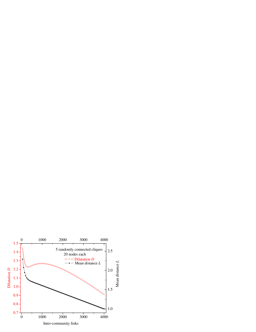
Figure 4: 5 randomly connected cliques, 20 nodes each. Dependence of the dilatation and the mean distance upon the number of inter-community links.

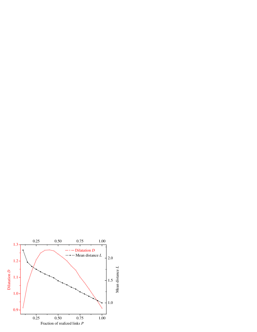
Figure 5: Random graph of 100 nodes. Dilatation and mean distance as functions of graph connectivity $P$.

Random graph

Recently Guimerá et al. Guimera have pointed out that Rene-Erdos random graph Erdos can exhibit a community structure due to fluctuations. Their observation was based on a concept of modularity introduced in Ref.Newman-Girvan . In this context it seems interesting to analyze such random graphs from the point of view of dilatation. To do this we have constructed a random graph containing 100 nodes connected to each other with probability $P$, and calculated its dilatation. In Fig. 5 both the dilatation and the mean distance are plotted as functions of $P$. One can notice a clear maximum at $P=0.4$ where the dilatation, $D\approx 2.4$. According to our concept this high value of dilatation indicates to possible existence of a community structure in the network. This conclusion is consistent with high modularity of random graphs reported in Ref. Guimera . It also seems that this can be related to another observation about possible hierarchy structure in random graphs our-hierarchy .

Real-life networks

To check how our indicator of the existence of community structures works for real-life networks, we have calculated the dilatation for 13 undirected networks using the data presented in the Table II from Ref. Newman-SIAM . The highest value of dilatation $D=2.766$ was obtained for the network of film actors actors , which indicates that this network should be well structured. Three other networks, train roots trainRouts , Internet Internet , and company directors CompanyDirectors , can also have community structure according to their dilatation values of 1.78, 1.48, and 1.33, respectively. All other networks presented in the table II from Ref. Newman-SIAM have the dilatation less than 1, therefore according to criterium $D>1$ they hardly can have a community structure. However, one should be careful using this criterium and keep in mind the assumptions under which it was obtained. For instance, looking at the data presented in the above mentioned table we notice that despite the fact that some networks, like math coauthorship, peer-to-peer and some other networks, have low dilatation, they are not dense enough (not SD-networks) to apply our criterium.

Summary

The notion of dilatation of networks has been introduced. Analytical estimations for the dilatation have been obtained under some reasonable assumptions. The value of dilatation is suggested to use as an indicator of existence of community structure in Sparse networks with Dense communities (SD-networks). Both some model and real-life networks have been considered to illustrate the usage of the indicator suggested, as well as the applicability of the analytical estimations. Numerical simulations demonstrate that the analytical estimations can also be useful beyond the assumptions made during the derivation.

Appendix

This appendix contains analytical estimates of mean distances and dilatations of SD-networks. All estimates are obtained assuming existence of not more then one external link between different communities. This restriction allows one to obtain comparatively simple and compact estimates.

.1 Mean distance of networks with community structure

This section is devoted to analytical estimates for mean distances of SD-networks.

Mean distance estimates for networks consisting of two communities

Consider two communities $Q_{1}$ and $Q_{2}$ containing $m_{1}$ and $m_{2}$ nodes respectively, connected by a path $\gamma$ of length $\left|\gamma\right|$. The path $\gamma$ connects an external node $x_{0}$ belonging to the first community $Q_{1}$ with another external node $y_{0}$ belonging to the second community $Q_{2}$. The global network $G:=Q_{1}\cup Q_{2}\cup\gamma$ represents the simplest possible example of a network with a community structure.

Introduce the following notation: $l(x_{i},x_{j})$ is the shortest distance between nodes $x_{i},x_{j}$ of the first community $Q_{1}$; $l(y_{s},y_{k})$ is the shortest distance between nodes $y_{s},y_{k}$ of the second community $Q_{2}$. Hence the mean distance $\overline{L}_{1,0}$ between the external node $x_{0}$ and other nodes of the community $Q_{1}$ is equal to $\frac{1}{m_{1}-1}\sum_{i=1}^{m_{1}}l(x_{i},x_{0})$. By the similar way define the mean distance $\overline{L}_{2,0}=\frac{1}{m_{2}-1}\sum_{s=1}^{m_{2}}l(y_{s},y_{0})$ between the external node $y_{0}$ and other nodes of the community $Q_{2}$ . Denote by $\overline{L}_{1}=\frac{2}{m_{1}(m_{1}-1)}\sum_{i>j=1}^{m_{1}}l(x_{i},x_{j})$ the mean distance of the community $Q_{1}$ and by $\overline{L}_{2}=\frac{2}{m_{2}(m_{2}-1)}\sum_{s>k=1}^{m_{2}}l(y_{s},y_{k})$ the mean distance of the community $Q_{2}$.

The mean distance for the global network $G$ can be calculated as

$$\overline{L}_{G}=\frac{2\left(\sum_{i>j=1}^{m_{1}}l(x_{i},x_{j})+\sum_{s>k=1}^{m_{2}}l(y_{s},y_{k})\right)}{(m_{1}+m_{2})(m_{1}+m_{2}-1)}+\frac{2\sum_{i=1}^{m_{1}}\sum_{s=1}^{m_{2}}(l(x_{i},x_{0})+l(y_{s},y_{0})+\left|\gamma\right|)}{(m_{1}+m_{2})(m_{1}+m_{2}-1)}.$$ (9)

Denote the first term of this sum as $I_{1}$ and the second term as $I_{2}$. Using quantities $\overline{L}_{1},\overline{L}_{2},\overline{L}_{1,0}$, and $\overline{L}_{2,0}$ the terms $I_{1}$ and $I_{2}$ can be written in a more compact way:

$$I_{1}=\frac{m_{1}(m_{1}-1)\overline{L}_{1}+m_{2}(m_{2}-1)\overline{L}_{2}}{(m_{1}+m_{2})(m_{1}+m_{2}-1)},$$ (10)

$$I_{2}=\frac{2m_{2}(m_{1}-1)\overline{L}_{1,0}+2m_{1}(m_{2}-1)\overline{L}_{2,0}+2m_{1}m_{2}\left|\gamma\right|}{(m_{1}+m_{2})(m_{1}+m_{2}-1)}.$$ (11)

Then

$$\overline{L}_{G}=I_{1}+I_{2}=\frac{m_{1}(m_{1}-1)\overline{L}_{1}+m_{2}(m_{2}-1)\overline{L}_{2}}{(m_{1}+m_{2})(m_{1}+m_{2}-1)}+\frac{2m_{2}(m_{1}-1)\overline{L}_{1,0}+2m_{1}(m_{2}-1)\overline{L}_{2,0}+2m_{1}m_{2}\left|\gamma\right|}{(m_{1}+m_{2})(m_{1}+m_{2}-1)}.$$ (12)

The first term $I_{1}$ depends only on the mean distances $\overline{L}_{1}$ and $\overline{L}_{2}$ inside the communities $Q_{1}$ and $Q_{2}$ respectively, while the second term $I_{2}$ depends on the inter-community structure.

For big communities, when $m_{1},m_{2}\gg 1$, Eq.(12) for the mean distance $L_{G}$ of the global network takes the following asymptotic form

$$\overline{L}_{G}\approx\frac{m_{1}^{2}\overline{L}_{1}+m_{2}^{2}\overline{L}_{2}}{(m_{1}+m_{2})}+\frac{2m_{1}m_{2}(\overline{L}_{1,0}+\overline{L}_{2,0}+\left|\gamma)\right|}{(m_{1}+m_{2})^{2}}.$$ (13)

Call community $Q_{j}$ a weakly symmetric community if $\overline{L}_{j,0}=\overline{L}_{j}$, i.e. the mean distance between the external point $x_{0}$ and the other nodes equals to the mean distance on the entire community.

Suppose both communities $Q_{1}$ and $Q_{2}$ are big, i.e. $m_{1},m_{2}\gg 1$ and weakly symmetric. In this case

$$\overline{L}_{G}=\frac{m_{1}^{2}\overline{L}_{1}+m_{2}^{2}\overline{L}_{2}+2m_{1}m_{2}(\overline{L}_{1}+\overline{L}_{2})}{(m_{1}+m_{2})}+\frac{2m_{1}m_{2}\left|\gamma)\right|}{(m_{1}+m_{2})^{2}}.$$ (14)

If communities have the same size $m_{1}=m_{2}=m$, the same mean distance $L=\overline{L}_{1}=\overline{L}_{2}$ and the same mean distance to ”external” nodes $L_{0}=\overline{L}_{1,0}=\overline{L}_{2,0}$, expressions (12)-(14) can be simplified by the following way

$$\overline{L}_{G}=\frac{(m-1)\overline{L}}{2m-1}+\frac{2(m-1)\overline{L}_{0}}{2m-1}+\frac{m\left|\gamma\right|}{2m-1}$$ (15)

for two (not necessarily big) communities,

$$\overline{L}_{G}\approx\frac{\overline{L}}{2}+\overline{L}_{0}+\frac{\left|\gamma\right|}{2}$$ (16)

for big communities $m\gg 1$, and

$$\overline{L}_{G}\approx\frac{3}{2}\overline{L}+\frac{1}{2}\left|\gamma\right|.$$ (17)

for weakly symmetric ($\overline{L}_{1,0}=\overline{L}_{1},\overline{L}_{2,0}=\overline{L}_{2}$) big communities ($m\gg 1$).

Mean distance estimates for general SD-networks

Consider a global network $G$ divided into $C$ communities $Q_{j},j=1,...,C$ with $E$ links between communities. A macro network $M$ is obtained by replacing each community $Q_{j}$ with a single node $g_{j}$. Any community $Q_{j}$ has $m_{j}$ nodes denoted $q_{i,j},(i=1,...,m_{j})$ and $e_{j}$ links. We assume that each community $Q_{j}$ is connected to other communities via a single node $q_{i0,j}$ which we call an external node. The following notations will be used: $\overline{L}_{j}=\frac{2\sum_{i>k=1}^{m_{j}}l(q_{i,j},q_{k,j})}{m_{j}(m_{j}-1)}$ for the mean distance of the community $Q_{j}$, $,\overline{L}_{j,0}=\frac{\sum_{k=1}^{m_{j}}l(q_{i,j},q_{i_{0},j})}{m_{j}-1}$ for the mean distance to the external node $q_{i_{0},j}$, and $\overline{L}_{G}$ and $\overline{L}_{M}$ for mean distances of the global network $G$ and the macro network $M$, respectively.

Let us repeat the previous calculations for this general case.

Again we present the mean distance $L_{G}$ as a sum of two terms $\overline{L}_{G}=I_{1}+I_{2}$, where

$$I_{1}=\frac{2\sum_{j=1}^{C}\sum_{i>k=1}^{m_{j}}l(q_{i,j},q_{k,j})}{\sum_{j=1}^{C}m_{j}\left(\sum_{j=1}^{C}m_{j}-1\right)},$$ (18)

$$I_{2}=\frac{2\sum_{j>s=1}^{C}\sum_{i=1}^{m_{j}}\sum_{k=1}^{m_{s}}[l(q_{i,j},q_{i_{0},j})+l(g_{j},g_{s})+l(q_{k,s},q_{k_{0},s})]}{\sum_{j=1}^{C}m_{j}\left(\sum_{j=1}^{C}m_{j}-1\right)}=$$ (19)

$$\frac{2\sum_{j>s=1}^{C}\left[m_{s}\sum_{i=1}^{m_{j}}l(q_{i,j},q_{i_{0},j})+m_{j}\sum_{k=1}^{m_{s}}l(q_{k,s},q_{k_{0},s})\right]+2m_{j}m_{s}\sum_{j>s=1}^{C}l(g_{j},g_{s})}{\sum_{j=1}^{C}m_{j}\left(\sum_{j=1}^{C}m_{j}-1\right)}.$$

Recall that $\sum_{j=1}^{C}m_{j}$ represents the number $N_{G}$ of all nodes in the global network $G$. Using the definitions for the mean distances $\overline{L}_{j}$ of $Q_{j}$, and the mean distances $\overline{L}_{j,0}$ to external nodes of $Q_{j}$, the mean distance $\overline{L}_{G}$ on the global network can be rewritten as

$$\overline{L}_{G}=\frac{\sum_{j=1}^{C}m_{j}(m_{j}-1)\overline{L}_{j}}{N_{G}(N_{G}-1)}+\frac{2\sum_{j>s=1}^{C}\left(m_{s}(m_{j}-1)\overline{L}_{j,0}+m_{j}(m_{s}-1)\overline{L}_{s,0}\right)}{N_{G}(N_{G}-1)}+\frac{2\sum_{j>s=1}^{C}m_{j}m_{s}l(g_{j},g_{s})}{N_{G}(N_{G}-1)}.$$ (20)

Let us discuss some symmetric cases and some types of possible formal symmetries of the communities.

If all communities $Q_{j}$ are weakly symmetric communities, i.e. $\overline{L}_{j,0}=\overline{L}_{j}$ for all $j$, then we can replace $\overline{L}_{j,0}$ by $\overline{L}_{j}$ in (20)

$$\overline{L}_{G}=\frac{\sum_{j=1}^{C}m_{j}(m_{j}-1)\overline{L}_{j}+2\sum_{j>s=1}^{C}\left(m_{s}(m_{j}-1)\overline{L}_{j}+m_{j}(m_{s}-1)\overline{L}_{s}\right)}{N_{G}(N_{G}-1)}+\frac{2\sum_{j>s=1}^{C}m_{j}m_{s}l(g_{j},g_{s})}{N_{G}(N_{G}-1)}.$$ (21)

Additional simplification is possible for weakly symmetric communities of the same size, i.e. $\overline{L}=\overline{L}_{j}=L_{0,j}$, and $m=m_{j}$ for all $j$

$$\overline{L}_{G}=\left(\frac{m-1}{Cm-1}+\frac{2(m-1)(C-1)}{Cm-1}\right)\overline{L}+\frac{m(C-1)}{Cm-1}\overline{L}_{M},$$ (22)

where $\overline{L}_{M}$ is the mean distance on the macro network $M$.

If the communities are also big, i.e $m\gg 1$, then the following asymptotic is correct

$$\overline{L}_{G}=\left(\frac{1}{C}+2\frac{C-1}{C}\right)\overline{L}+\frac{C-1}{C}\overline{L}_{M}.$$ (23)

If number of communities is also big $C\gg 1$ then

$$\overline{L}_{G}\approx 2\overline{L}+\overline{L}_{M}.$$ (24)

Because $\overline{L}\geq 1$ we have an estimate $\overline{L}_{G}\geq 2+\overline{L}_{M}$. This inequality is asymptotically exact for cliques social (i.e. when $Q_{j}$ are complete graphs for any $j$). Thus in the case of dense communities the estimate $\overline{L}_{G}-2\geq\overline{L}_{M}$ gives an apriori information about the macro network mean distance $L_{M}$.

Dilatation as an indicator of community structure existence

Consider again a global network $G$ divided into $C$ communities with $E$ links between them. Corresponding macro network $M$ is obtained by replacing each community $Q_{j}$ with a single node $g_{j}$. Any community $Q_{j}$ has $m_{j}$ nodes $q_{i,j}$ and $e_{j}$ edges (links). The following additional notations will be used $\delta_{j}=\frac{m_{j}}{e_{j}}$, $\delta_{G}=\frac{\sum_{j=1}^{C}m_{j}}{\sum_{j=1}^{C}e_{j}+E}$.

For SD-network it is natural to suppose that $\sum_{j=1}^{C}e_{j}\gg E$. For this case $\delta_{G}\approx\frac{\sum_{j=1}^{C}m_{j}}{\sum_{j=1}^{C}e_{j}}$. If all communities have the same size $m_{j}=m$ for all $j$, $\delta_{G}\approx\frac{Cm}{\sum_{j=1}^{C}e_{j}}=\frac{C}{\sum_{j=1}^{C}\delta_{j}^{-1}}$. If, in addition, all communities have the same density $\delta_{j}=\delta$ for all $j$, then $\delta_{G}\approx\delta$.

These simple remarks together with estimations for the mean distance, allow one to obtain necessary estimations for the dilatation $D_{G}$. Thus by definition

$$D_{G}=\frac{\overline{L}_{G}}{\left[\sum_{j=1}^{C}m_{j}\right]^{\delta_{G}}},$$ (25)

where $\overline{L}_{G}$ can be calculated using eq. (20).

If all communities $Q_{j}$ are weakly symmetric and have the same size $m_{j}=m$, then by equation (22) we have

$$D_{G}\approx\frac{\left[\frac{m-1}{Cm-1}+\frac{2(m-1)(C-1)}{Cm-1}\right]\overline{L}+\frac{m(C-1)}{Cm-1}\overline{L}_{M}}{[Cm]^{\delta}}.$$ (26)

For $m\gg 1$ we have by equation (26)

$$D_{G}\approx\frac{\left[\frac{1}{C}+2\frac{C-1}{C}\right]\overline{L}+\frac{C-1}{C}\overline{L}_{M}}{[Cm]^{\delta}}.$$ (27)

If also $C\gg 1$ then by equation (27)

$$D_{G}\approx\frac{2\overline{L}+\overline{L}_{M}}{[Cm]^{\delta}}.$$ (28)

The last asymptotic formula demonstrates that for an SD-network with large number of similar communities the dependence of dilatation on community type is represented by its dependence on the network dimension $\delta$, or more accurately, on $[Cm]^{\delta}$. For example, if communities $Q_{j}$ are complete graphs of the same size $m$ then $\delta=\frac{2}{m-1}$ and $[Cm]^{\frac{2}{m-1}}\rightarrow 1$ for $m\rightarrow\infty$. For this theoretical case

$$D_{G}\approx 2+\overline{L}_{M}=\overline{L}_{G},$$ (29)

and therefore $D_{G}\geq 3$.

References

- (1) M.E.J. Newman and M. Girvan, Phys. Rev. E 69, 026113 (2004).
- (2) For recent review see L. Danon, J. Duch, A. Arenas, and A. Diaz-Guilera, cond-mat/0505245 (2005), and references therein.
- (3) John Scott, Social Network Analysis, SAGE Publications, 2000.
- (4) See, for example, Seppo Rickman, Quasiregular Mappings, Springer-Verlag, 1993.
- (5) R. Guimerá, M. Sales, and L. N. A. Amaral, Phys. Rev. E, 70 025101 (2004).
- (6) B. Bollobas, Random Graphs, 2nd ed. (Cambridge University Press, New York, 2001).
- (7) V. Gol’dshtein, G.A. Koganov, and G.I. Surdutovich, cond-mat/0409298 (2004).
- (8) M.E.J. Newman, SIAM Review 45, 167 (2003).
- (9) L. A. N. Amaral , A. Scala, M. Barth el emy, and H. E. Stanley, Proc. Natl. Acad. Sci. USA 97, 11149 11152 (2000); D. J. Watts and S. H. Strogatz, Nature 393, 440 442 (1998).
- (10) P.Sen, S. Dasgupta, A. Chatterjee, P. A. Sreeram, G. Mukherjee, and S. S. Manna, cond-mat/0208535 (2002).
- (11) M. Faloutsos, P. Faloutsos, and C. Faloutsos, Computer Communications Review 29, 251 262 (1999); Q. Chen, H. Chang, R. Govindan, S. Jamin, S. J. Shenker, and W. Willinger, in Proceedings of the 21st Annual Joint Conference of the IEEE Computer and Communications Societies, IEEE Computer Society (2002).
- (12) M. E. J. Newman, S. H. Strogatz, and D. J. Watts, Phys. Rev. E 64, 026118 (2001).