DNS of bifurcations in an air-filled rotating baroclinic annulus

Abstract

Three-dimensional Direct Numerical Simulation (DNS) on the nonlinear dynamics and a route to chaos in a rotating fluid subjected to lateral heating is presented here and discussed in the context of laboratory experiments in the baroclinic annulus. Following two previous preliminary studies by Maubert and Randriamampianina (2002, 2003), the fluid used is air rather than a liquid as used in all other previous work. This study investigated a bifurcation sequence from the axisymmetric flow to a number of complex flows.

The transition sequence, on increase of the rotation rate, from the axisymmetric solution via a steady, fully-developed baroclinic wave to chaotic flow followed a variant of the classical quasi-periodic bifurcation route, starting with a subcritical Hopf and associated saddle-node bifurcation. This was followed by a sequence of two supercritical Hopf-type bifurcations, first to an amplitude vacillation, then to a three-frequency quasi-periodic modulated amplitude vacillation (MAV), and finally to a chaotic MAV. In the context of the baroclinic annulus this sequence is unusual as the vacillation is usually found on decrease of the rotation rate from the steady wave flow.

Further transitions of a steady wave with a higher wave number pointed to the possibility that a barotropic instability of the side wall boundary layers and the subsequent breakdown of these barotropic vortices may play a role in the transition to structural vacillation and, ultimately, geostrophic turbulence.

1 Introduction and background

Baroclinic instability is one of the dominant energetic processes in the large-scale atmospheres of the Earth, e.g. [Pierrehumbert & Swanson (1995)], and other terrestrial planets, such as Mars, and in the oceans. Its fully-developed form as sloping convection is strongly nonlinear and has a major role in the transport of heat and momentum in the atmosphere. Its time-dependent behaviour also exerts a dominant influence on the intrinsic predictability of the atmosphere and the degree of chaotic variability in its large-scale meteorology, e.g [Pierrehumbert & Swanson (1995), Read et al. (1998), Read (2001)]. An understanding of the modes of chaotic behaviour associated with baroclinic processes is therefore of great importance for understanding what determines the predictability of weather and climate systems.

For more than 50 years, the differentially-heated, rotating cylindrical annulus has been an archetypal means of studying the properties of fully-developed baroclinic instability in the laboratory. Laboratory measurements have enabled the transport properties of the flow, its detailed structure, and aspects of its time-dependent behaviour to be studied under a variety of conditions, e.g. [Hide & Mason (1975), Pfeffer et al. (1980), Buzyna et al. (1984), Hignett et al. (1985), Read et al. (1992), Früh & Read (1997)]. The system is well known to exhibit a rich variety of different flow regimes, depending upon the imposed conditions (primarily the temperature contrast $\Delta T$ and rotation rate $\Omega$), ranging from steady, axisymmetric circulations through highly symmetric, regular wave flows to fully-developed geostrophic turbulence.

Almost all laboratory experiments with the baroclinic annulus and numerical simulations have used water, water-glycerol mixtures, or silicone oils. All these have Prandtl numbers much larger than unity. One study, by [Fein & Pfeffer (1976)], included mercury with $Pr=0.025$ and confirmed that the observed basic transitions were unchanged even at very small Prandtl numbers. That early study, however, did not report on the details of flow transitions within the non-axisymmetric flow regimes. Even though air is a very common fluid–and relevant to atmospheric flows as well as the flow in turbomachinery, no previous detailed study has used air as the working fluid in the annulus. Furthermore, the Prandtl number of air is near unity which could result in revealing phenomena as the relative thickness of the thermal and velocity boundary layers is similar. This paper continues two previous studies by Maubert & Randriamampianina (2002, 2003) which explored the basic flow types found by direct numerical simulation of baroclinic convection in an air-filled annulus.

1.1 Aim and outline

The focus of this paper is to provide a detailed analysis of the onset of baroclinic waves in an air-filled rotating annulus, and to follow this through a complete bifurcation sequence up to a complex fluctuating type of flow, which has not been achieved before with direct numerical simulation in an even remotely realistic domain such as the simple annulus. The findings from the direct numerical simulations are analysed in the framework of standard bifurcations and discussed in the context of the extensive literature of annulus experiments with liquids.

The remainder of this section is devoted to a brief background to established bifurcations in the baroclinic annulus and the role of the Prandtl number. The model used for the direct numerical simulations is described in some detail in section 2, followed by a description of the main techniques used to analyse data from the simulations. Section 4 presents the main results, including an overview of the main regimes observed and detailed discussions of the flows encountered (a) from $m=2$ towards quasi-periodic and chaotic amplitude vacillations, and (b) from $m=3$ towards either quasi-periodic amplitude vacillation or structural vacillation via a mixed vacillation regime not previously identified in other work. The overall results are discussed in the light of previous work and wider issues in section 5.

1.2 Bifurcations to chaos in the baroclinic annulus

[Rand (1982)] has shown that the bifurcations of systems with axially-symmetric geometry and boundary conditions would be expected to lead to the eventual transition to chaotic behaviour via a quasi-periodic route, provided the frequencies of various forms of modulation of the waves remain incommensurate, otherwise a period-doubling route is anticipated. The rotating annulus seems to form an important prototype for flow systems characterised by axially symmetric boundary conditions, allowing experimental investigations of the effects of such imposed symmetries on the bifurcations of the system. Thus, the onset of regular azimuthally-travelling waves with steady amplitude is commonly found to be the outcome of the onset of baroclinic instability as parameters such as $\Omega$ are increased from the steady axisymmetric regime. In the following, these waves are referred to as ’steady waves’ and the frequency associated with the azimuthal phase velocity is by convention referred to as the ’drift frequency’, $\omega_{d}$. Secondary bifurcations are found to involve the onset of periodic modulations of the initial steady, regular waves, leading to various forms of periodic ‘vacillation’ with a vacillation frequency, $\omega_{v}$. Further bifurcations may involve a modulation at a second frequency, $\omega_{m}$, in the form of a ’modulated vacillation’ or the emergence of other complex flows. These may follow low-dimensional chaotic dynamics or signal the emergence of turbulent flow, described as ’weak’ or ’strong’ turbulence, respectively by [Rand (1982)]. An important consequence of the axial symmetry of the boundary conditions, however, is that frequency entrainment of oscillatory amplitude modulations with the drift frequency of the azimuthal progression of the baroclinic wave patterns is excluded, on the grounds that there is no physical mechanism to couple these modes of oscillation. This complete decoupling of the drift frequency of a travelling wave from any amplitude variation gives rise to the possibility of observing a quasi-periodic flow with three free frequencies while a generic three-frequency flow would be likely to be chaotic (cf. [Newhouse et al. (1978)]). In laboratory experiments, however, such a quasi-periodic flow has never been observed as even the smallest imperfections are sufficient to provide the necessary coupling to result in either chaotic flow or frequency entrainment with its resulting reduction to two independent frequencies. To our knowledge, also no numerical evidence for a quasi-periodic three-frequency flow from a numerical simulation of the Navier-Stokes equations has ever been reported.

Extensive experimental studies of transitions to chaotic behaviour in the laboratory by [Read et al. (1992)] have demonstrated the onset of ‘baroclinic chaos’ via a quasi-periodic route, in which a periodic amplitude-modulated wave (‘amplitude vacillation’) develops a long period secondary modulation, typically involving the instability of a non-harmonic azimuthal sideband mode. The onset of this secondary modulation was typically found to be chaotic (from computation of the largest Lyapunov exponent), except when the modulation frequency was commensurate with the spatial drift frequency. As mentioned above, this apparent entrainment of the modulation and drift frequencies is not generic for systems with azimuthally-symmetric boundary conditions, but was almost certainly a consequence of imperfections in the apparatus and thermocouple array used to measure the azimuthal thermal structure of the flow, breaking the rotational symmetry of the boundary conditions. Subsequent work by [Früh & Read (1997)] has highlighted that such entrainments with the azimuthal drift frequency were commonplace in the experiments, indicating that only very small departures from azimuthal symmetry in the boundary conditions were sufficient to couple intrinsic nonlinear oscillations of the flow with the azimuthal pattern drift.

1.3 The role of the Prandtl number

The role of fluid properties in influencing the nonlinear development of baroclinic flows is another aspect of the problem which has hitherto received relatively little attention. The Prandtl number $Pr$ is a parameter of particular interest, also in the context of other convection problems. [Fein & Pfeffer (1976)], who carried out a careful survey of the main flow regimes in a thermally-driven annulus using either mercury, water, or silicon oils, found significant differences in the onset of baroclinic instability in the region of the so-called ‘lower symmetric transition’ at low Taylor number, where viscous and thermal diffusion are expected to play a major role. Some substantial differences in the onset of various types of regular wave were also noted at higher Taylor numbers. [Jonas (1981)] investigated the influence of Prandtl number on the incidence of various forms of vacillation, using fluids with $Pr$ ranging from 11 to 74. He reported that amplitude vacillation in particular was significantly more widespread at high Prandtl number, though the onset of ‘structural vacillation’ close to the transition zone at high Taylor number was less sensitive to $Pr$. In all of the published studies so far, however, the range of $Pr$ investigated has either been limited to relatively high values (using liquids based on water, silicon oils or organic fluids such as diethyl ether) or very low Pr in liquid metals (mercury). It is remarkable that no experimental work to date has investigated the properties of baroclinic instability in a fluid with $Pr$ = O(1).

Air is a commonplace fluid, with a Prandtl number at room temperature of around 0.7, and would seem to form an ideal medium in which to investigate the properties of fully-developed baroclinic instability in a fluid with Pr = O(1). Some initial investigations were carried out recently by [Maubert & Randriamampianina (2003)] in an air-filled rotating annulus using a pseudo-spectral numerical model, which have successfully demonstrated the onset of baroclinic instability and the development of some simple vacillations. That study has now been substantially extended to investigate the onset of various types of flow in much more detail. The results have exposed a number of new and intriguing features of fully-developed baroclinic instability in a numerically simulated environment which is free of experimental imperfections due to probes and/or departures from circular symmetry, and shed light on a number of issues raised in previous work.

2 The numerical model

2.1 Governing equations

Figure 1: Schematic diagram of the baroclinic annulus.

Inner radius	$a$	34.8	mm
Outer radius	$b$	60.2	mm
Height	$d$	100	mm
Gap width	$L=b-a$	25.4	mm
Mean temperature	$T_{0}$	293	$\rm K$
Temperature difference	$\Delta T$	30	$\rm K$
Rotation rate	$\Omega$	10 to 47	$\rm rad\,s^{-1}$
Density	$\rho$	1.220	$\rm kgm^{-3}$
Volume expansion coefficient	$\alpha=\frac{1}{T_{0}}$	$3.41\times 10^{-3}$	$\rm K^{-1}$
Kinematic viscosity	$\nu$	$1.697\times 10^{-5}$	$\rm m^{2}s^{-1}$
Thermal diffusivity	$\kappa$	$2.400\times 10^{-5}$	$\rm m^{2}s^{-1}$
Aspect ratio	$A=d/L$	3.94	–
Curvature parameter	$R_{c}=(b+a)/L$	3.74	–
Prandtl number	$Pr=\nu/\kappa$	0.707	–
Rayleigh number	$Ra=g\alpha(T_{b}-T_{a})L^{3}/(\nu\kappa)$	$4.7332\times 10^{4}$	–
Froude number	$Fr=\Omega^{2}L/g$	0.313 to 5.730	–
Taylor number	$Ta=4\Omega^{2}\nu^{-2}L^{5}d^{-1}$	$1.75\times 10^{5}$ to $32.5\times 10^{5}$	–

Table 1: Summary of the dimensions of the system, the fluid properties, and the dimensionless parameters for the temperature difference of $\Delta T=30\rm K$.

The physical model is composed of two vertical coaxial cylinders of height $d$, the inner cylinder of radius $a$ and the outer of radius $b$, resulting in an annular gap of width $L=b-a$. At the top and the bottom, the annular gap is closed by two horizontal insulating rigid endplates. The inner cylinder at radius $r=a$ is cooled to a constant temperature, $T_{a}$, and the outer cylinder is heated to a constant temperature, $T_{b}>T_{a}$, as shown in Figure 1. The physical dimensions and fluid properties are listed in Table 1. The whole cavity rotates at a uniform rate, where the rotation vector ${\mathbf{\Omega}}=\Omega{\mathbf{e}}_{z}$ is anti-parallel to the gravity vector ${\mathbf{g}}=-g{\mathbf{e}}_{z}$ and coincides with the axis of cylinders. The geometry is defined by the aspect ratio, $A=d/L=3.94$, and the curvature parameter, $R_{c}=(b+a)/L=3.74$ (see Table 1), corresponding to the configuration used by [Fowlis & Hide (1965)] in their experiments with liquids. The working fluid considered in the present study is air at ambient temperature, so that $Pr=0.707$. The fluid is assumed to satisfy the Boussinesq approximation, with constant properties except for the density when applied to the Coriolis, centrifugal and gravitational accelerations where $\rho=\rho_{0}(1-\alpha(T-T_{0}))$, where $\alpha$ is the coefficient of thermal expansion and $T_{0}$ is a reference temperature $T_{0}=(T_{b}+T_{a})/2$. The reference scales are the velocity $U=g\alpha(T_{b}-T_{a})/2\Omega$ and the time $t=(2\Omega)^{-1}$, and the nondimensional temperature is $2(T-T_{0})/(T_{b}-T_{0})$. With a mean temperature of 293K, the Boussinesq approximation can assumed to be valid to temperature differences of up to 30K.

In the meridional plane, the dimensional space variables $(r^{*},z^{*})$ $\in$ $[a,b]\times[0,d]$ have been normalised into the square $[-1,1]\times[-1,1]$, a prerequisite for the use of Chebyshev polynomials:

$$r=\frac{2r^{*}}{L}-R_{c},\hskip 40.00006ptz=\frac{2z^{*}}{d}-1.$$

In a rotating frame of reference, the resulting dimensionless system becomes :

$$\frac{{\partial{\mathbf{V}}}}{\partial{t}}+\frac{2Ra}{A^{2}PrTa}N({\mathbf{V}})+{\mathbf{e}}_{z}\times{\mathbf{V}}=-\nabla\Pi+\frac{4}{A^{3/2}Ta^{1/2}}\nabla^{2}{\mathbf{V}}+{\mathbf{F}}$$ (1)

$$\nabla.{\mathbf{V}}=0$$ (2)

$$\frac{{\partial T}}{{\partial t}}+\frac{2Ra}{A^{2}PrTa}\nabla.({\mathbf{V}}T)=\frac{4}{A^{3/2}PrTa^{1/2}}\Delta T$$ (3)

where $\mathbf{e}_{r}$ and $\mathbf{e}_{z}$ are the unit vectors in the radial and axial directions respectively,

$$\Pi = \frac{p+\rho_{0}gz-\frac{1}{2}\rho_{0}\Omega^{2}r^{2}}{\rho_{0}g\alpha(T_{b}-T_{a})d/2}$$ (4)

$${\mathbf{F}} = \frac{1}{2}T{{\mathbf{e}}_{z}}-\frac{Fr}{4A}\left(r+R_{c}\right)T{{\mathbf{e}}_{r}},$$ (5)

and $N({\mathbf{V}})$ corresponds to non-linear terms. The dimensionless parameters governing the flow are the aspect ratio $A$, the curvature parameter $R_{c}$, Prandtl number $Pr$, the Rayleigh number $Ra$, the Froude number $Fr$, and the Taylor number,

$$Ta=\frac{4\Omega^{2}L^{5}}{\nu^{2}d}.$$ (6)

The Taylor number is one of the two main parameters traditionally used to analyse this system, following e.g. [Fowlis & Hide (1965)] and [Hide & Mason (1975)]. The second parameter is the thermal Rossby number,

$$\Theta=\frac{gd\alpha(T_{b}-T_{a})}{\Omega^{2}L^{2}}\equiv\frac{4Ra}{PrTa},$$ (7)

which explicitly appears as coefficient of the convective terms in (1) and (3).

The ’skew-symmetric’ form proposed by [Zang (1990)] was chosen for the convective terms $N({\mathbf{V}})$ in the momentum equations to ensure the conservation of kinetic energy, a necessary condition for a simulation to be numerically stable in time.

2.2 Boundary conditions

The boundary conditions are no-slip velocity conditions at all surfaces,

$${\bf V}={\bf 0}\hskip 20.00003pt\mbox{ at }r=\pm 1\mbox{ and at }z=\pm 1,$$

thermal insulation at the horizontal surfaces,

$$\frac{\partial T}{\partial z}=0\hskip 20.00003pt\mbox{ at }z=\pm 1,$$

and constant temperature conditions at the sidewalls,

$$T=-1\hskip 20.00003pt\mbox{ at }r=-1$$

and

$$T=1\hskip 20.00003pt\mbox{ at }r=1.$$

2.3 Numerical approach

A pseudo-spectral collocation-Chebyshev and Fourier method is implemented. In the meridional plane $(r,z)$, each dependent variable is expanded in the approximation space $P_{NM}$, composed of Chebyshev polynomials of degrees less than or equal to $N$ and $M$ respectively in $r$- and $z$- directions, while Fourier series are introduced in the azimuthal direction.

Thus, we have for each dependent variable $f$ ($f=V_{r},V_{\phi},V_{z},T$):

$$f_{NMK}(r,\phi,z,t)=\sum_{n=0}^{N}\,\sum_{m=0}^{M}\,\sum_{k=-K/2}^{K/2-1}\,\;{\hat{f}}_{nmk}(t)T_{n}(r)T_{m}(z)exp(ik\phi)$$ (8)

where $T_{n}$ and $T_{m}$ are Chebyshev polynomials of degrees $n$ and $m$.

This approximation is applied at collocation points, where the differential equations are assumed to be satisfied exactly ([Gottlieb & Orszag (1977)], [Canuto et al. (1987)]). We have considered the Chebyshev-Gauss-Lobatto points,

$$r_{i} = \cos(\frac{i\pi}{N})\mbox{ for }i\in[0,N],$$

$$z_{j} = \cos(\frac{j\pi}{M})\mbox{ for }j\in[0,M],$$

and a uniform distribution in the azimuthal direction:

$$\phi_{k}=\frac{2k\pi}{K}\mbox{ for }k\in[0,K[.$$

The time integration used is second order accurate and is based on a combination of Adams-Bashforth and Backward Differentiation Formula schemes, chosen for its good stability properties ([Vanel et al. (1986)]). The resulting AB/BDF scheme is semi-implicit, and for the transport equation of the velocity components in (1) can be written as:

$$\frac{3{f}^{l+1}-4{f}^{l}+{f}^{l-1}}{2\delta t}+2\mathcal{N}({f}^{l})-\mathcal{N}({f}^{l-1})$$

$$=-\nabla\Pi^{l+1}+C\nabla^{2}{f}^{l+1}+F_{i}^{l+1}$$ (9)

where $\mathcal{N}(f)$ represents nonlinear terms with the Coriolis term, $F_{i}$ corresponds to the component of the forcing term $\mathbf{F}$, $\delta t$ is the time step and the superscript $l$ refers to time level. The cross terms in the diffusion part in the $(r,\phi)$ plane resulting from the use of cylindrical coordinates in (1) are treated within $\mathcal{N}(f)$, in order to maintain an overall second order time accuracy. An equivalent discretisation applies for the transport equation of the temperature (3). For the initial step, we have taken ${f}^{-1}={f}^{0}$. At each time step, the problem then reduces to the solution of Helmholtz and Poisson equations.

An efficient projection scheme is introduced to solve the coupling between the velocity and the pressure in (1). This algorithm ensures a divergence-free velocity field at each time step, maintains the order of accuracy of the time scheme for each dependent variable and does not require the use of staggered grids ([Hugues & Randriamampianina (1998)], [Raspo et al. (2002)]). A complete diagonalisation of operators yields simple matrix products for the solution of successive Helmholtz and Poisson equations at each time step ([Haldenwang et al. (1984)]). The computations of eigenvalues, eigenvectors and inversion of corresponding matrices are done once during a preprocessing step.

2.4 Computational details

The numerical code has been previously validated by [Randriamampianina et al. (1998)] for a liquid-filled cavity ($Pr=13.07$) by comparison of solutions with the detailed results reported by [Hignett et al. (1985)] from a combined laboratory and numerical study presented in [Hignett (1985)]. Very close agreement has been obtained between our results and measurements for a regular wave flow. Particular attention has been paid to the grid effect on the solution, which has served as basis for the present study. A grid independency of the three-dimensional solution is assumed when the levels of non-harmonics of the dominant wave amplitude approach the machine precision ($10^{-9}$).

For $Ta\leq 3\times 10^{5}$, a mesh of $N\times M\times K=64\times 96\times 80$ was used in the radial, axial, and azimuthal directions, respectively, with a dimensionless time step $\delta t=0.1125$. For $Ta>3\times 10^{5}$, a finer resolution was used, $N\times M\times K=96\times 96\times 128$, and various time steps within the numerical stability limit: a dimensionless time step, $0.003225\leq\delta t\leq 0.05$.

For the transition from the upper symmetric regime to the regular waves, the initial conditions corresponded to the steady axisymmetric solution at each azimuthal node to which a random perturbation was added to the temperature field in azimuth. Subsequently, the strategy consisted of increasing or decreasing progressively the rotation rate, without adding any further perturbations, for following successive three-dimensional solutions.

3 Data analysis

The data analysis techniques can be broadly classified into two-dimensional sections for visualisation of the fields, spectral analysis of one-dimensional sections for mode amplitudes and frequencies, and phase space reconstruction from dynamical systems theory to provide information on the qualitative class of solution observed.

3.1 Two-dimensional fields and azimuthal sections

To visualise the flow, both horizontal and vertical cross-sections of the velocity, temperature, and pressure fields were used. The horizontal sections shown here are at mid-height, and the vertical cross-sections are in the $r,z$-plane at zero azimuthal angle.

For the further parametric analysis, the sequence of instantaneous three-dimensional fields was reduced to time series of mode amplitudes in a one-dimensional section. These could then be used for spectral analyses and phase space reconstructions using techniques from dynamical systems theory. The sections considered here are azimuthal sections (rings) at mid-height and, unless specified otherwise, at mid-radius. These sections then gave the temporal evolution of the set of azimuthal Fourier modes. To obtain a measure of the radial structure, other sections were taken also at mid-height but at a quarter of the gap width from the inner wall and a three quarters, respectively. The normalised space variables were calculated as the sum of contribution from the Chebyshev polynomials, evaluated at $(r,z)=(0,0)$ for each azimuthal Fourier mode for the mid-height, mid-radius section, and at $(r,z)=(-0.5,0)$ and $(0.5,0)$ at the one and three quarter sections, respectively.

3.2 Spectral analysis

From the time series of the variables in the azimuthal sections one can obtain an instantaneous or time-averaged spatial spectrum of the azimuthal wave number to calculate both the average relative amplitudes of each azimuthal wave mode and to show the temporal evolution of each mode. Each Fourier mode contains information on both the spatial phase and the amplitude of a particular wave solution. If amplitude variations are much smaller than the mean amplitude of a wave, the signal in a Fourier mode is dominated by the drift of that mode in the azimuthal direction. By taking the square-root of the sum of squares of each pair of sine and cosine modes, only the wave amplitude is retained, making it possible to investigate small amplitude fluctuations. Both, Fourier mode time series and wave amplitude time series, were used to calculate power spectra.

3.3 Phase space reconstruction and analysis

Two types of phase portraits and corresponding Poincaré sections were generated, one using the Fourier modes as the basis functions and the other using the wave amplitudes. Both types of phase portraits and Poincaré sections produced qualitatively equivalent results for each regime, but the analysis using the wave amplitudes effectively halved the dimension of the phase space and proved effective in analysing flow of a higher attractor dimension.

The largest Lyapunov exponent $\lambda_{1}$ in a number of cases was estimated using the method of [Wolf et al. (1985)] but using the univariate Singular Systems Analysis (SSA) by [Broomhead & King (1986)] method to obtain a cleaner embedding of the attractor. The SSA analysis is essentially a singular value decomposition of the covariance matrix obtained from the Takens delay matrix, and it concentrates the variance in the signal in a few leading singular vectors. [Read et al. (1992)], using experimental measurements, had found this to be an effective compromise between optimal attractor reconstruction and computational expense, and has proven a highly effective means of detecting the onset of chaotic behaviour as $\lambda_{1}$ becomes significantly positive. The method estimates the largest Lyapunov exponent from long time series, by tracking the divergence of nearby trajectory segments on the reconstructed attractor for a specified time period, the evolution time $\tau_{E}$, and averaging the logarithmic divergence rate over a large ensemble of segments covering the entire reconstructed attractor. The robustness of the resulting Lyapunov exponent estimate was tested by repeating the calculation using a range of assumed embedding dimension, the tolerance of initial perturbations and/or evolution time $\tau_{E}$.

4 Results

4.1 The regimes observed

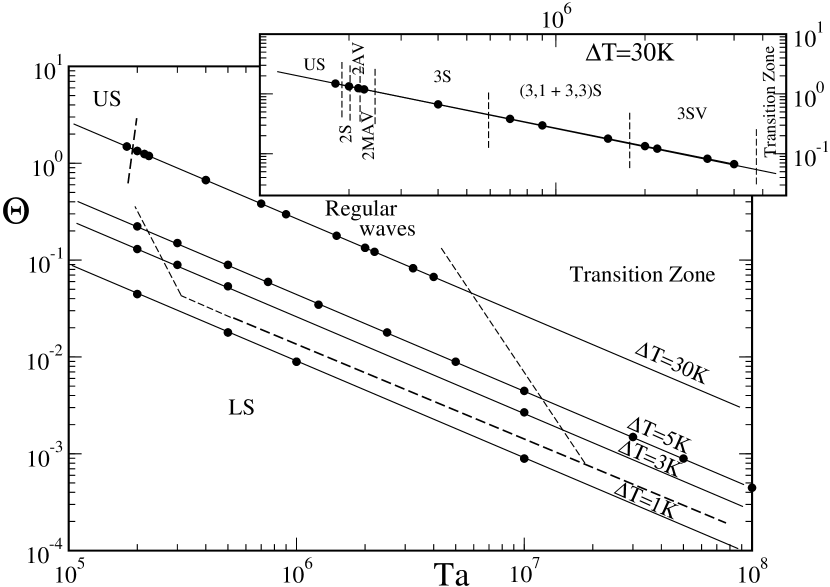
Figure 2: Summary of the regimes for air with Prandtl number of 0.7 as obtained by the numerical model. The solid lines show the temperature differences investigated in this paper and previously by [Maubert & Randriamampianina (2002)] and [Maubert & Randriamampianina (2003)]. The dots on the lines for $\Delta T=1,3,5\rm K$ correspond to cases discussed in the earlier papers while the dots on the line for $\Delta T=30\rm K$ show the cases discussed here. The dashed line indicates the transition from the symmetric regimes to regular waves, and the dotted line indicates the transition from regular waves to irregular flow. The line for $\Delta T=30\rm K$ is shown again enlarged in the insert to identify the different regimes observed in this study.

One of our objectives was to delineate a detailed regime diagram for air which was as complete as possible, similar to those already available in literature for various liquids. In Figure 2 we present a coarse-grained regime diagram obtained from direct simulation of air inside the same geometry as used by [Fowlis & Hide (1965)] in their experiments with liquids. This regime diagram uses and extends initial investigation primarily concerned with the delimitation of the axisymmetric regimes by [Maubert & Randriamampianina (2002)] and [Maubert & Randriamampianina (2003)].

The regime where all perturbations decay to an axisymmetric flow is traditionally split into a ‘Lower Symmetric’ (LS) regime, where the flow is strongly affected by viscous diffusion, and an ‘Upper Symmetric’ (US) regime, where the flow is stabilised by stratification due to the background rotation. Despite the different labels and processes involved, there exists no clear phase transition separating them. At $\Delta T=1K$, only the LS axisymmetric solution was found for all values of rotation rates considered up to a Taylor number of $Ta=10^{8}$. At higher temperature differences $3K\leq\Delta T\leq 30K$, we have delineated the transition between the symmetric regimes and regular waves. In the US regime, characterised by high values of the thermal Rossby number (and small values of the Taylor number), the heat transfer is still dominated by conduction. This transition occurs following the criterion reported by [Hide (1958)] from his experimental observations: $\Theta\leq\Theta_{crit}\equiv 1.58\pm 0.05$. Moreover, [Hide (1958)] mentioned that this anvil-like curve separating the upper symmetric regimes and the regular waves does not significantly vary with the fluid properties, say the Prandtl number $Pr$, unlike the lower symmetric transition boundary, e.g. [Fein & Pfeffer (1976)]. The computations were not extended beyond $\Delta T=30\rm K$, partly for practical reasons and partly because the validity of the Boussinesq approximation may become debatable when the volume expansion coefficient, $\Delta T/T_{0}$, becomes much larger than $0.1$. As a result, we have only confirmed the knee of the anvil in Figure 2 but not the upper, almost horizontal section of the traditional anvil.

At $\Delta T=5K$, a transition to irregular waves has been obtained through the route:
Upper symmetric flow $\rightarrow$ steady waves $\rightarrow$ quasi-periodic waves $\rightarrow$ irregular flow ([Maubert & Randriamampianina (2002)]). By convention, the term ’steady wave’ is used to identify a flow characterised by a wave of constant amplitude and drifting at a constant speed in the azimuthal direction. Substantial hysteresis was found as a result of the coexistence of different wave flow solutions under the same physical conditions, consistent with rotating experiments in liquids and many other systems of rotating flows in confined configurations. This phenomenon is also known as intransitivity. In the present case, each solution resulted from adding to the axisymmetric solution a small perturbation of a selected wavenumber to the temperature field. However, the maximum wavenumber obtained remained within the empirical limits found by [Hide (1958)]: $m_{max}\leq 0.67\pi R_{c}\approx 8$ for the present geometry. During this preliminary exploration, we did not identify clearly any vacillation regimes for $\Delta T\leq 5K$.

Some vacillation was observed at a higher temperature difference of $\Delta T=30K$ in a first exploration of this temperature contrast by [Maubert & Randriamampianina (2003)]. The work reported here continued these observations in a detailed investigation and analysis of the flow regimes obtained for this value of $\Delta T$. The specific cases discussed in detail are summarised in Table 2.

$Ta(\times 10^{5})$	$\Theta$	$\Omega$ (rad/s)	regime	$m$	$\omega_{d}$ ($2\Omega$)	$\omega_{v,m}$ ($2\Omega$)	$A_{m,1},A_{m,3}$	$\eta$
1.775	1.5087	3.617	$US$	0
1.800	1.4877	3.642	$US$	0
1.800	1.4877	3.642	$2S$	2			0.16666
1.825	1.4673	3.667	$2S$	2	0.004439		0.18335
1.850	1.4475	3.693	$2S$	2	0.003104		0.19533
2.000	1.3389	3.839	$2S$	2	0.004113		0.24676
2.050	1.3063	3.887	$2S$	2	0.006102		0.26097
2.075	1.2905	3.911	$2AV$	2	0.006647	0.05806	0.26137	0.0161
2.100	1.2752	3.934	$2AV$	2	0.00704	0.05770	0.2617	0.0343
2.150	1.2455	3.981	$2AV$	2	0.00740	0.05676	0.2630	0.0692
2.175	1.2312	4.004	$2AV$	2	0.00755	0.05630	0.2639	0.0845
2.200	1.2172	4.027	$2MAV$	2	0.00783	0.04925,	0.2684	0.1448
						0.002344
2.250	1.1902	4.072	$2MAV$	2	0.00829	0.04398,	0.2782	0.2589
						0.0037
2.2925	1.1681	4.110	$2MAV$	2	0.00893	0.04206,	0.2895	0.2993
						0.0070
2.000	1.3389	3.839	$3S$	3			0.2700
2.150	1.2455	3.981	$3S$	3			0.2991
2.250	1.1902	4.072	$3S$	3			0.3180
2.300	1.1643	4.117	$3S$	3	0.00905		0.3269
3.000	0.8926	4.702	$3S$	3	0.01551		0.3612
4.000	0.6695	5.430	$3S$	3	0.01964		0.4200
5.000	0.5356	6.070	$(3,1+3,3)S$	3	0.02094		0.4446,
							0.0721
7.000	0.3826	7.183	$(3,1+3,3)S$	3	0.02244		0.4524,
							0.1500
9.000	0.2975	8.144	$(3,1+3,3)S$	3	0.02513	0.1839	0.4469,
							0.1918
15.000	0.1785	10.514	$(3,1+3,3)S$	3	0.02732	0.1963	0.4152,
							0.2280
20.000	0.1339	12.141	$3SV$	3	0.02856	0.2183,	0.3937,	0.004131
						0.6367,	0.2297
						0.0309
22.000	0.1217	12.734	$3SV$	3	0.02857	0.1916,	0.3863,	0.009798
						0.6465,	0.2265
						0.0333
32.500	0.0824	15.477	$3SV$	3	0.02946	0.1891,	0.3598,	0.078200
						0.567,	0.2185
						0.09

Table 2: Summary of computed results for $\Delta T=30K$, with $m$ the dominant wave number.

4.2 First instability and transition to steady waves

In this section, the initial transition from the upper symmetric regime (US) to a steady wave with azimuthal wave number $m=2$ (2S), on increase of the Taylor number, will be presented. This will be followed by discussion of the subsequent transitions to an Amplitude Vacillation (2AV) and the more complex so-called ‘Modulated Amplitude Vacillation’ (2MAV; cf [Read et al. (1992)] and [Früh & Read (1997)]).

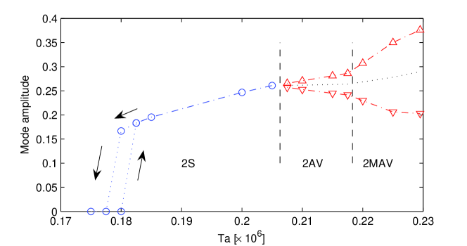
Figure 3: The amplitude of the dominant azimuthal mode, $m=2$, at mid-radius. The dash-dotted lines indicate the global maximum and minimum of the amplitude. The dash-dotted lines in the 2MAV regime denote the largest amplitude minimum and the smallest amplitude maximum of all the extreme values in each vacillation cycle, while the dotted lines in 2MAV show the average of the amplitude minimum and maximum for all vacillation cycles, respectively. The dotted line in the 2AV regime shows the averaged amplitude.

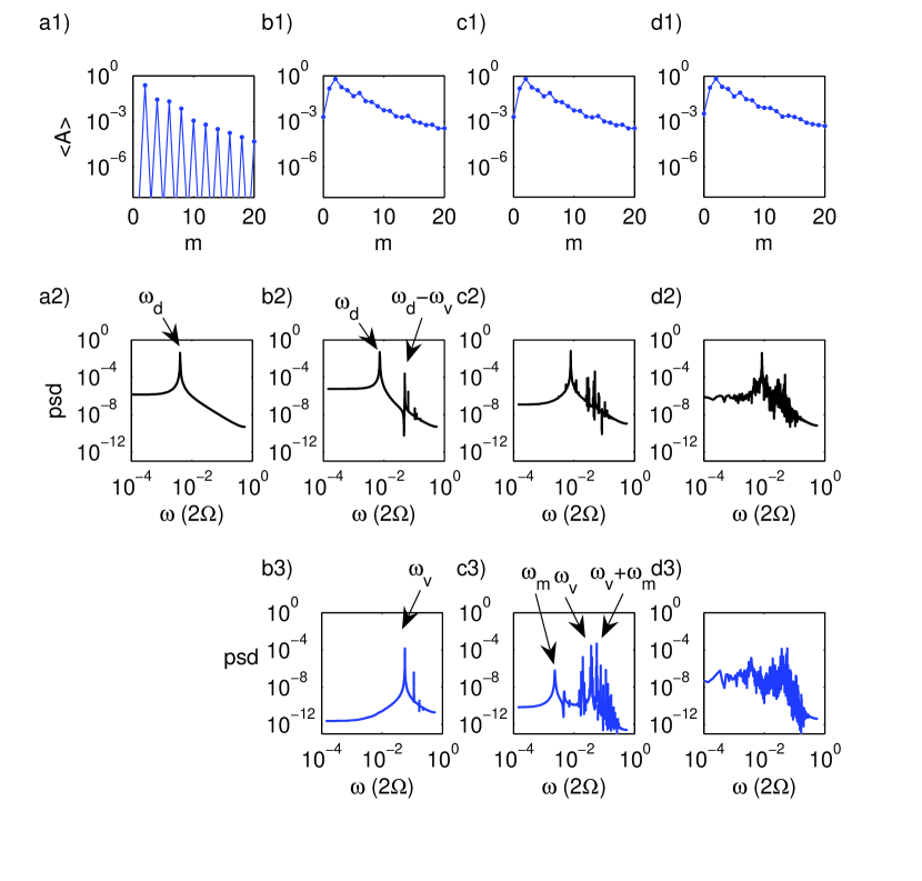
Figure 4: Spectra of representative cases of the $m=2$ flows from time series of the amplitudes of the azimuthal modes at mid-radius and mid-height. Column a) steady wave 2S, $Ta=200,000$, column b) Amplitude vacillation 2AV, $Ta=215,000$, column c) quasi-periodic modulated amplitude vacillation, 2MAV, $Ta=220,000$, and column d) irregular 2MAV, $Ta=225,000$. Top row 1): spatial spectra of the time-averaged amplitude of the azimuthal wave mode, $m$. Middle row 2) temporal spectra of the time series of the cosine component of mode $m=2$. Bottom row 3): temporal spectra of the amplitude of $m=2$. The main frequencies are indicated by their annotation, $\omega_{d}$ for the drift frequency, $\omega_{v}$ for the vacillation frequency, and $\omega_{m}$ for the modulation frequency.

The range of regimes dominated by the azimuthal wave mode $m=2$ is summarised in Figure 3, which shows the equilibrated or time-averaged amplitude of that mode. The axisymmetric baroclinic circulation was found to become unstable when the Taylor number was increased from $Ta=180,000$ to $182,500$, following which the solution converged to a steady wave mode $m=2$ and its harmonics, as a time-averaged spatial spectrum at mid-height and mid-radius demonstrates for a qualitatively similar case in Figure 4(a1). The corresponding temporal spectrum in Fig. 4(a2) of the cosine component of mode $m=2$ shows that the flow consists of a steady wave of constant amplitude travelling at a fixed angular velocity around the tank. The amplitude of the first wave solution and the step to it from the axisymmetric solution are indicated in the portion of Figure 3 indicated by ’US’ and ’2S’. The regions identified by ’2AV’ and ’2MAV’ correspond to time-dependent regimes discussed below in section 4.2.2, and the symbols represent the minima and maxima of the wave amplitude observed over time.

Decreasing the Taylor number from this first wave solution at $Ta=182,500$ back to $Ta=180,000$ did not result in a return to the axisymmetric solution but to another steady wave solution of slightly lower amplitude and higher angular velocity, as indicated in Figure 3. This hysteresis extended over a small range of Taylor number only, so that reducing the Taylor number still further to $Ta=177,000$, for example, resulted in a slow decay of the wave back to the axisymmetric solution.

4.2.1 Basic flow structures

(a)                                                                (b)

Figure 5: Horizontal cross-sections at mid-height of a 2S flow at $Ta=200,000$. (a) Temperature contours and (b) the horizontal velocity field.

An example of a typical $m=2$ flow is presented in Figures 5 to 7 of a steady wave, 2S, at a Taylor number of $Ta=200,000$. Figure 5 shows temperature contours and the horizontal velocity field at mid-level. These show the breaking of the azimuthal symmetry into a discrete symmetry of a mode with azimuthal wave number $m=2$. The velocity field can be described as a meandering jet stream, with alternating cyclones and anticyclones on either side of the jet stream. The presence of such a jet at mid-level is indicative of a significant breaking of the antisymmetry of the azimuthal flow about the mid-plane.

Figure 6: Zonal mean fields at $Ta=200,000$ using air as the working fluid. (a) Temperature (contour interval = 0.1, normalised to an imposed temperature difference of $\pm 1.0$), (b) zonal velocity $V_{\phi}$ (contour interval = 0.25) and (c) meridional stream function (contour interval = 0.01).

The basic, azimuthally-averaged flow associated with the $m=2$ waves is illustrated in Fig. 6. This shows some differences from the typical azimuthal mean state found in experiments using liquids of Prandtl number $\gg 1$. In particular, the temperature field shows relatively weakly-developed sidewall thermal boundary layers and isotherms which are steeply sloped and nearly vertical in places. On the other hand, the velocity fields and azimuthal mean stream lines such as in Fig. 6(b) and (c) indicate that Ekman layers are well developed on the rigid, horizontal boundaries while somewhat thicker, viscous Stewartson layers are present at both sidewalls.

Figure 7: Azimuth-height maps of eddy fields (with azimuthal flow removed) in a typical simulation of a 2S flow at $Ta=200,000$ using air as the working fluid. (a) Pressure (contour interval = 0.05 dimensionless units), (b) Temperature $T$ (contour interval = 0.05, normalised to an imposed temperature difference of $\pm 1.0$) and (c) Vertical velocity (contour interval = 0.1 dimensionless units).

The baroclinic character of the waves is illustrated in Fig. 7, which displays azimuth-height sections at mid-radius but with the azimuthal mean flow removed. The pressure field in Fig. 7(a) exhibits the strong ‘westward’ phase tilt with height characteristic of baroclinically unstable waves, e.g. [Hide & Mason (1975)]. The corresponding temperature field, $T^{\prime}$ in Fig. 7(b), shows a strong $m=2$ disturbance with a noticeable eastward phase tilt over most of the height range, in qualitative resemblance to the classical, linearly unstable Eady wave, e.g. [Hide & Mason (1975)]. The vertical velocity field in Fig. 7(c) is closely correlated with that of $T^{\prime}$, indicating that the fully-developed wave flow has optimised the baroclinic release of potential energy in the buoyancy field by ensuring that the upward eddy heat flux $\overline{w^{\prime}T^{\prime}}$ is as large as possible, where the $w^{\prime}$ and $T^{\prime}$ are the deviations from the temporal mean and the overbar is the time averaging of their product. The azimuthally asymmetric nature of this $m=$2S flow is again clearly apparent, but in other respects this initial instability evidently develops as a fairly ‘classical’ form of baroclinic wave with clear similarities to those found for $Pr\gg 1$ (allowing for the differing balance of diffusive effects at $Pr\sim 1$).

4.2.2 Transitions to Amplitude Vacillations

The steady wave solution remained qualitatively the same for increased Taylor number until after $Ta=205,000$, where the wave amplitude increased gradually but the angular velocity first decreased and then increased again. At $Ta=207,500$, a noticeable periodic oscillation of the amplitude was observed, exhibiting the characteristic signature of a simple Amplitude Vacillation, 2AV in this case. Figure 4 (b1) shows that the time-averaged spatial wave spectrum for the AV is fundamentally different from the steady waves, with substantial energy in wave modes other than the dominant wavenumber and its harmonics. The temporal spectra of mode $m=2$ in Figure 4 (b2 and b3) now show a second free frequency in the spectrum of the cosine component (b2) and an associated peak in the spectrum of the mode amplitude (b3). These two peaks are at different frequencies because the peak in the cosine spectrum is the difference between the vacillation and drift frequencies.

The magnitude of that vacillation is indicated by the extreme values for the wave amplitude in Figure 3 (a), where the envelope of the vacillation is shown by the maximum amplitude (the upward pointing triangles) and the minimum amplitude (the downward pointing triangles). It is quantified by the vacillation index, $\eta=(A_{max}-A_{min})/(A_{max}+A_{min})$, where $A_{max}$ and $A_{min}$ are the amplitude maximum and minimum within a vacillation cycle, respectively. This vacillation index increased first gradually then more steeply. This sharp increase in the vacillation index occurred together with the onset of a slow modulation of the vacillation, 2MAV, adding a third free frequency, as seen in Figure 4 (c3). While that spectrum is still fairly clear with sharp peaks, the spectra at $Ta=225,000$ and $229,250$ are much broader. The spatial spectra of the MAV flows as shown in Figures 4 (c1 and d1), however, are indistinguishable from that of the 2AV flow.

An important and novel point to note here is that the progression from a steady wave to an AV flow on increase of the rotation rate of Taylor number has not usually been seen in most laboratory experiments using fluids with a Prandtl number of seven and higher (e.g. [Hignett et al. (1985), Read et al. (1992), Koschmieder & White (1981)]). In their cases, the transition to AV was typically found to occur on decrease of the rotation rate (or $Ta$), where it has been observed that the transition seems to occur earlier the higher the Prandtl number ([Jonas (1981)]). An exception at high Prandtl number seems to be found close to the lower symmetric transition boundary (e.g. [Lewis & Nagata (2004)]), where the onset of AV appears via a straightforward supercritical secondary Hopf bifurcation with respect to $Ta$ or $\Theta$, much as found here for air. The present results thus indicate important roles for $Pr$ and $Ta$ in determining the nature of the bifurcation to quasi-periodic AV either as super- or sub-critical with respect to $Ta$ or $\Theta$.

4.2.3 Phase portrait analysis

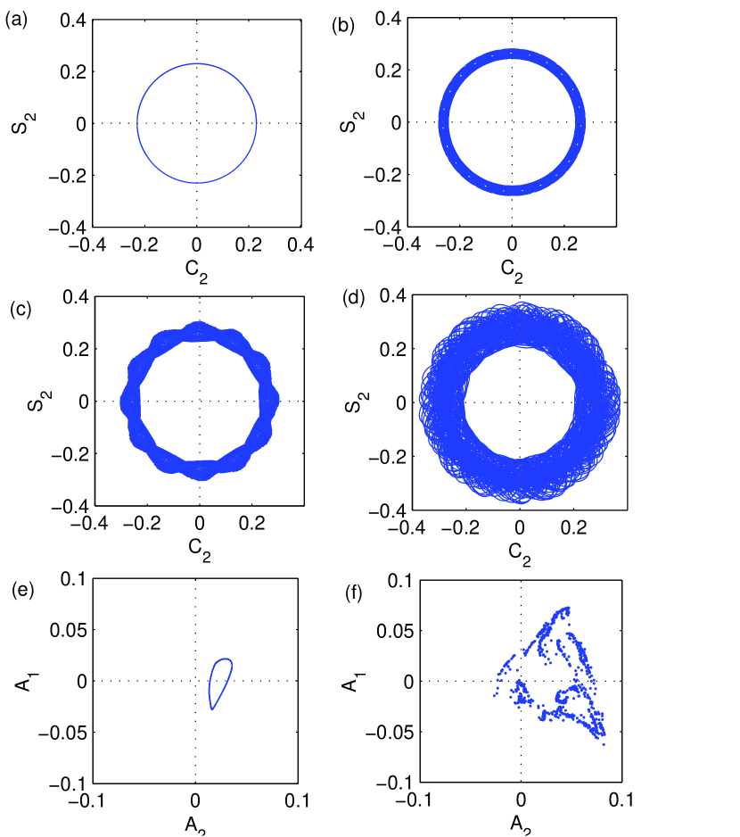
Figure 8: Phase space representations of: (a) a steady 2S (Ta= 200,000), (b) a 2AV (Ta=215,000), (c) a quasi-periodic 2MAV (Ta= 220,000), and (d) a chaotic 2MAV (Ta=229,250). The phase space diagrams show the time series of the sine component against that of the cosine component of mode $m=2$. Panels (e) and (f) show Poincaré sections of the amplitudes of $m=1$ against $m=2$ where $m=4$ is zero, after the mean amplitudes had been subtracted.

The trajectory in a reconstructed phase space or configuration space provides a way to demonstrate the different qualitative behaviours of the different flow regimes. Two representations were used here and are shown in Figure 8. One representation uses the azimuthal sine and cosine modes of a Fourier analysis of the fields at mid-height and mid-radius, the other uses the amplitude of the modes thereby removing the phase information of the wave. The trajectories, or orbits, in the projection onto the cosine and sine components of mode $m=2$ at mid-radius are shown in Figure 8 (a to d) for the different $m=2$ flows, 2S (a), 2AV (b), and two 2MAV cases (c and d). The simple circle in (a) represents the angular progression in azimuth of a wave with constant amplitude. The 2AV case in (b) shows a thickening of the circle which a Poincaré section revealed to be a torus. The large circle dominating in the phase plot in (b) still represents the drift of the wave while the small circle of the torus cross-section describes the periodic oscillation of the wave amplitude in the Amplitude Vacillation. Figure 8 (c) still shows some structure but with more detail which cannot be attributed to a simple oscillation on a torus, and (d) only retains the obvious structure of the wave mode traveling in azimuth.

If the spatial phase information is separated from the amplitude information, the amplitudes of different modes can also be used to construct an attractor of reduced dimension in a pseudo-phase space. This in effect removes the drift and its frequency from the display, the circle in Figure 8 (a) turns into a fixed point, the torus in (b) into a limit cycle, and a 3-torus into 2-torus. To analyse the 2MAV flow, a Poincaré section of the amplitude trajectory is required. A section to the 2MAV case at $Ta=220,000$ in Figure 8(e) reveals that the orbit in the amplitude space is a 2-torus, and therefore that the 2MAV shown in (c) is a 3-torus. This implies that this particular 2MAV flow is a quasi-periodic flow with three independent and incommensurate frequencies. This is a remarkable case since [Newhouse et al. (1978)] have argued that generic 3-frequency flows are usually unstable.

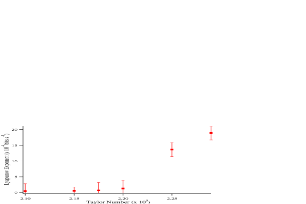
Figure 9: The largest Lyapunov exponent for the 2AV and 2MAV flows against Taylor number.

The Poincaré section for the other 2MAV cases at $Ta\geq 225,000$ appear to be more typical of chaotic flows as illustrated by Figure 8 (f) for $Ta=229,250$. Figure 8 (f) only shows the positive crossings for reason of clarity but the crossings in the negative direction are qualitatively the same and are found in a region which overlaps with that occupied by the positive crossings. This is in contrast to the quasi-periodic 2MAV where the crossing the different directions occupy distinct and well-separated regions. As a test for low-dimensional chaotic behaviour, the largest Lyapunov exponent, $\lambda_{1}$, was calculated for all the AV and MAV cases, using the method of [Wolf et al. (1985)]. As Figure 9 shows, the flows at low Taylor number up to, and including, the 2MAV case at $Ta=220,000$ have a largest Lyapunov exponent which cannot be distinguished from zero. However, $\lambda_{1}$ is significantly positive for the last two 2MAV cases. A positive Lyapunov exponent is clear evidence for chaotic solutions, indicating that a clear transition to low-dimensional chaotic behaviour occurs, but only after the quasi-periodic transition to 2MAV. The intermediate 2MAV case has a value for $\lambda_{1}$ which is indistinguishable from zero, confirming the existence (hinted at above) of a nonchaotic three-frequency flow.

4.3 Transition to $m=3$ and higher modes

As $Ta$ was increased through the 2MAV regime discussed above, the flow dominated by $m=2$ was found to give way to a new type of flow dominated by $m=3$ at $Ta=2.3\times 10^{5}$. We consider in this subsection the flow structure and transitions from the $m=3$ state as Taylor number is varied.

4.3.1 Basic flow structures

(a)                                                                (b)

Figure 10: Horizontal cross-sections at mid-height of a wave-3 flow at $Ta=1.5\times 10^{6}$. (a) Temperature contours and (b) the horizontal velocity field.

The basic flow pattern is illustrated in Figures 10 to 12 for a steady wave, 3S, at $Ta=1.5\times 10^{6}$. Figure 10 shows maps in the $(r,\theta)$ plane of temperature and velocity vectors at mid-height for a typical $m=3$ case. The temperature fields show the presence of pronounced ‘plumes’ alternately of warm and cool air, highly concentrated in azimuth and crossing the annular gap radially in association with strong radial jets.

Figure 11: Azimuth-height maps of eddy fields (with azimuthal flow removed) in a typical simulation of the wave-3 flow at $Ta=1.5\times 10^{6}$ using air as the working fluid. (a) Pressure (contour interval = 0.25 dimensionless units), (b) Temperature $T$ (contour interval = 0.05, normalised to an imposed temperature difference of $\pm 1.0$) and (c) Vertical velocity (contour interval = 0.5 dimensionless units).

The barotropic nature of the fully developed waves in this region of parameter space is illustrated in Fig. 11, which shows azimuth-height sections of an $m=3$ flow at $Ta=1.5\times 10^{6}$. The pressure field (Fig. 11(a)) clearly shows very little phase tilt with height, in complete contrast to those in the 2AV regime shown in Figure 7. The temperature field in Figure 11(b), too, has a much more complicated structure than for the $m=2$ flows, with highly concentrated plumes of hot and cold air which have very little slope with height, interspersed with broad regions with relatively very weak horizontal thermal gradients. The thermal plumes are aligned azimuthally with the regions of strong azimuthal pressure gradient, consistent with optimising the correlation between radial (geostrophic) velocity and temperature perturbations. Similarly, the regions of strong upward vertical velocity (Fig. 11(c)) are also concentrated close to the strongest positive temperature anomalies, and vice versa, consistent with an optimisation of $\overline{w^{\prime}T^{\prime}}$ as before. Regions of strong downward motion (necessary to satisfy mass conservation) are concentrated in plumes or jets adjacent to the strong upwelling jets, forming ‘cross-frontal’ circulations which show some similarities with those inferred for atmospheric frontal regions in developing cyclones ([Hoskins (1982)]). The overall impression is that the flow in this region of parameter space is strongly nonlinear and much modified from the simple, linearly unstable Eady solution of the corresponding state for $m=2$ flows at much lower Taylor number.

Figure 12: Zonal mean fields for the typical wave-3 simulation at $Ta=1.5\times 10^{6}$ using air as the working fluid. (a) Temperature (contour interval = 0.1, normalised to an imposed temperature difference of $\pm 1.0$), (b) zonal velocity $V_{\phi}$ (contour interval = 0.25 dimensionless units) and (c) meridional stream function (contour interval = 0.01 dimensionless units).

The increasingly barotropic and nonlinear character of the flow at high $Ta$ is also apparent in the azimuthal mean flow structure, which is illustrated in Fig. 12. This time, in contrast to the low $Ta$ states (fig. 6), the temperature field (Fig. 12(a)) exhibits strongly developed sidewall thermal boundary layers and relatively weak horizontal thermal gradients in the interior. The near-absence of horizontal thermal contrast in the interior would suggest (via the geostrophic thermal wind relation) that the zonal flow should be relatively barotropic. This is confirmed in Fig. 12(b), which shows negative (retrograde) azimuthal flow at most heights except near the outer cylinder. The zonal mean meridional streamlines (Fig. 12 (c)) exhibit an additional (thermally indirect) ’Ferrel’ cell, in contrast to Fig. 6 (c), indicating a strong contribution of baroclinic eddies to the heat transport in this case.

4.3.2 Sequence of flow transitions

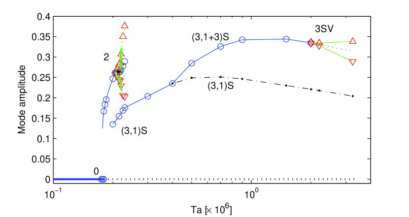
Figure 13: The amplitude of the $m=3$ solutions against the Taylor number. The solid line and circles show the sum of the first three radial modes of the azimuthal mode $m=3$, while the dash-dotted line only shows the contribution of the first radial mode. For the vacillating flows, the mean amplitude is given by the dotted lines, and the amplitude extrema are shown by the solid lines and triangles. To put the $m=3$ solutions into context, the transition from axisymmetric flow and the $m=2$ solutions, shown in Figure 3 are reproduced.

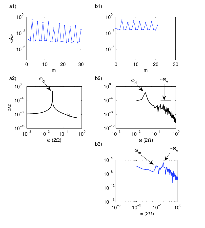
Figure 14: Spectra of representative cases of the $m=3$ flows from time series of the amplitudes of the azimuthal modes at mid-radius and mid-height. Column a) steady wave 3S, at $Ta=0.9\times 10^{6}$, and column b) irregular structural vacillation, 3SV, at $Ta=3.25\times 10^{6}$. Top row 1): spatial spectra of the time-averaged amplitude of the azimuthal wave mode, $m$. Middle row 2): temporal spectra of the time series of the cosine component of mode $m=3$; Bottom row 3): temporal spectra of the amplitude of $m=3$. The main frequencies are indicated by their annotation.

The onset of $m=3$ effectively began a new sequence of bifurcations, since the $m=3$ flow at $Ta=230,000$ converged to a regular pattern of a steady amplitude of $m=3$ and its harmonics, as shown by the time averaged amplitude spectra in row 1 of Figure 14. The new solution showed substantial hysteresis relative to the previous $m=2$ regime in that reducing the Taylor number to $Ta=200,000$ still gave a steady $m=3$ solution. This 3S regime persisted until $Ta=1.5\times 10^{6}$ but at $Ta=2\times 10^{6}$ other frequencies emerged. The sequence of $m=3$ flows observed can be illustrated by Figure 13 which shows the amplitude of the azimuthal mode $m=3$, where the solution branch of the $m=2$ flows (Fig. 3) is reproduced to put the $m=3$ observation in context.

The sum of all radial modes of the azimuthal mode at mid-radius resulted in an initial increase of the amplitude on increase of the Taylor number followed by a decrease, which was mirrored by a continuing increase of the amplitude at a radius of one quarter of the gap from the inner wall three quarters. This suggested that the radial structure of the flow was more complex. Approximating the radial structure by half sine waves, the approximate distribution into the first three radial modes, $A_{m,n}$ with $m=3$ and $n=1,2,3$, can be estimated from the amplitudes, $A_{1/4},A_{1/2},A_{3/4}$ at a radial position of a quarter, a half, and three-quarters of the gap, respectively, by

$$n=1 : A_{3,1}=\frac{1}{\sqrt{8}}\left(A_{1/4}+A_{3/4}\right)+\frac{1}{2}A_{1/2}$$

$$n=2 : A_{3,2}=\frac{1}{2}\left(A_{1/4}-A_{3/4}\right)$$

$$n=3 : A_{3,3}=\frac{1}{\sqrt{8}}\left(A_{1/4}+A_{3/4}\right)-\frac{1}{2}A_{1/2}.$$

Figure 13 then shows the amplitude of the sum of first three radial modes as the solid line, labeled with ’(3,1+3)S’ since the second radial mode did not contain any substantial amplitude. Below $Ta\approx 400,000$, the overall amplitude is fully described by the first radial mode only. Following this branch to lower values of the Taylor number, one can observe a substantial regions of hysteresis between the $m=2$ branch and the $m=3$ branch. Between $Ta=400,000$ and $Ta=500,000$, the radial structure of the flow changes whereby $(m=3,n=3)$ grows beside $(m=3,n=1)$. In terms of the horizontal structure of the flow, this indicates the emergence of a flow with wave trains near either side wall. Finally, this solution develops a vacillation which appears as a radial fluctuation of the eddies or wave maxima. Visually, this vacillation would be classified as a structural vacillation since the overall amplitude (still dominated by the first radial mode) varies little, but the exchange between flow or temperature maxima at mid-radius and near the walls varies the structure of the flow.

4.3.3 Spatial and temporal spectra

Figure 14 shows a set of time-averaged mode spectra in row (1) and corresponding power spectra for the cosine component of $m=3$ (row 2) and for the amplitude of $m=3$ in row (3). A steady wave case and a vacillating case are shown. While the transition from 2S to 2AV discussed above was characterised by a fundamental change in the time-averaged spectrum, the mode spectra for all wave-3 flows are qualitatively very similar. The only substantial change is the gradual increase of the ’floor’ from around $10^{-5}$ to around $10^{-3}$.

Because the vacillation of the amplitude is very weak in almost all cases, the power spectrum of the cosine component of $m=3$, the upper of the spectral curves in each plot in row 2 of Figure 14, is very bland and only shows the distinctly the peak at the drift frequency of the wave. The power spectrum of the amplitude, however, shows two broad but distinct peaks, one associated with vacillation of the flow structure and the other with a slower modulation. We did not observe any periodic vacillation in this set of simulations. It should be noted, however, that the transients leading to the steady 3S solutions were characterised by a decaying, periodic oscillation with oscillation frequencies comparable to the vacillation frequency identified in Figure 14 (b3).

4.3.4 Phase portraits

(a)                                                               (b)

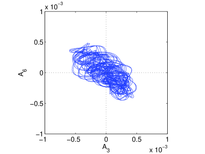
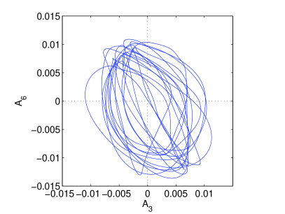
(c)                                                    (d)

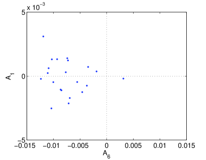
Figure 15: Phase portraits and Poincaré sections in the $m=3$ regime: (a) Phase portrait of the amplitude of $A_{6}$ against $A_{3}$ for $Ta=2.0\times 10^{6}$, (b) Phase portrait for $Ta=3.25\times 10^{6}$; (c) Poincaré section at $A_{3}=0$ showing $A_{1}$ against $A_{6}$ for $Ta=2.0\times 10^{6}$. (d) Poincaré section as (c) but for $Ta=3.25\times 10^{6}$.

Figure 15 shows phase portraits and Poincaré sections of two vacillating cases, the first time-dependent case at $Ta=2\times 10^{6}$ and the final case at $Ta=3.25\times 10^{6}$. Since the strength of the vacillation is very small compared to the mean amplitude, only the phase portraits generated from the wave amplitudes are shown; the phase portraits for the cosine or sine components would only show the circle representing the wave drift. Both cases show irregular oscillations of the amplitude in the phase portrait of the amplitude of mode $m=6$ against that of $m=3$. The Poincaré section of the phase portrait for the lower Taylor number in Figure 15 (c), which shows the amplitude of $m=1$ against that of $m=6$ at the section where $A_{3}=0$ reveals no obvious structure at all. The corresponding section for the high Taylor number is also irregular but it appears that at least the negative crossing points are arranged around a circular structure indicating the possibility of a fuzzy torus. It has to be noted that the scale of the plots varies substantially between the two cases with the $y$-axis 5 times larger and the $x$-axis 50 times larger in Figure 15 (d) compared to Figure 15 (c). Due to the computational expense of the calculations at these high Taylor numbers, the time series at the highest value of Ta, only covers a few drift periods of the dominant flow feature which is too short to estimate Lyapunov exponents. For the same reason, it has not been possible to carry out more integrations between $Ta=2.2\times 10^{6}$, which is qualitatively and quantitatively similar to $Ta=2.0\times 10^{6}$, and $Ta=3.25\times 10^{6}$ to investigate whether the toroidal structure seen in Figure 15 (d) is a larger-amplitude version of the fluctuations seen in Figure 15 (c) or whether it emerges as a new type of oscillation besides the small-scale fluctuations in a flow regime transition. As a final note it should be mentioned that no quasi-periodic solutions were found in the simulations carried out.

5 Discussion

5.1 Regime diagram and onset of baroclinic waves

The overall structure of the regime diagram, presented in Figure 2, is qualitatively and quantitatively consistent with previous experiments and simulations of the baroclinic annulus using liquids instead of air. They all show the characteristic anvil shaped transition curve between axisymmetric flow and regular waves, separating the regimes into a wave regime, an upper symmetric regime at large $\Theta$, and a lower symmetric regime at small $\Theta$/small Taylor number, e.g. [Fein (1973), Fein & Pfeffer (1976), Hide (1958), Hide & Mason (1975)] and [Jonas (1981)]. The upper symmetric regime indicates a flow at large $\Theta$ or thermal Rossby number which is stabilised by strong stratification. The transition from the upper symmetric regime to baroclinic waves appears largely controlled by a critical thermal Rossby number. The lower symmetric regime is stabilised by viscous dissipation, and the transition to waves is largely given by a critical Grashof number or Rayleigh number.

Most of these had been performed with fluids of Prandtl number $Pr>\sim 7$ but even an early study by [Fein & Pfeffer (1976)] using mercury, with $Pr=0.025$, showed the same qualitative characteristic anvil shaped stability curve although the onset of waves was shifted towards higher Taylor numbers by several orders of magnitude. The case of air with a Prandtl number between that of mercury and water, however, seemed not to be located between those cases but, if anything, at slightly small values of the Taylor number. The observations from our simulations suggest that the case of $\Delta T=30K$ is positioned near the ’knee’ of the classical anvil shape.

The, albeit narrow, hysteresis at the transition between the axisymmetric flow and the steady wave suggests a subcritical bifurcation. While [Hide & Mason (1978)] reported that the transition from the symmetric regimes in an annulus showed hysteresis only if the upper boundary was a free surface, [Koschmieder & White (1981)] presented evidence for the possibility of small hysteresis for the transition to or from the upper symmetric regime. In their experiments, performed with water ($Pr\sim 7$), the hysteresis set in at a critical Taylor number below which the transition was not hysteretic and above which the extent of the overlap of the symmetric and wave regimes increased with the Taylor number. Hysteresis near the ’knee’ of the anvil-shaped marginal stability curve has not been documented before. Other studies have either reported or assumed a Hopf bifurcation, e.g. [Rand (1982), Miller & Butler (1991), Lewis & Nagata (2004)], or the occurrence of so-called weak waves prior to the onset of fully-developed baroclinic waves, [Hide & Mason (1978), Jonas (1980)]. The weak waves have been suggested to be wave modes which are located near the upper or lower boundary and are decaying in the fluid interior. No such weak waves were observed in this study, though it has to be said that weak waves seem to have been observed predominantly at the transition from the upper symmetric regime at somewhat higher Taylor numbers, well past the knee of the anvil.

5.2 A bifurcation scenario

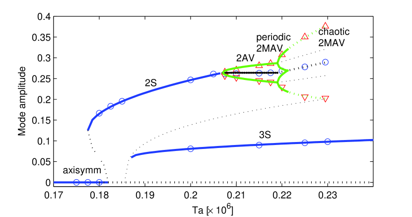
Figure 16: The bifurcation scenario for the transition from the upper symmetric regime to a steady wave and subsequent vacillations for the $m=2$ flows.

The transition sequence from the axisymmetric flow through all observed wave 2 flows follows clear steps of increasing complexity, from axisymmetric flow via a steady wave with one frequency, a two-frequency flow of a vacillating wave, a quasi-periodic three-frequency flow of a modulated vacillating wave to, finally, a chaotic flow. As Hopf bifurcations for the onset of baroclinic waves and the subsequent onset of amplitude vacillation are often cited, e.g. [Rand (1982), Miller & Butler (1991), Lewis & Nagata (2004)], it seemed obvious to fit the normal form of a Hopf bifurcation to the wave amplitude data. This transition scenario is reproduced in Figure 16 by showing the mean amplitude and the envelope of the vacillation.

Since the initial onset of waves is a subcritical transition, a subcritical Hopf bifurcation and a Fold or saddle-node bifurcation is invoked, e.g. [Guckenheimer & Holmes (1983), Rand (1982)]. A linear regression to a curve of the form $A=A_{0}+[(Ta-Ta_{S})/q]^{1/2}$, using the five data points from the 2S regime, gave $A_{0}=0.125$ for the wave amplitude at the saddle-node, a growth parameter of $q=1.50\times 10^{6}$, and a critical Taylor number for the saddle-node of $Ta_{S}=177,500$ with a correlation coefficient of $r^{2}=0.9997$. The ’unstable branch’ has been filled in using this critical Taylor number and a Taylor number for the location of the unstable Hopf as $Ta_{0}=182,000$.

The following transition, from the steady wave to the periodic oscillation of the wave amplitude in the 2AV flow, is consistent with a second Hopf, also known as a Neimark bifurcation. This is indicated by fitting a square-root function to the vacillation strength (amplitude maximum minus mean amplitude) for the four simulations in the 2AV regime as a function of the Taylor number. While this is a standard bifurcation, it is in contrast to all experience for the onset of amplitude vacillation in a liquid with a range of Prandtl number between 7 and 30, where the evidence is that vacillation occurs on decreasing the Taylor number from the steady wave. In those cases, the vacillation is a precursor to a particular wave mode giving way to, and co-existing with, a flow of lower mode number. The experiments in mercury by Fein and Pfeffer from 1976 at much lower Prandtl number did not report such details in the wave regime. The consensus for the other experiments in liquids is that vacillation is much more common in higher Prandtl number, where most of the wave 2 and 3 domains at $Pr=26$ in [Früh & Read (1997)] were time-dependent, whereas at $Pr=13$ and $Pr=7$ substantial ranges were found where a steady wave was reported by [Hignett (1985), Hignett et al. (1985), James et al. (1981)]. Some initial experiments carried out in the apparatus used by [Hide & Mason (1978), Read et al. (1992), Früh & Read (1997)] but now using air confirmed at least qualitatively the onset of vacillation with increasing Taylor number, consistent with these computational results.

The third transition, to a modulated 2MAV was a not surprising continuation of the ’quasi-periodic route to chaos’ described by [Newhouse et al. (1978)], see also §6 in [Schuster (1995)], but the nature of the initial solution as a quasi-periodic 2MAV with three independent frequencies was unusual. As was shown by [Newhouse et al. (1978)], generic three-frequency flows are expected to be chaotic rather than periodic. Previous illustrations of the existence of three-frequency quasi-periodic orbits were demonstrated numerically, with the modulation of a simple circle map by [Grebogi et al. (1983b)], and in experiments of convection of mercury in a magnetic field by [Libchaber et al. (1983)]. However, no previous example such a flow has been reported from either numerical or experimental studies of baroclinic waves. All previous reports of quasi-periodic modulated vacillations, e.g. by [Read et al. (1992)] and [Früh & Read (1997)], involved frequency-locking between the drift frequency and the vacillation or modulation frequency. Conversely, no instance of frequency-locking was observed in the current numerical simulations. This supports the previously suggested notion that the ubiquitous frequency locking in the baroclinic annulus relies on a coupling between the spatial phase of the wave and its amplitude by imperfections in the apparatus or the presence of sensors in the fluid.

The final type of flow dominated by $m=2$ was a chaotic 2MAV. In the average statistics, such as the time-averaged wave spectrum and the average drift frequencies, there was little difference between the quasi-periodic and the chaotic versions of the 2MAV. Fitting yet another square-root function to the modulation amplitude over the vacillation amplitude in the MAV regimes suggests that the onset of modulation in itself could be consistent with a further supercritical Hopf bifurcation. As there are only three sufficient 2MAV simulations, together with a change in character from quasi-periodic to chaotic, the assumption of a square-root scaling is conjecture but gives a reasonable representation of the development of the modulation. Square-root dependent or not, the growth of the modulation hints at the possible mechanism for the transition from periodic to chaotic behaviour: the minimum of the amplitude maximum and the maximum of the amplitude minimum intersect in Figure 16 at a point between the observed periodic flow at $Ta=220,000$ and the first chaotic flow at $Ta=225,000$. It appears therefore, that the transition to chaos in this example might not have arisen from the local stretching of the torus, §6.1 in [Schuster (1995)], but from a crisis as suggested by  [Grebogi et al. (1983b)] where the orbit of the quasi-periodic 2MAV intersects the unstable orbit of the 2AV, see also §6.4 in [Schuster (1995)].

The final transition from the $m=2$ branch to the steady 3S on the $m=3$ solution branch could also be due to a crisis, this time caused by the collision of the chaotic 2MAV attractor with the unstable orbit separating the $m=2$ and $m=3$ solutions. Such a collision is possible in phase space because the 2MAV flow involves finite-amplitude variations of the $m=3$ mode, and it is consistent with the conjecture by [Grebogi et al. (1983b)] that ’almost all’ sudden changes in chaotic attractors are due to crises. The existence of an unstable orbit separating the basin of attraction of the $m=2$ and $m=3$ solutions is indicated by the dotted line between the two solution branches, following Figure 8 of [Lewis & Nagata (2003)].

5.3 Transitions on the $m=3$ branch

The $m=3$ flows also showed a progression from periodic flow of a steady wave, 3S, to irregular vacillations but following a very different route. This route involved a change in the radial structure of the flow while remaining a simply-periodic flow of a steady wave. No quasi-periodic flows were observed but the possibility remains that those could exist at Taylor numbers not covered by the simulations.

The vacillating flows at the very high Taylor number are qualitatively similar to experimental evidence by [Früh & Read (1997)] at $Pr=26$ which they classified as ’Structural Vacillation’, also known as ’Tilted-trough vacillation’. That flow was largely dominated by a simple azimuthal mode ($m=2$ in their case), superimposed on which were small fluctuations consistent with a higher radial mode. While the large scale structure of the flow was highly regular, the fluctuations were shown by them to be not consistent with low-dimensional dynamics. The failure to compute reliable dimension estimators for structural vacillation had previously been reported in two independent experimental studies by [Read et al. (1992)] and [Guckenheimer & Buzyna (1983)].

The significantly different vertical structure of the steady 3S, by being much more barotropic, could result in a different type of instability altogether. The radial profile of the azimuthal velocity, shown in Figure 12 (b) suggests a Reynolds number of $Re\equiv UL/\nu\approx 50$ for the boundary layer near the inner wall (using a velocity of $\sim 12U$ at a distance of $L\sim 0.1b$ from the wall). Studies of the instability of detached shear layers by [Früh & Read (1999)] suggest that such a Reynolds number is sufficient for the onset of barotropic instability in a Hopf bifurcation which leads to a string of vortices along the shear layer with a wave number largely determined by the thickness of that layer. With a critical Taylor number of $Ta_{c}=428,000$, the observed growth of the higher radial mode, shown in Figure 13, is consistent with a square-root dependence up to the Taylor number of $Ta=900,000$. Barotropic instability has also been proposed by [Schär & Davies (1990)] as a mechanism active in the decay of baroclinic waves in the atmosphere. If this instability has caused the onset of the waves near the side walls, it is not surprising that the quasi-periodic route to chaos was not followed, as the experiments by [Früh & Read (1999)] did not observe quasi-periodic vacillating flows either. The indication of steps of a period-doubling cascade were observed at large Rossby numbers, whereas the increase in Taylor number in the baroclinic annulus would result in reducing the Ekman number in their study. At a Reynolds $Re=O(50)$, they observed only steady and noise waves of wave number $m\geq 6$ and a regime of weak irregular fluctuations (cf their regime diagram in the $Re-E$ plane in Figures 3 in [Früh & Nielsen (2003)]). [Früh & Nielsen (2003)] suggested that the onset of time-dependence in the amplitude of barotropic vortices may rely on local, small-scale vorticity generation at the side walls rather than a global-mode instability of the flow in the fluid interior.

6 Conclusions

	US		axisymmetric
Subcritical Hopf	$\leftarrow|\rightarrow$	2S	baroclinic instability,
with saddle-node			zonal symmetry breaking
Hopf	$\longleftrightarrow$	2AV	temporal symmetry breaking
Hopf	$\longleftrightarrow$	2MAV	three-frequency quasi-periodic
Crisis	$\longleftrightarrow$	2MAV	chaos
Crisis	$\leftarrow|\rightarrow$	3S	mode transition,
			zonal symmetry breaking
Pitchfork	$\longleftrightarrow$	(3,1 + 3,3)S	barotropic instability,
			radial symmetry breaking
???	$\longleftrightarrow$	3SV	irregular fluctuations

Table 3: Tentatively suggested bifurcation sequences from the initial instability to the onset of the irregular vacillation of the $m=3$ flow. $\longleftrightarrow$ denote transitions without hysteresis (supercritical bifurcations), and $\leftarrow|\rightarrow$ indicate the presence of hysteresis.

We have presented results from direct numerical simulations of convection in a baroclinic annulus filled with air and put those in the context of sloping convection in liquid-filled baroclinic annulus experiments. This investigation, and the two previous studies by Maubert & Randriamampianina (2002,2003) leading up to this work, followed the most common procedure of keeping the temperature difference fixed while varying the rotation rate of the system. Maubert & Randriamampianina (2002,2003) verified the transition curve between the symmetric regimes and wave regimes and they reported the main types of baroclinic waves usually observed in the baroclinic annulus. The transition curve from the axisymmetric solution to steady, fully-developed baroclinic waves formed the typical anvil shape in the $Ta-\Theta$ parameter plane, in common with all published information on this transition for liquids covering a range of Prandtl number from 0.025 to 26 (though not the extreme case published by [Fein & Pfeffer (1976)] for $Pr=63$).

Table 3 summarises the sequence of flows and bifurcations. The initial baroclinic instability and the development of the $m=2$ flows are consistent with the standard quasi-periodic route to chaos with a few individual aspects, such as the subcritical character of the first Hopf bifurcation and the existence of a rather rare three-frequency quasi-periodic flow which became chaotic in what could be a crisis. The mode transition between flows dominated by $m=2$ and $m=3$, respectively, is also consistent with all previous evidence for baroclinic waves in the rotating annulus in that it is a sudden mode transition to a higher wave number on increase of the Taylor number, associated with a substantial hysteresis.

The results at the highest Taylor number achieved in the study points to a first direct numerical simulation of a structural vacillation. The onset and characteristics of structural vacillation is less well documented in the literature, where a variety of small-scale processes have been proposed, e.g. [Früh & Read (1997)], such as inertia-gravity waves observed by [Lovegrove et al. (2000)]. The evidence here points to the occurrence of a barotropic instability of the steady wave prior to the onset of temporal fluctuations near the side walls, in which case vorticity generation at the side walls may be a mechanism in the onset of structural vacillation in the annulus.

Overall, the observations are consistent with the extensive literature on baroclinic waves in the thermally forced annulus filled with liquids. This demonstrates the validity of the numerical model in parameter ranges not previously covered by direct numerical simulation. The change in Prandtl number from $Pr\gg 1$ to $Pr<\sim 1$, however, resulted in the reversal of the Hopf bifurcation leading to amplitude vacillation. From a physical point of view it seems sensible to suggest that the relative thickness of the thermal and velocity boundary layers controls whether the vacillation appears on increase or decrease of the Taylor number. While this change in itself is rather subtle, it has consequences for the overall organisation of the regime diagram and the transition from highly regular to complex flows. This point is not only relevant to baroclinic annulus flows but to all convective flows, if not fluid dynamical systems in general, where a change in the fluid properties may lead to apparently minor changes which then cause a fundamental change in the dynamics over a wide range of forcing parameters.